Using Swarm to Detect Total Water Storage Changes in 26 Global Basins (Taking the Amazon Basin, Volga Basin and Zambezi Basin as Examples)

Abstract

The Gravity Recovery and Climate Experiment (GRACE) satellite provides time-varying gravity field models that can detect total water storage change (TWSC) from April 2002 to June 2017, and its second-generation satellite, GRACE Follow-On (GRACE-FO), provides models from June 2018, so there is a one year gap. Swarm satellites are equipped with Global Positioning System (GPS) receivers, which can be used to recover the Earth’s time-varying gravitational field. Swarm’s time-varying gravitational field models (from December 2013 to June 2018) were solved by the International Combination Service for Time-variable Gravity Field Solutions (COST-G) and the Astronomical Institute of the Czech Academy of Sciences (ASI). On a timely scale, Swarm has the potential to fill the gap between the two generations of GRACE satellites. In this paper, using 26 global watersheds as the study area, first, we explored the optimal data processing strategy for Swarm and then obtained the Swarm-TWSC of each watershed based on the optimal results. Second, we evaluated Swarm’s accuracy in detecting regional water storage variations, analyzed the reasons for its superior and inferior performance in different regions, and systematically explored its potential in detecting terrestrial water storage changes in land areas. Finally, we constructed the time series of terrestrial water storage changes from 2002 to 2019 by combining GRACE, Swarm, and GRACE-FO for the Amazon, Volga, and Zambezi Basins. The results show that the optimal data processing strategy of Swarm is different from that of GRACE. The optimal results of Swarm-TWSC were explored in 26 watersheds worldwide; its accuracy is related to the area size, runoff volume, total annual mass change, and instantaneous mass change of the watershed itself, among which the latter is the main factor affecting Swarm-TWSC. Knowledge of the Swarm-TWSC of 26 basins constructed in this paper is important to study long-term water storage changes in basins.

1. Introduction

The Gravity Recovery and Climate Experiment (GRACE) satellite is the first satellite mission dedicated to Earth gravity sounding, launched by the National Aeronautics and Space Administration (NASA) and the German Aerospace Center (DLR). In the decade since its launch in March 2002, GRACE has been widely used to detect Earth-mass transport, including total water storage change (TWSC) [1,2], changes in the Antarctic and Greenland ice caps [3,4], and global sea-level changes [5,6], making important contributions to Earth science-related research and functioning as an important tool for estimating changes in terrestrial water reserves. However, in September 2017, one of the batteries in the GRACE-2 satellite failed, and its mission was successfully ended in mid-October 2017 [7,8]. Now, the GRACE time-varying gravity field model provided by the three major international centers, the Jet Propulsion Laboratory (JPL), the University of Texas Space Research Institute (CSR), and the German Geosciences Research Center (GFZ), is currently up to date only as of June 2017. The successor to the GRACE mission, GRACE Follow-On (GRACE-FO), was successfully launched on 22 May 2018 in California, USA, and its measurement principle is similar to that of GRACE, so its model can be used to continue the study of TWSC. However, the GRACE-FO time-varying gravity field model data are now published from June 2018, which means that there is a one-year gap between GRACE and GRACE-FO, so, valid and reliable data need to be found to fill this gap and ensure the consistency of the time-varying gravity field information time series.

On 22 November 2013, the European Space Agency (ESA) successfully launched an Earth observation satellite constellation, Swarm, consisting of three satellites, similar to the Challenging Mini-satellite Payload (CHAMP) mission. Although its mission is mainly to monitor the Earth’s magnetic field variations, it can also be applied to study the time-varying gravity field because it carries high-precision Global Navigation Satellite System (GNSS) receivers and other key gravity detection equipment, thus filling the observation gap between GRACE and GRACE-FO [9]. The published Swarm time-varying gravity field models are the model from December 2013 to June 2019, solved by COST-G, and the model from December 2013 to October 2018, solved by ASI. The Swarm of both institutions allows the continuity of GRACE and GRACE-FO observations on a time scale, so it is particularly important to determine the feasibility and effectiveness of the Swarm-based model to recover changes in terrestrial water storage. In recent years, several scholars have used the Swarm time-varying gravity field model to detect water storage changes in basins. Lück et al. (2018) studied the possibility of Swarm bridging GRACE and GRACE-FO, and the possibility of using Swarm time-varying gravity field with significantly lower resolution to replace GRACE time-varying gravity field in missing months [10]. Meyer et al. (2019) provided a long-term time series of monthly gravity field solutions by combining laser satellite data, GPS and K/Ka band observations of GRACE mission and GPS observations of three Swarm satellites. In their study, the lunar gravity field from Swarm was used to fill the gap between GRACE and GRACE-FO tasks [11]. Li et al. (2019) used the Swarm time-varying gravity field to estimate terrestrial water storage changes in the Amazon Basin and the water storage deficit caused by the 2015/2016 drought event. Comparing GRACE data, hydrological models, and hydrological station data, they found that the Swarm results were in good agreement with GRACE, hydrological models, and virtual hydrological station estimates, providing a new and effective way to detect terrestrial water storage changes and drought events. It also has the potential to replace the GRACE satellite to detect extreme droughts and floods in the Amazon basin [12]. Cui et al. (2020) compared Swarm with the GRACE/GRACE-FO models in terms of model accuracy, observation noise, and inverted TWSC and the results verified that Swarm time-variable gravity field has the potential to extract TWSC signals in the Amazon River Basin and can serve as a complement to GRACE/GRACE-FO data for detecting TWSC in local areas [13]. Forootan et al. (2020) applied time-variable gravity fields (2013 onward) from the Swarm Earth explorer mission with a low spatial resolution of ∼1500 km. A novel iterative reconstruction approach was formulated based on independent component analysis (ICA) combining GRACE and Swarm fields. The reconstructed TWSC fields of 2003–2018 were compared with a commonly applied reconstruction technique and GRACE-FO TWSC fields, and the results indicated considerable noise reduction and improved long-term consistency of the iterative ICA reconstruction technique. These models were applied to evaluate trends and seasonal mass changes (for 2003–2018) within the world’s 33 largest river basins [14]. However, all the research does not define the best Swarm data processing and does not estimate the potential of Swarm worldly. Therefore, how to preserve the original Swarm signal as much as possible and how to better detect water storage changes in more basins will be the focus of ongoing Swarm-based research.

This paper targets 26 regions worldwide (see Figure 1 and

Table 1. The information of the 26 regions.

NO	Basin	Location	NO	Basin	Location	NO	Basin	Location
1	Yukon	North America	10	Nile	Africa	19	Lena	Asia
2	Mackenzie	North America	11	Congo	Africa	20	Kolyma	Asia
3	Nelson	North America	12	Zambezi	Africa	21	Amur	Asia
4	Mississippi	North America	13	Orange	Africa	22	Huang He	Asia
5	St Lawrence	North America	14	Danube	Europe	23	Yangtze	Asia
6	Amazon	South America	15	Euphrates and Tigris	West Asia	24	Ganges and Brahmaputra	Asia
7	Parana	South America	16	Volga	Asia	25	Indus	Asia
8	Niger	Africa	17	Ob	Asia	26	Murray Darling	Australia
9	Lake Chad Basin	Africa	18	Yenisey	Asia

) and explores regional water storage change time series between December 2013 and June 2017 from two institutions (ASI and COST-G) under different treatment strategies by computing the results of GRACE (GRACE-TWSC) and comparing them with the limits of Swarm in water storage detection and the optimal processing strategy. Finally, the TWSC of the Amazon, Volga, and Zambezi Basins is constructed to demonstrate the potential of Swarm to fill the gap between the two generations of GRACE missions.

2. Materials and Methods

2.1. Materials

2.1.1. GRACE

As discussed in Section 1, the first objective of this research is to get the GRACE-TWSC of 26 basins so that we can determine the optimal data processing strategy for Swarm. In this case, we used the RL05 monthly time-variable gravity models with a maximum order of 60, which were provided by CSR from April 2002 to July 2015, the German Research Center for Geosciences (GFZ) from April 2002 to March 2016, and the Jet Propulsion Laboratory (JPL) from April 2002 to March 2016. We also used the RL06 time-variable gravity models, provided by CSR from April 2002 to August 2016 and JPL from April 2002 to August 2016. All postprocessing methods of the models can be seen in Section 2.2.1; through them, we can get the monthly 1° GRACE-TWSC grid [15]. In addition, we used the RL05 monthly mass concentration blocks (mascons) [16] from April 2002 to June 2017, developed by CSR and JPL, as the original TWSC data to be extended. The CSR RL05 mascons, with a spatial resolution of 0.5°, are provided in equivalent water depth (cm). These solutions are derived using only GRACE measurements, such that the model is not influenced by external geophysical models or data. Moreover, the time-variable regularization applied in this model ensures that future solutions are not influenced by measurements of past geophysical signals. This means that we no longer have to apply postprocessing to the GRACE spherical harmonic solutions or empirical scaling factors, and we can apply these solutions as is [17].

2.1.2. GRACE Follow-On

The GRACE Follow-On (GRACE-FO) mission has been in operation since May 2018. Its temporal gravity field model, from May 2018 to June 2019, derived by the CSR, was employed to estimate the GRACE-FO-TWSC over the basins in this research. More postprocessing details on GRACE-FO, which is similar to GRACE, can be found in Section 2.2.1.

2.1.3. Swarm

The Swarm mission provides another alternative to infer the temporal gravity field model [10], which could also be used to assess TWSC in the basins of this research. In this study, the Swarm gravity field models between December 2013 and June 2019 from the ASI, named ASISwarm, and from COST-G, named COSTSwarm [13], with a maximum degree of 40, were used to estimate Swarm-TWSC. More details on the Swarm methods can be seen in Section 2.2.3; through them, we can get the monthly 1° Swarm-TWSC grid.

2.2. Methods

2.2.1. Estimation of TWSC Using GRACE and GRACE-FO Gravity Field Models

The specific steps of GRACE and GRACE-FO were as follows: First, the C_2,0 term of the GRACE time-variable gravity field models was replaced by the satellite laser ranging (SLR) observation data to improve the accuracy of the second order of the spherical harmonic coefficients [18]. Second, the glacial isostatic adjustment (GIA) was removed using the ICE-5G (VM2) model [19]. Third, the north–south strips and high-degree noises [20] in the GRACE and GRACE-FO monthly time-variable gravity field models were removed by de-stripping (P5M8) and 300 km Gaussian filtering [21]. Then, the GRACE and GRACE-FO TWSC in the basins was calculated using the following formula:

$$\Delta h(\lambda ,\phi ,t)=\frac{a{\rho }_{ave}}{3{\rho }_w}{\displaystyle \sum _{l=0}^L\frac{2l+1}{1+k_l}{\displaystyle \sum _{m=0}^l{\overline{P}}_{lm}}}(\sin \phi )[\Delta {\overline{C}}_{lm}(t)\cos m\lambda +\Delta {\overline{S}}_{lm}(t)\sin m\lambda ]$$

(1)

where $a$ is the average radius of the Earth, ${\rho }_{ave}$ is the average density of the Earth, ${\rho }_w$ is the density of water, $\lambda$ is the longitude of the Earth, $\phi$ is the latitude of the Earth, $k_l$ represents the load Love numbers, $l$ is the order of the spherical harmonic coefficient, $m$ is the degree of the spherical harmonic coefficient, $L$ is the maximum order of the model, ${\overline{P}}_{lm}$ is the normalized Legendre function, and $\Delta {\overline{C}}_{lm}(t)$ and $\Delta {\overline{S}}_{lm}(t)$ are spherical harmonic coefficients of the residual gravity field, which can be obtained from the following formula:

$$\begin{array}{l}\Delta {\overline{C}}_{lm}(t)={\overline{C}}_{lm}(t)-{\overline{C}}_{lm}^{mean}\\ \Delta {\overline{S}}_{lm}(t)={\overline{S}}_{lm}(t)-{\overline{S}}_{lm}^{mean}\end{array}$$

(2)

where ${\overline{C}}_{lm}$ and ${\overline{S}}_{lm}$ are normalized spherical harmonic coefficients, ${\overline{C}}_{lm}^{mean}$ and ${\overline{S}}_{lm}^{mean}$ are the average values of spherical harmonic coefficients, and $t$ is the time in months.

Although some errors of the original model data were eliminated by filtering, the real signal was also weakened. Therefore, the scale method was used to recover the signal attenuation caused by filtering using the following formula:

$$M={{\displaystyle \sum (\Delta S_T-k\Delta S_F)}}^2$$

(3)

where $\Delta S_T$ is the (Global Land Data Assimilation System) GLDAS TWSC time variance from the GLDAS model, $\Delta S_F$ is the GLDAS TWSC time variance obtained using the spherical harmonic coefficient calculated by GLDAS after different filtering strategies, and $k$ is the scale factor of $M$ calculated from the least square. Thus, the time-varying sequence processed by the same filtering method is multiplied by $k$, resulting in the recovered time variance of TWSC.

2.2.2. Estimation of Average GRACE-TWSC Using Three-Cornered Hat (TCH)

Nowadays, there is no rigorous comparison method to prove which GRACE model is the most accurate. Therefore, in order to obtain the most information possible about water storage changes detected by these models, we use the three-cornered hat (TCH) method to process the GRACE-TWSC of each model, and use the results as water storage changes detected by GRACE [22].

In the TCH method, it is assumed that there are different observation sequences with the number N, represented by ${\left\{X_i\right\}}_{i=1,2,\dots ,N}$, with $i$ corresponding to different data. In this research, there are seven GRACE-TWSC time series, so $N=7$. Each observation sequence can be expressed as the following formula:

$$X_i=X_{ture}+{\epsilon }_i,\forall i=1,2,\dots ,N$$

(4)

where $X_{ture}$ is the real signal and ${\epsilon }_i$ is the error of the observation sequence of number $i$. Because the true value cannot be obtained, any observation sequence can be selected as the reference value. The difference sequence between the other observation sequences and the reference value is obtained as the following formula:

$$y_i=x_i-x_R={\epsilon }_i-{\epsilon }_R,i=1,2,\dots ,N-1$$

(5)

where $x_R$ is the arbitrarily selected reference time series. In this paper, the TWSC estimated by CSR mascons is selected as the reference field. It should be pointed out that the uncertainty estimation of each time-varying gravity field model will not change with the selection of reference field.

By using the TCH method, the uncertainty of TWSC estimated by the time-varying gravity field model of each mechanism can be obtained, and the weighted average result of TWSC can be obtained by calculating the corresponding weights with the following formula:

$$TW{S}_{weighted\_mean}={\displaystyle \sum _i^N{w}_{i}TW{S}_i,N=1,2,3\dots }$$

(6)

where $TW{S}_i$ is the TWSC from the time-varying gravity field by each mechanism, and $w_i$ is the weight of uncertainty estimation, which can be obtained from the following formula:

$$w_i=\frac{r_{ii}}{{\displaystyle \sum _{j=1}^N{r}_{jj}}}$$

(7)

2.2.3. The Optimal Postprocessing Method of Swarm-TWSC

At present, there is no systematic research on how to get the optimal postprocessing strategy of Swarm-TWSC. Based on this, according to the experience of the GRACE processing strategy, we explored the optimal processing method from four factors: filtering radius, selected order, coefficient substitution, and filtering method.

The Optimal Filtering Radius

In order to explore the optimal filtering radius for Swarm to estimate water reserves in land area, the filtering radius is set as 400, 600, 800, and 1000 km according to the experience of the GRACE processing strategy. In order to keep the mathematical analysis principle of a single variable and retain the original information of the Swarm time-varying gravity field as much as possible, the coefficients of the gravity field are not replaced and other methods of filtering are not carried out. The truncation order is 40. ASISwarm-TWSC and COSTSwarm-TWSC with different filtering radii were obtained and compared with GRACE-TWSC. In order to quantify the accuracy of Swarm-TWSC, we calculated the annual trends of Swarm-TWSC and GRACE-TWSC, as well as the correlation coefficient and root mean square error between them, taking watershed 1 as an example (see Figure 2 and

Table 2. The results of Swarm-TWSC of different filtering radius compared with GRACE-TWSC in Basin 1.

Model	ASI				COST
Filtering Radius (km)	400	600	800	1000	400	600	800	1000
Trend (−1.69)	−9.83	−7.99	−5.09	−3.3	−10.95	−7.21	−4.25	−2.62
Correlation Coefficient (%)	28.93	48.35	59.2	63.84	28.7	53.44	66.44	68.4
RMSE (cm)	37.66	18.07	11.22	8.71	32.44	15.23	10.17	8.37

).

The Optimal Order Selection

The highest order of the Swarm time-varying gravity field is 40. In order to explore the optimal truncation order to estimate water reserves in land area, the truncation order is set to 10, 20, 30, and 40. In order to keep the mathematical analysis principle of a single variable and retain the original information of the Swarm time-varying gravity field as much as possible, the coefficients of the gravity field are not replaced and other methods of filtering are not carried out. The filtering radius is set to 600 km. As shown in the figure below, ASISwarm TWSC and COSTSwarm TWSC with different orders are obtained and compared with GRACE-TWSC. In order to quantify the accuracy of Swarm-TWSC, we also calculate the annual trends of Swarm-TWSC and GRACE-TWSC, as well as the correlation coefficient and root mean square error between them, taking watershed 1 as an example (see Figure 3 and

Table 3. The results of Swarm-TWSC of different order compared with GRACE-TWSC in Basin 1.

Model	ASI				COST
Order	10	20	30	40	10	20	30	40
Trend (−1.69)	−1.53	−7.25	−8.53	−7.99	−1.06	−6.11	−7.41	−7.21
Correlation Coefficient (%)	64.13	50.4	50.22	48.35	61.43	62.47	55.93	53.44
RMSE(cm)	8.85	15.55	17.83	18.07	8.18	13.29	14.83	15.23

).

The Optimal Coefficient Substitution

During data processing to detect regional water storage changes with the GRACE time-varying gravity field, most scholars found that when the C_2,0 term provided by SLR was used to replace the original C_2,0 term of the GRACE time-varying gravity field, the accuracy of GRACE-TWSC was improved. Both Swarm and GRACE mission satellites are gravity satellites, which can provide monthly resolution gravity field models and have similar components. Based on this, it is necessary to analyze the coefficient replacement strategy of the Swarm time-varying gravity field when exploring its potential to detect changes in regional water reserves and the accuracy of Swarm-TWSC.

In order to explore the optimal coefficient replacement strategy for Swarm to estimate land water reserves, we had to choose whether to replace the C_1,0 coefficient or the C_2,0 coefficient or not make any coefficient replacement. In order to keep the mathematical analysis principle of a single variable and the original information of the Swarm time-varying gravity field as much as possible, other variables were set as truncation order of 40, no other filtering method was used, and the filtering radius was set as 600 km. As shown in the figure below, ASISwarm-TWSC and COSTSwarm-TWSC with different coefficient replacement strategies were obtained and compared with GRACE-TWSC. In order to quantify the accuracy of Swarm-TWSC, we also calculated the annual trends of Swarm-TWSC and GRACE-TWSC, as well as the correlation coefficient and root mean square error between them, taking watershed 1 as an example (see Figure 4 and

Table 4. The results of Swarm-TWSC of different coefficients compared with GRACE-TWSC in Basin 1.

Model	ASI			COST
Coefficient	C1,0	C2,0	NO	C1,0	C2,0	NO
Trend (−1.69)	−7.79	14.41	−7.99	−7.01	14.58	−7.21
Correlation Coefficient (%)	49.07	−5.19	48.35	54.71	−11.79	53.44
RMSE(cm)	18.03	28.52	18.07	15.07	24.94	15.23

).

The Optimal Filtering Method

During data processing to detect changes of regional water reserves by the GRACE time-varying gravity field model, due to the tracking mode and trajectory of the GRACE mission satellite, most scholars have found that GRACE-TWSC produces an obvious band error by using only a Gaussian filter, so the anisotropic filter was added to remove the band error. The Swarm satellite trajectory does not cover the whole world. Based on this, it is necessary to analyze whether Gaussian filtering is selected or not when exploring the potential of the Swarm time-varying gravity field to detect changes in regional water reserves and the accuracy of Swarm-TWSC.

In order to explore the optimal filtering method for the Swarm to estimate land water reserves, two typical non-Gaussian filtering methods, p4m15 and Swen, were selected according to the maximum order of the Swarm model. In the comparison strategy, adding p4m15, Swen, and only Gaussian filter was set based on the Gaussian filter. In order to keep the mathematical analysis principle of a single variable and the original information of the Swarm time-varying gravity field as much as possible, other variables were set as truncation order of 40, without replacing the coefficient of the Swarm time-varying gravity field model, and the filtering radius was set as 600 km. As shown in the figure below, ASISwarm-TWSC and COSTSwarm-TWSC with different filtering methods were obtained and compared with GRACE-TWSC. In order to quantify the accuracy of Swarm-TWSC, we also calculated the annual trends of Swarm-TWSC and GRACE-TWSC, as well as the correlation coefficient and root mean square error between them, taking watershed 1 as an example (see Figure 5 and

Table 5. The results of Swarm-TWSC of different filtering methods compared with GRACE-TWSC in Basin 1.

Model	ASI			COST
Filtering Method	P4M15	SWEN	NO	P4M15	SWEN	NO
Trend (−1.69)	−4.86	−20.24	−7.99	−3.41	−15.31	−7.21
Correlation Coefficient (%)	50.35	34.42	48.35	54.84	26.81	53.44
RMSE(cm)	14.85	55.25	18.07	12.93	38.24	15.23

).

To sum up the above contents, as shown in Figure 6, firstly, using three kinds of GRACE models and one kind of GRACE-FO model to get each GRACE-TWSC or GFO-TWSC of 26 Watersheds, then, based on the TCH method, we get the average GRACE-TWSC. Secondly, by comparing with GRACE-TWSC, get the optimal postprocessing method obtained by two Swarm models with different filtering radius, different order selection, different coefficient substitution and different filtering methods in 26 basins. Finally, combined with the detection results of GRACE, Swarm and GRACE-FO, a long-time continuous water storage change time series is constructed.

3. Results

3.1. The Optimal Postprocessing Method of Swarm-TWSC

3.1.1. The Optimal Filtering Radius

Based on the methods mentioned above, we can get the Swarm-TWSC accuracy with different filtering radius in 26 basins. To get the optimal filtering radius of Swarm-TWSC, we summed the average accuracy of Swarm-TWSC with different filtering radius in 26 basins (

Table 6. The average results of Swarm-TWSC of different filtering radius compared with GRACE-TWSC in 26 basins.

Model	ASI				COST
Filtering Radius (km)	400	600	800	1000	400	600	800	1000
Correlation Coefficient (%)	21.92	34.13	39.99	43.85	26.96	39.36	44.45	46.36
RMSE (cm)	25.72	12.14	8.26	6.67	19.91	10.24	7.38	6.17

) and the optimal filtering radius of each basin (

Table 7. The results of each basin about the optimal filtering radius.

Optimal	Basins
COST-1000	1, 2, 3, 6, 7, 8, 9, 10, 11, 13, 14, 15, 16, 17, 18, 19, 20, 21, 22, 24
ASI-1000	4, 5, 23, 25, 26
COST-800	12

).

By comparing the correlation coefficient and root mean square error between Swarm-TWSC and GRACE-TWSC in 26 watersheds in the world with different filtering radius, and combining the average results and optimal radius statistics of all watersheds (see Table 6 and Table 7), it can be seen that the ASI and COST models have the best performance when the filtering radius is 1000 km. Comparing the two models, COST has better comprehensive performance and the COST-1000 filtering radius processing is the best. The strategy performs best in most regions, and is similar to the optimal strategy in its non-optimal regions. Therefore, in this paper, the COST model with a 1000 km filtering radius was used to evaluate the selection of optimal filtering radius for the Swarm time-varying gravity field model to detect changes in water reserves in land areas.

3.1.2. The Optimal Order Selection

Based on the methods mentioned above, we can get the Swarm-TWSC accuracy with different order selection in 26 basins. To get the optimal order selection of Swarm-TWSC, we summed the average accuracy of Swarm-TWSC with different order selection in 26 basins (

Table 8. The average results of Swarm-TWSC of different order compared with GRACE-TWSC in 26 basins.

Model	ASI				COST
Order	10	20	30	40	10	20	30	40
Correlation Coefficient (%)	44.32	32.31	34.92	34.28	45.81	38.12	40.16	39.37
RMSE (cm)	7.12	11.48	12.10	12.14	6.68	9.90	10.27	10.24

) and the optimal order selection of each basin (

Table 9. The results of each basin about the optimal order.

Optimal	Basins
ASI-10	1, 4, 11, 23
COST-10	2, 3, 5, 6, 7, 8, 9, 10, 12, 13, 14, 15, 16, 17, 18, 19, 20, 21, 22, 24, 25, 26

).

Two kinds of Swarm models with different truncation orders were selected to calculate Swarm-TWSC of 26 watersheds in the world, and the correlation coefficients and root mean square errors between them and GRACE-TWSC were compared. Combining the average results and optimal order statistics of all watersheds (see Table 8 and Table 9), it can be seen that ASI and COST models performed best when the truncation order was 10. Comparing the two models, COST performs better than ASI in most regions, and is similar to ASI in its non-optimal regions. Therefore, in this paper, the best order of the Swarm time-varying gravity model is the 10 order COST model.

3.1.3. The Optimal Coefficient Substitution

Based on the methods mentioned above, we can get the Swarm-TWSC accuracy with different coefficient substitution in 26 basins. To get the optimal coefficient substitution of Swarm-TWSC, we summed the average accuracy of Swarm-TWSC with different coefficient substitution in 26 basins (

Table 10. The average results of Swarm-TWSC of different coefficients compared with GRACE-TWSC in 26 basins.

Model	ASI			COST
Coefficient	C1,0	C2,0	NO	C1,0	C2,0	NO
Correlation Coefficient (%)	34.60	17.24	34.13	39.73	17.61	39.37
RMSE(cm)	12.12	19.29	12.14	10.23	18.31	10.24

) and the optimal coefficient substitution of each basin (

Table 11. The results of each basin about the optimal coefficient.

Optimal	Basins
COST-C1,0	1, 2, 3, 5, 12, 13, 15, 16, 17, 18, 19, 20
COST-NO	4, 6, 7, 8, 9, 10, 11, 14, 21, 22, 23, 24, 25, 26

).

By selecting different SLR coefficients to replace the original model coefficients, we calculated the Swarm-TWSC of two Swarm models to detect changes of water reserves in 26 basins around the world, and compared their correlation coefficients and root mean square errors with GRACE-TWSC. Combining the average results of all basins and the statistics of the optimal coefficient replacement strategy (see Table 10 and Table 11), we can see that the original C_2,0 term of the ASI and COST models are more suitable for Swarm. For the model itself, the accuracy of replacing the C_2,0 term of the SLR model is reduced, and replacing the C_1,0 coefficient of the original Swarm model with the C_1,0 term of the SLR model can slightly improve the accuracy of the Swarm model. Comparing the two models, the comprehensive performance of COST is better, and the basic effect of the COST model is the same as that of replacing the C_1,0 coefficient, only without any coefficient replacement, taking into account the average performance of 26 watersheds. As a result, we used SLR to replace the C_1,0 item of the COST model when evaluating the optimal coefficient selection of the Swarm time-varying gravity field model to detect changes in water reserves in land areas.

3.1.4. The Optimal Filtering Method

Based on the methods mentioned above, we can get the Swarm-TWSC accuracy with different filtering method in 26 basins. To get the optimal filtering method of Swarm-TWSC, we summed the average accuracy of Swarm-TWSC with different filtering method in 26 basins (

Table 12. The average results of Swarm-TWSC of different filtering methods compared with GRACE-TWSC in 26 basins.

Model	ASI			COST
Filtering Method	P4M15	SWEN	NO	P4M15	SWEN	NO
Correlation Coefficient (%)	29.69	22.06	34.13	34.38	26.98	39.37
RMSE (cm)	14.82	25.28	12.14	12.16	18.64	10.24

) and the optimal filtering method of each basin (

Table 13. The results of each basin about the optimal coefficient.

Optimal	Basins
COST-P4M15	1, 2, 5, 13, 23
COST-NO	3, 4, 6, 7, 8, 9, 10, 11, 12, 14, 15, 16, 17, 18, 19, 20, 21, 22, 24, 25, 26

).

The Swarm-TWSC of water storage changes in 26 basins around the world for both Swarm models was obtained by selecting different filtering methods and calculating strategies, and comparing their correlation coefficients and root mean square errors with GRACE-TWSC (see Table 12 and Table 13), combining the average results of all basins and the statistics of the optimal filtering methods. It can be seen that both ASI and COST models have the highest accuracy when using only Gaussian filtering methods. The COST model performs better overall than the ASI model, and performs best in most areas when using only Gaussian filtering, and the results are not too different from the optimal results in other areas. Therefore, in this paper, only Gaussian filtering is used to evaluate the optimal filtering strategy for the Swarm time-varying gravity field model to detect water storage changes in terrestrial areas.

Combining the above results, the optimal data processing strategy for detecting water storage changes in land areas with the Swarm model is to replace the C_1,0 term of the COST model of order 10 with the C_1,0 term of the SLR model, and then do 1000 km Gaussian filtering. The Swarm-TWSC in this paper was obtained by this processing strategy.

3.2. Applicability Analysis of Swarm-TWSC

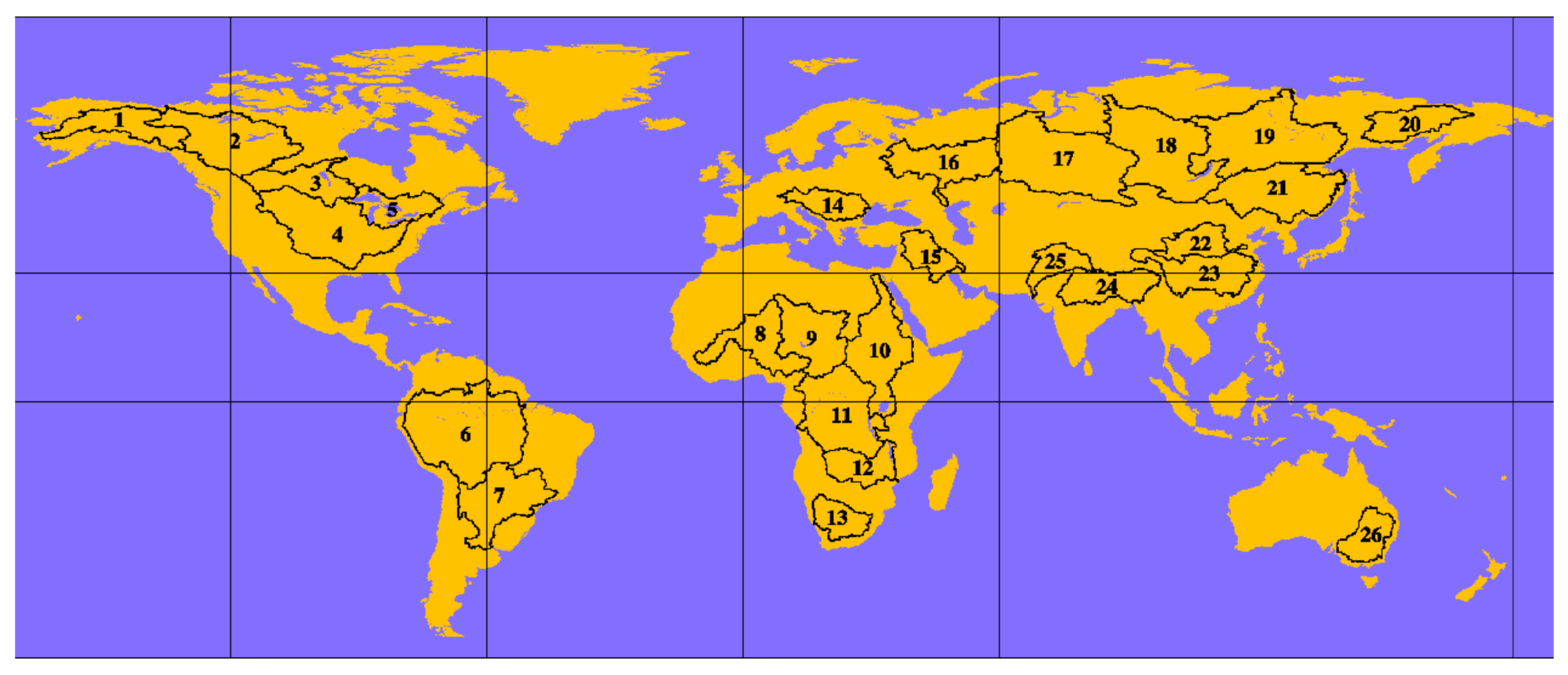
Based on the optimal data processing strategy of the Swarm model for detecting water storage variability in terrestrial areas obtained in Section 3.1, Swarm-TWSC was calculated for 26 areas and compared with GRACE-TWSC in terms of correlation coefficient and root mean square error to evaluate the capability of the Swarm model for water storage detection.

The magnitude and accuracy of Swarm’s water storage potential are closely related to the characteristics of the area under study. To this end, this paper is based on water storage trends detected by the GRACE time-varying gravity field model for 26 major global basins between December 2013 and June 2017, i.e., GRACE-TWSC, and the basin area, average annual runoff within the basin, and annual and instantaneous changes in basin water storage are calculated for each basin. The results can be seen in Figure 7 and

Table 14. Statistical table of water storage change information in 26 basins.

NO	Basin	Area (10,000 km2)	Runoff (km3)	GRACE-Trend (cm/Year)	Average Mass Change (km3)	Swarm-Trend (cm/Year)	Correlation Coefficient (%)	RMSE (cm)
1	Yukon	83.5	200.6	−1.69	−14.11	−0.77	62.44	4.03
2	Mackenzie	180.5	357.2	−1.1	−19.86	0.47	55.97	4.45
3	Nelson	115	74.7	−1.21	−13.91	2.68	−1.62	5.88
4	Mississippi	323	599.5	1.02	32.95	1.64	58.3	3.94
5	St Lawrence	30	332.39	0.9	2.7	2.77	29.14	5.95
6	Amazon	691.5	6906.38	−2.11	−145.91	−2.59	93.55	4.92
7	Parana	310.3	800	2.79	86.57	0.40	42.85	6.29
8	Niger	209	200	−0.26	−5.43	−0.10	58.86	3.12
9	Lake Chad Basin	100	450	−0.23	−5.06	0.50	61	5.43
10	Nile	335	81	−0.6	−20.1	−0.48	70.14	4.38
11	Congo	401	1292.98	−0.07	−2.807	−0.67	57.66	3.46
12	Zambezi	138	311.1	−1.68	−23.18	−0.27	71.56	6.86
13	Orange	102	15.45	−0.2	−2.04	−0.15	5.36	5.65
14	Danube	81.7	203	−0.31	−2.53	1.61	32	4.96
15	Euphrates and Tigris	104.8	62.06	4.91	51.46	−0.87	39.45	4.39
16	Volga	138	254.18	1.43	19.73	1.19	81	3.56
17	Ob	297	385	1.97	58.51	0.86	77.13	3.89
18	Yenisey	260.5	625.36	−0.75	−19.54	−0.62	74.67	3.22
19	Lena	249	540	−0.41	−10.21	−0.5	57.62	4.16
20	Kolyma	64.4	123	0.14	0.90	−0.42	39.37	5.62
21	Amur	185.5	346.5	−0.89	−16.51	0.52	3.64	4.34
22	Huang He	79.5	58	−0.93	−7.39	0.12	−8.31	4.79
23	Yangtze	180	1160	0.75	13.5	−0.33	53.41	4.03
24	Ganges and Brahmaputra	132.6	165.4	−3.09	−40.97	−2.09	73.56	6.05
25	Indus	116.55	207	−0.63	−7.34	−0.65	52.06	4.73
26	Murray Darling	100	5.99	0.63	6.3	−1.58	−1.68	5.26

.

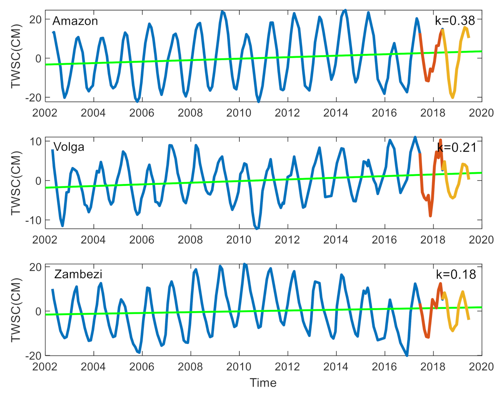
From Figure 7 and Table 14, we can find that the accuracy of Swarm is different in different basins. To get the result more clearly, we analyze it in three aspects which are trend, correlation classification and cycle repetition time. We can get the long-time accuracy of Swarm by compared the TWSC trend with GRACE, get the total accuracy of Swarm by compared the correlation coefficient with GRACE, and get the periodic accuracy of Swarm by summed the similar period with GRACE-TWSC time series.

From the perspective of long-term trends (see Figure 7 and Table 14), Swarm-TWSC and GRACE-TWSC show the same trend of increased and decreased water storage in basins 1, 4–8, 10–13, 16, 17, 19, 24, and 25, and the other basins have the opposite results.

In order to reflect the closeness of the correlation between variables, we use the correlation coefficient in this paper (see

Table 15. Correlation classification.

Correlation Classification	Negative Strongly	Negative Weakly	Irrelevant	Positive Weakly	Positive Strongly
Correlation Coefficient (%)	[−100, 80)	[−80, 30)	[−30, 30]	(30, 80]	(80, 100]

). The correlation coefficient is calculated by the product-difference method based on the deviation of two variables from their respective means, and reflects the degree of correlation between them by multiplying the two deviations. To get the periodic accuracy of Swarm-TWSC in 26 basins, we get the cycle repetition time of each basin between GRACE-TWSC and Swarm-TWSC (see

Table 16. Statistical table of cycle repetition time of 26 basins (December 2012 to June 2017).

NO	Basin	Cycle Repetition Time (Year)	NO	Basin	Cycle Repetition Time (Year)	NO	Basin	Cycle Repetition Time (Year)
1	Yukon	3	10	Nile	3	19	Lena	3
2	Mackenzie	2.5	11	Congo	3	20	Kolyma	2.5
3	Nelson	2.5	12	Zambezi	3	21	Amur	1
4	Mississippi	3	13	Orange	0.5	22	Huang He	0.5
5	St Lawrence	1.5	14	Danube	3	23	Yangtze	2.5
6	Amazon	3.5	15	Euphrates and Tigris	2.5	24	Ganges and Brahmaputra	3
7	Parana	3	16	Volga	3.5	25	Indus	2.5
8	Niger	3	17	Ob	3	26	Murray Darling	1
9	Lake Chad Basin	2.5	18	Yenisey	3

).

From the perspective of correlation coefficient statistics (see

Table 17. Statistics of accuracy indicators of Swarm-TWSC in 26 watersheds.

NO	Basin	Trend	Relevance	Similar Period Ratio
1	Yukon	Same	Positive Weakly	86
2	Mackenzie	Conversely	Positive Weakly	71
3	Nelson	Conversely	Irrelevant	71
4	Mississippi	Same	Positive Weakly	86
5	St Lawrence	Same	Irrelevant	43
6	Amazon	Same	Positive Strong	100
7	Parana	Same	Positive Weakly	86
8	Niger	Same	Positive Weakly	86
9	Lake Chad Basin	Conversely	Positive Weakly	71
10	Nile	Same	Positive Weakly	86
11	Congo	Same	Positive Weakly	86
12	Zambezi	Same	Positive Weakly	86
13	Orange	Same	Irrelevant	14
14	Danube	Conversely	Positive Weakly	86
15	Euphrates and Tigris	Conversely	Positive Weakly	71
16	Volga	Same	Positive Strongly	100
17	Ob	Same	Positive Weakly	86
18	Yenisey	Same	Positive Weakly	86
19	Lena	Same	Positive Weakly	86
20	Kolyma	Conversely	Positive Weakly	71
21	Amur	Conversely	Irrelevant	29
22	Huang He	Conversely	Irrelevant	14
23	Yangtze	Conversely	Positive Weakly	71
24	Ganges and Brahmaputra	Same	Positive Weakly	86
25	Indus	Same	Positive Weakly	71
26	Murray Darling	Conversely	Irrelevant	29

), the region with a strong positive correlation between Swarm-TWSC and GRACE-TWSC is basin 6; the watersheds with weak positive correlation are basins 1, 2, 4–12, 14, 15, 17–20, 23, 24, and 25; and the watersheds that are not relevant are basins 3, 5, 9, 13, 16, 21, 22, and 26.

From Figure 6, we can compare the performance of Swarm-TWSC and GRACE-TWSC in terms of periodicity (see Table 16 and Table 17). By counting the periodic repetition time periods of the two results and calculating their repetition time ratios, we can see that Swarm performs better in basins 1–4, 6–12, 14–20, and 23–25, with the same periodic repetition ratio above 70%, and performs worse in basins 5, 13, 21, 22, and 26.

The long-term trend of water storage changes in land areas is the combination of the two satellite sounding results, and to some extent covers abrupt errors at certain points in time (which can be considered coarse deviations, such as those created by unspecified instrumentation failure, etc.); the correlation between the two results can assess the reliability of the Swarm sounding results. The degree of deviation can measure the accuracy of the Swarm composite value, i.e., the accuracy of the detected water storage height variation value, and the validity of the detection results can be measured by comparing the same length of variation of Swarm-TWSC with the periodic fluctuation of GRACE-TWSC and the increased or decreased time of water storage variation, thus calculating the similar proportion of its periodic variation.

Comparing these three measures, among the 26 major global land basins studied in this paper (see Table 17), we can get the conclusions (Figure 8 and

Table 18. Statistics on the applicability of Swarm-TWSC in 26 basins.

NO	Basin	Result	NO	Basin	Result
6	Amazon	Fully available	25	Indus	Available
16	Volga	Fully available	9	Lake Chad Basin	Applicable
12	Zambezi	Fully available	2	Mackenzie	Applicable
7	Parana	Available	23	Yangtze	Applicable
17	Ob	Available	15	Euphrates and Tigris	Applicable
18	Yenisey	Available	20	Kolyma	Applicable
24	Ganges and Brahmaputra	Available	14	Danube	Applicable
10	Nile	Available	5	St Lawrence	Not available
1	Yukon	Available	13	Orange	Not available
8	Niger	Available	21	Amur	Not available
4	Mississippi	Available	3	Nelson	Not available
11	Congo	Available	26	Murray Darling	Not available
19	Lena	Available	22	Huang He	Not available

), Swarm has the best performance in basins 6, 12, and 16 and the second-best accuracy in basins 1, 4, 7, 8, 10, 11, 17, 18, 19, 24 and 25, and can be used when the GRACE series satellites are not available. Swarm could replace GRACE to detect water storage changes in the above basins. The accuracy of Swarm-TWSC is very bad in basins 3, 5, 13, 21, 22, and 26, so it is not recommended to use the original Swarm satellite time-varying gravity field to recover the water storage changes in these basins. For regions 2, 9, 14, 15, 20, and 23, on the whole, Swarm can detect the periodic change of water reserves certain completely and correctly. However, because the change value of water reserves detected by Swarm may have gross errors at some time points, Swarm-TWSC and GRACE-TWSC have opposite long-term change trends of water reserves. If these gross errors are eliminated, such as basin 2, and if only Swarm-TWSC between 2015 and 2017 is used, the change of water reserves during this period can be detected correctly. Therefore, this paper suggests that the Swarm time-varying gravity field can be selectively used to detect changes in water reserves in these basins if there are no GRACE series satellites or other effective means of detection.

3.3. Reasons for Applying Swarm-TWSC

Swarm satellites have constant accuracy in detecting water storage changes in different basins and different detection capabilities in different basins, which is caused by the different characteristics of the basins. The size of the watershed affects the number of Swarm-TWSC statistical grid points, and the regional water storage variation we obtained is the sum of water storage variation for all grid points. According to statistical theory, in general, the more statistics of equal precision are introduced, the more reliable the results. Therefore, the size of the watershed area affects the accuracy of Swarm detection of regional water storage. In general, the most important factor that causes mass changes in basins is changes in water, and surface water is the main component of the total water, while the size of annual runoff represents the total amount of annual surface water in basins. The quality change of basins detected by Swarm has a certain relationship with the size of runoff, so we also included it in the factors that cause good or bad effects of water storage detection by Swarm. Swarm detects total water storage variation in basins, so it is necessary to analyze this indicator to study the applicability of Swarm. Based on the trend of water storage changes in basins detected by GRACE, the average annual change of water storage can be obtained, combined with the size of the basin, and the applicability of Swarm can be assessed by this indicator. In addition, it is necessary to analyze the degree of water storage change in each basin when assessing the detection capability of Swarm in different basins.

To synthesize the above analysis, in order to evaluate the capability of Swarm to detect water storage changes in terrestrial areas, this paper studied four aspects: area of each watershed, annual runoff volume, annual mass change of water storage, and transient change of water storage, as shown in

Table 19. Statistical table of watershed area, annual runoff, annual change, instantaneous change information and ranking for 26 watersheds.

NO	Basin	Area (10,000 km2)	Rank	Runoff (km3)	Rank	Average Mass Change (km3)	Rank	Instantaneous Change (cm)	Rank	Result Rank
6	Amazon	691.5	1	6906.38	1	−145.91	1	13.66	1	1
16	Volga	138	14	254.18	14	19.73	10	4.61	5	2
12	Zambezi	138	13	311.1	13	−23.18	7	9.96	2	3
7	Parana	310.3	5	800	4	86.57	2	4.83	4	4
17	Ob	297	6	385	9	58.51	3	3.8	8	5
18	Yenisey	260.5	7	625.36	5	−19.54	11	3.38	12	6
24	Ganges and Brahmaputra	132.6	15	165.4	19	−40.97	5	8.94	3	7
10	Nile	335	3	81	21	−20.1	8	3.75	9	8
1	Yukon	83.5	22	200.6	17	−14.11	13	4.22	6	9
8	Niger	209	9	200	18	−5.43	20	1.97	22	10
4	Mississippi	323	4	599.5	6	32.95	6	3.59	10	11
11	Congo	401	2	1292.98	2	−2.81	22	3.02	18	12
19	Lena	249	8	540	7	−10.21	16	2.57	19	13
25	Indus	116.55	16	207	15	−7.34	18	3.1	16	14
9	Lake Chad Basin	100	20	450	8	−5.06	21	3.35	13	15
2	Mackenzie	180.5	11	357.2	10	−19.86	9	2.75	21	16
23	Yangtze	180	12	1160	3	13.5	15	3.15	15	17
15	Euphrates and Tigris	104.8	18	62.06	23	51.46	4	3.06	17	18
20	Kolyma	64.4	25	123	20	0.90	26	3.35	14	19
14	Danube	81.7	23	203	16	−2.53	24	3.83	7	20
5	St Lawrence	30	26	332.39	12	2.7	23	3.47	11	21
13	Orange	102	19	15.45	25	−2.04	25	1.08	26	22
21	Amur	185.5	10	346.5	11	−16.51	12	1.6	24	23
3	Nelson	115	17	74.7	22	−13.91	14	2.69	20	24
26	Murray Darling	100	21	5.99	26	6.3	19	1.76	23	25
22	Huang He	79.5	24	58	24	−7.39	17	1.52	25	26

. The table shows the size and area ranking of each watershed, the size and ranking of annual runoff in each watershed, the size and ranking of overall quality change in each watershed, and the size and ranking of the instantaneous change in water storage in each watershed.

According to the ranking of Swarm detection results, Swarm can be used to detect water storage changes in the first 14 basins. In terms of basin area assessment, there are 11 watersheds in the top 14. Therefore, it can be judged that basin area size is a factor that affects the Swarm detection results. However, it does not mean that the larger the watershed, the stronger the swarm detection ability. For example, watershed 21 ranks 10th in area, but Swarm cannot detect its changes accurately. On the other hand, basin 1 ranks 22nd in area, but it has better Swarm detection results (9th). Therefore, it can be determined that other factors also affect the Swarm detection results.

It can be seen from the influence of annual runoff on Swarm’s detection ability that 9 of the top 14 basins have the best detection effect, which indicates that annual runoff does affect Swarm’s ability to detect regional water reserves. However, similar to the analysis of basin areas, the size of annual runoff is not the only factor that affects the detection results. For example, although the annual runoff of the Yangtze River Basin ranks third, its Swarm detection results were poor (17th), and although the runoff of Nile ranks 21st, its detection results were better (8th).

In analyzing whether the Swarm’s ability to detect regional water reserve changes is related to the total change of annual water reserve of the basin itself, among the basins with a Swarm detection effect, there are 10 in the top 14. Similar to the analysis of the first two factors, the total change of annual water reserve can indeed affect Swarm’s detection ability, but it is not the only factor. For example, the annual change of water reserves in watershed 15 is very large (ranking 4th), but Swarm’s detection effect is poor (18th), and the annual change of water reserves in watershed 11 is small (22nd), but the detection result is good (12th).

The instantaneous change of water reserves in a basin in numerical value is the standard deviation and in graphical form is the amplitude of GRACE-TWSC. According to the statistical results, among the watersheds with good Swarm detection effect, 10 watersheds rank in the top 14 in terms of instantaneous variation of water reserves. Similar to the analysis of the first three factors, the instantaneous change of water reserves can indeed affect Swarm’s detection ability, but it is not the only factor. For example, the annual change of water reserves in watershed 11 is small (ranked 22nd), but Swarm’s detection results are better (ranked 12th), and the instantaneous water reserves in watershed 14 are large (7th), but Swarm’s detection ability is poor (20th).

Combining the above analyses, the four factors all influence Swarm’s ability to detect changes in water storage in basins. In order to quantify the degree of influence of various factors, we calculated the correlation coefficients between the rankings of various factors and the Swarm detection effect so as to count the proportion of influence of the factors on the detection results (see

Table 20. Statistics on the degree of influence of different factors on Swarm-TWSC in 26 watersheds.

	Area	Yearly Runoff	Total Mass Change	Instantaneous Mass Change
Correlation Coefficient (%)	58.75	52.33	60.96	77.8
Impact ratio (%)	23.66	20.99	24.45	31

).

The results show that Swarm detects regional water storage changes on land mainly related to transient changes in regional water storage, followed by total mass change, the area of basins, and finally annual runoff.

3.4. Long-Time GRACE-Swarm-GRACE-FO-TWSC

Based on the results above, we use GRACE, Swarm and GFO to construct the long time series of about 17 years in the Amazon basin, the Volga basin and the Zambezi basin (Figure 9).

The results show that the GRACE-Swarm-GFO-TWSC time series in these three basins with good continuity. The TWSC in the Amazon basin is increased by 0.38 cm per year, in the Volga basin is 0.21 cm per year and 0,18 cm per year in the Zambezi basin.

4. Discussions

In this paper, we first calculated seven GRACE-TWSCs based on seven GRACE time-varying gravity field models, and then used the weighted average method to obtain the time series of water storage changes in 26 major basins around the world to represent the true values of regional water storage changes. Although each GRACE model was checked for accuracy and can be used to detect regional TWSC, there are differences among the seven results and it is difficult to say which model is the best. In this paper, in order to explore the potential of Swarm to detect water storage, we tried to find a GRACE-TWSC with the highest accuracy as the true value, so a weighted average method was used to determine the average of the seven models’ results. Although this approach may weaken the accuracy of the optimal model for part of the time period, it takes into account the combined detection capability of the seven results as much as possible, which is more convincing for multiple regions and long time periods.

Based on the data processing experience of GRACE-TWSC, the optimal filter radius, truncation order, coefficient replacement method, and filtering method of the two Swarm models were analyzed for Swarm-TWSC, and the results show that the optimal data processing strategy is to replace the COST model of order 10 with the C_1,0 term of the SLR model when the Swarm model is used to detect water storage changes in land areas, and then use 1000 km Gaussian filtering. This conclusion is different from the classical data processing strategy of using the GRACE model to detect water storage changes, which may be related to the different principles, satellite configurations, satellite trajectories, and measurement accuracy of the two satellites in measuring the Earth’s time-varying gravity field.

Based on the optimal data processing strategy of the Swarm time-varying gravity field model, Swarm-TWSC was calculated for 26 basins and compared with GRACE-TWSC, and the applicability of Swarm in detecting water storage changes in each basin was analyzed by comparing several accuracy indices (correlation coefficient, root mean square error, and period repetition rate) to determine the credibility of Swarm-TWSC in each basin. The results demonstrate that Swarm-TWSC is fully usable in 3 of the 26 basins worldwide, usable in 11, appropriately usable in 6, and not usable in 6. In this paper, the overall water storage changes in the whole basin are analyzed, but not from a spatial perspective; however, this conclusion does not hinder the utility of reference for other scholars.

Based on the accurate performance of Swarm in detecting water storage changes in 26 watersheds around the world, this paper conducted a statistical analysis in four aspects, watershed area, runoff magnitude, total annual mass change, and transient change, and found that the accuracy of Swarm-TWSC is related to all four factors, with the transient change of watershed mass as the main factor. This finding is convenient for scholars to compare the usability of Swarm when they use it for other studies of new areas.

In this paper, only Swarm-TWSC is compared with GRACE-TWSC, because both exploration models essentially represent water storage changes calculated using a time-varying gravity field model from satellite measurements, and in terms of results, both calculate the total regional mass change. In summary, this paper gives an optimal data processing strategy to systematically explore the potential of Swarm in detecting regional water storage changes and analyzes the reasons for the differences in its performance accuracy in different basins. This paper provides some guidance for future research on Swarm in water storage detection.

Although some conclusions have been obtained in the study of TWSC in 26 basins or other regions, there are still some shortcomings. For the regions with insufficient precision of Swarm-TWSC, the next step is to use GRACE-TWSC as the true value to explore the correlation with Swarm-TWSC, and establish the system difference model of the two types of satellite detection results according to the correlation, then the accuracy of swarm TWSC can be improved.

5. Conclusions

With global climate change, extreme climate disasters and desertification are becoming more and more serious. Therefore, it is of great significance to carry out long-term continuous monitoring of total water storage change. Previous studies are mostly based on the GRACE or GRACE-FO model to restore the change of water reserves, but because there is a gap between the two detection results, they are unable to build a continuous total water storage change time series. Based on this, this paper introduces a Swarm time-varying gravity field model to fill the gap.

First of all, in order to get the optimal results of detecting total water reserves based on the Swarm time-varying gravity field model, this paper evaluates the results of the two models from four aspects: the optimal filtering radius, the optimal model order, the optimal coefficient replacement and the optimal filtering method. It is found that the optimal swarm data processing strategy is to replace the C_1,0 term of the COST model of order 10 with the C_1,0 term of the SLR model, and then do 1000 km Gaussian filtering.

Secondly, based on Swarm’s optimal data strategy, the water storage change time series of 26 basins in the world are calculated and compared with GRACE-TWSC. It is found that Swarm performs differently in different basins. Therefore, in order to accurately detect the potential of Swarm to detect water reserves, this paper discusses the basin area, runoff, annual change and instantaneous change. It is found that the instantaneous change of basins is the main reason affecting the detection accuracy of Swarm.

Finally, taking the Amazon basin, Volga basin and Zambezi basin as examples, combined with GRACE, Swarm and GRACE-FO, a long-term continuous total water storage change time series is constructed.

The research results of this paper will provide a theoretical and results reference for the water storage change research based on Swarm, and have a certain significance for the detection of floods, drought and desertification caused by regional long-term changes of water reserves.

References

1. Tapley, B.D.; Bettadpur, S.; Watkins, M. The gravity recovery and climate experiment: Mission overview and early results. Geophys. Res. Lett. 2004, 31, 4. [Google Scholar] [CrossRef] [Green Version]
2. Li, W.; Guo, J.; Chang, X.; Zhu, G.; Kong, Q. Spatiotemporal variation of land water reserves in Tianshan area of Xinjiang from 2003 to 2013 retrieved by GRACE. J. Wuhan Univ. 2017, 42, 1021–1026. [Google Scholar]
3. Velicogna, I.; Wahr, J. Measurements of time-variable gravity show mass loss in Antarctica. Science 2006, 311, 1754–1756. [Google Scholar] [CrossRef] [PubMed] [Green Version]
4. Velicogna, I.; Wahr, J. Acceleration of Greenland ice mass loss in spring 2004. Nature 2006, 443, 329–331. [Google Scholar] [CrossRef] [PubMed] [Green Version]
5. Chambers, D.P.; Wahr, J.; Nerem, R.S. Preliminary observations of global ocean mass variations with GRACE. Geophys. Res. Lett. 2004, 31, L13310. [Google Scholar] [CrossRef] [Green Version]
6. Lombard, A.; Garcia, D.; Ramillien, G.; Cazenave, A.; Biancale, R.; Lemoine, J.M.; Flechtner, F.; Schmidt, R.; Ishiie, M. Estimation of steric sea level variations from combined GRACE and Jason-1 data. Earth Planet. 2007, 254, 194–202. [Google Scholar] [CrossRef] [Green Version]
7. Voosen, P. Death watch for climate probe. Science 2017, 357, 1225. [Google Scholar] [CrossRef] [PubMed]
8. CSR News. Available online: http://www2.csr.utexas.edu/grace/ (accessed on 5 July 2021).
9. Wang, Z.; Chao, N. Detection of Greenland time-varying gravity field signal by high-low tracking of swarm satellite. Chin. J. Geophys 2014, 57, 3117–3128. [Google Scholar]
10. Lück, C.; Kusche, J.; Rietbroek, R.; Löcher, A. Time-variable gravity fields and ocean mass change from 37 months of kinematic swarm orbits. Solid Earth 2018, 9, 323–339. [Google Scholar] [CrossRef] [Green Version]
11. Meyer, U.; Sosnica, K.; Arnold, D.; Dahle, C.; Thaller, D.; Dach, R.; Jäggi, A. SLR, GRACE and SWARM gravity field determination and combination. Remote Sens. 2019, 11, 956. [Google Scholar] [CrossRef] [Green Version]
12. Li, F.; Wang, Z.; Chao, N.; Feng, J.; Zhang, B.; Tian, K.; Han, Y. Using Swarm cluster to detect drought events in the Amazon basin from 2015 to 2016. J. Wuhan Univ. 2019, 45, 595–603. [Google Scholar]
13. Cui, L.; Song, Z.; Luo, Z.; Zhong, B.; Wang, X.; Zou, Z. Comparison of Terrestrial Water Storage Changes Derived from GRACE/GRACE-FO and Swarm: A Case Study in the Amazon River Basin. Water 2020, 12, 3128. [Google Scholar] [CrossRef]
14. Forootan, E.; Schumacher, M.; Mehrnegar, N.; Bezděk, A.; Talpe, M.J.; Farzaneh, S.; Zhang, C.; Zhang, Y.; Shum, C.K. An Iterative ICA-Based Reconstruction Method to Produce Consistent Time-Variable Total Water Storage Fields Using GRACE and Swarm Satellite Data. Remote Sens. 2020, 12, 1639. [Google Scholar] [CrossRef]
15. Yin, W.; Hu, L.; Zheng, W.; Jiao, J.J.; Han, S.-C.; Zhang, M. Assessing underground water exchange between regions using GRACE data. J. Geophys. Res. Atmos. 2020, 125, e2020JD032570. [Google Scholar] [CrossRef]
16. Save, H.; Bettadpur, S.; Tapley, B.D. High resolution CSR GRACE RL05 mascons. J. Geophys. Res. Solid Earth 2016, 121, 7547–7569. [Google Scholar] [CrossRef]
17. Li, F.; Kusche, J.; Rietbroek, R.; Wang, Z.; Forootan, E.; Schulze, K.; Lück, C. Comparison of Data-driven Techniques to Reconstruct (1992–2002) and Predict (2017–2018) GRACE-like Gridded Total Water Storage Changes using Climate Inputs. Water Resour. Res. 2020, 56, e2019WR026551. [Google Scholar] [CrossRef] [Green Version]
18. Cheng, M.; Ries, J.C.; Tapley, B.D. Variations of the earth’s figure axis from satellite laser ranging and grace. J. Geophys. Res. Solid Earth 2011, 116, 138. [Google Scholar] [CrossRef] [Green Version]
19. Peltier, W.R. Global glacial isostasy and the surface of the ice-age earth: The ice-5g (vm2) model and grace. Annu. Rev. Earth Planet. Sci. 2004, 20, 111–149. [Google Scholar] [CrossRef]
20. Swenson, S.; Wahr, J.; Milly, P.C.D. Estimated accuracies of regional water storage variations inferred from the gravity recovery and climate experiment (GRACE). Water Resour. Res. 2003, 39, 375–384. [Google Scholar] [CrossRef]
21. Wahr, J.; Molenaar, M.; Bryan, F. Time variability of the earth’s gravity field: Hydrological and oceanic effects and their possible detection using grace. J. Geophys. Res. Solid Earth 1998, 103, 30205–30230. [Google Scholar] [CrossRef]
22. Yao, C. Combined Grace and Hydrometeorological Data to Study the Influence of Natural and Human Factors on Regional Water Storage Change; Wuhan University: Wuhan, China, 2017. [Google Scholar]
Figure 1. Location map of 26 regions worldwide (The boundary file is from http://hydroweb.theia-land.fr/?lang=en&basin, accessed on 5 July 2021).
Remotesensing 13 02659 g001
Figure 2. The Swarm-TWSC time series and the long-time trend with different filtering radius and GRACE-TWSC’s in Basin 1. The left one is Swarm from ASI and the right one is Swarm from COST.
Remotesensing 13 02659 g002
Figure 3. The Swarm-TWSC time series and the long-time trend with different order and GRACE-TWSC’s in Basin 1. The left one is Swarm from ASI and the right one is Swarm from COST.
Remotesensing 13 02659 g003
Figure 4. The Swarm-TWSC time series and the long-time trend with different coefficients and GRACE-TWSC’s in Basin 1. The left one is Swarm from ASI and the right one is Swarm from COST.
Remotesensing 13 02659 g004
Figure 5. The Swarm-TWSC time series and the long-time trend with different filtering methods and GRACE-TWSC’s in Basin 1. The left one is Swarm from ASI and the right one is Swarm from COST.
Remotesensing 13 02659 g005
Figure 6. The processing flow of this research. Firstly, get the GRACE-TWSC and GRACE-FO-TWSC, secondly, based on GRACE-TWSC, compared different results from different Swarm models and different postprocessing methods, get the Optimal Swarm-TWSC, thirdly, combined GRACE-TWSC, Swarm-TWSC and GRACE-FO-TWSC, get the GRACE-Swarm-GFO-TWSC.
Remotesensing 13 02659 g006
Figure 7. GRACE-TWSC and Swarm-TWSC time series and long-term (December 2013 to June 2017) trend plots for 26 areas.
Remotesensing 13 02659 g007
Figure 8. The accuracy classification map of water storage change detection in 26 basins by Swarm. Among them, red represents the area where Swarm is fully available, green represents the area where Swarm is available, cyan represents the area where Swarm can be selectively used, and orange line represents the area where Swarm is not available.
Remotesensing 13 02659 g008
Figure 9. The GRACE-Swarm-GFO-TWSC time series and long-term (April 2002 to June 2019) in the Amazon basin, the Volga basin and the Zambezi basin. The blue line is the GRACE-TWSC time series, the red line is the Swarm-TWSC, the orange line is the GFO-TWSC and the green line is the long time TWSC trend of each basin.
Remotesensing 13 02659 g009