Abstract
Inaccurate Synthetic Aperture Radar (SAR) navigation information will lead to unknown phase errors in SAR data. Uncompensated phase errors can blur the SAR images. Autofocus is a technique that can automatically estimate phase errors from data. However, existing autofocus algorithms either have poor focusing quality or a slow focusing speed. In this paper, an ensemble learning-based autofocus method is proposed. Convolutional Extreme Learning Machine (CELM) is constructed and utilized to estimate the phase error. However, the performance of a single CELM is poor. To overcome this, a novel, metric-based combination strategy is proposed, combining multiple CELMs to further improve the estimation accuracy. The proposed model is trained with the classical bagging-based ensemble learning method. The training and testing process is non-iterative and fast. Experimental results conducted on real SAR data show that the proposed method has a good trade-off between focusing quality and speed.
1. Introduction
Synthetic Aperture Radar (SAR) is an active microwave remote-sensing system. SAR has been widely applied to both military and civilian fields due to its all-time and all-weather observation abilities [1]. However, the imaging quality of SAR is usually degraded by undesired Phase Errors (PEs). These PEs usually come from trajectory deviations and the instability of the platform velocity [2]. The uncompensated PEs will cause serious image blurring and geometric distortion of the SAR imagery [3]. The navigation system cannot provide precise information about these motion errors [4]. For high-quality imaging, especially high-resolution imaging, it is important to compensate for these PEs. Autofocus is a data-driven technique, which can directly estimate the phase error from the backscattered signals [5].
In recent decades, many autofocus algorithms have been developed. These methods can be classified into the following three categories: sub-aperture-based, inverse-filtering-based, and metric-optimization-based algorithms. The sub-aperture autofocus algorithm is also called Map Drift Autofocus (MDA) [6]. MDA divides the full-aperture range-compressed data into equal-width sub-aperture data. Each sub-aperture datum is imaged separately to obtain a sub-map. The position offset is determined by finding the position of the cross-correlation peak between sub-maps [7]. The more sub-apertures that are divided, the higher the order of phase error that can be estimated [8]. Thus, the sub-aperture-based algorithms cannot be used to correct high-order phase errors, which are limited by the number of sub-apertures. The original MDA was developed to correct the phase errors in azimuth. Recent works focus on two-dimensional phase-error correction. In [9], the MDA was extended to highly squinted SAR by introducing a squinted-range-dependent map drift estimator to correct the range-variant PEs. In [10], a novel, two-dimensional, spatial-variant MDA is proposed for an unmanned aerial vehicle SAR autofocus.
The Phase Gradient Autofocus (PGA) is a widely utilized, inverse-filtering-based autofocus method [11]. There are four main steps in the PGA algorithm: center shift in dominant scatters, windowing, phase gradient estimation, and iterative correction. The Maximum Likelihood (ML) [12] and Linear Unbiased Minimum Variance (LUMV) [13] are two of the methods utilized to estimate the phase gradient. The PGA method can quickly estimate and correct phase errors of any order through iteration. However, the performance of the PGA algorithm heavily depends on the existence of the isolating dominant scatters on the target [14]. The algorithm will not work in a scene without dominant scatters. In addition, the window width will also affect the performance of the algorithm [15] and should be carefully set. The original PGA method is proposed for spotlight SAR autofocus [16]. When utilized for stripmap SAR, the full aperture data must first be divided into smaller aperture data along the azimuth direction (each sub-aperture size cannot exceed the size of a synthetic aperture) [17,18]. Then, for each sub-aperture data group, apply the PGA algorithm. In [19], a generalized PGA algorithm, which is suitable for use with the backprojection algorithm, is developed. Evers et al. [20] the PGA algorithm is extended for SAR over arbitrary flight paths, including both near-field and bistatic collection geometry.
The metric-optimization-based autofocus algorithms estimate the unknown phase errors by minimizing metrics such as entropy [21,22,23,24], contrast [25,26], or harpness [27,28]. The most commonly used metric-based autofocus method is the Minimum-Entropy-based Autofocus (MEA) method. Usually, the phase error is modeled as a polynomial model to reduce the number of optimization variables [29]. These kinds of algorithm can obtain a higher focusing quality than the above two methods. However, the metric-optimization-based algorithm has high computational complexity and needs a lot of iterations to converge [30]. Moreover, it is difficult to set an appropriate learning rate. Too small a learning rate will lead to an increase in iterations, and too large a learning rate will cause it to converge to a non-optimal solution.
Artificial Neural Network (ANN) is a promising machine-learning technique, used for classification and regression tasks. Extreme Learning Machine (ELM) is a kind of single, hidden-layer, feedforward neural network. ELM was first proposed by Huang et al. [31] in 2004. ELM can also be used to solve the problem of classification and regression [32]. As is widely known, traditional ANN requires thousands of iterative training actions to minimize the objective function. Unlike traditional ANN, the training process of an ELM is non-iterative and very fast. The weights from the input layer to the hidden layer are randomly generated and do not need to be adjusted [33]. The optimization of ELM is used to solve a minimum norm, least squares solution problem, which has a closed-form solution [34]. ELM still has universal classification and approximation abilities and can fit arbitrarily functions [35,36]. In recent years, some ensemble-based ELM methods have been proposed [37,38,39]. Due to its properties of fast training times and a robust performance, ELM is very suitable for ensemble learning.
In this paper, a fast, machine-learning-based autofocus algorithm is proposed. The problem of SAR autofocus can be regarded as regression and prediction of phase error. In order to reduce the regression difficulties, the phase errors are modeled as a polynomial, with a specific degree. The machine learning model is utilized to predict the polynomial coefficients. To deal with the two-dimensional SAR image data, a convolutional extreme learning machine (CELM) is constructed to predict the polynomial coefficients. To improve the performance of a single CELM, multiple individual CELMs are integrated by a novel, metric-based combination strategy. The bagging-based ensemble learning method is utilized to train the model. The main contributions of this paper can be summarized as follows: (1) To the best of our knowledge, this is the first use of machine learning to solve the SAR autofocus problem. (2) A metric-based combination strategy is proposed. (3) A novel SAR autofocus scheme, based on our proposed, ensemble, convolutional, extreme learning machine, is proposed.
The remainder of this paper is organized as follows. In Section 2, the fundamental background of SAR autofocus is explained. Section 3 presents our approach to SAR autofocus. Section 4 describes the dataset, outlines the experimental setup, and presents the results. In Section 5, the results obtained in the performed experiments, the practical implications of the proposed method, and future research directions are discussed. Finally, Section 6 concludes the paper.
2. Fundamental Background
SAR autofocus is a data-driven parameter-estimation technology. It aims to automatically estimate the phase error from the SAR-received data. The residual phase error in the distance direction is generally so small that it can be ignored after the correction of range cell migration. The phase errors that needs to be corrected mainly occur in the azimuth direction [40]. The azimuth phase error estimation and compensation usually occur in the range-doppler domain. Suppose we have a complex-valued defocused image , where are the number of pixels in the azimuth and range, respectively. Denote as the range-doppler domain data matrix of . The one-dimensional azimuth phase error compensation problem can be formulated as [41]
where is the compensated image matrix; k is frequency index in azimuth. are the azimuth and range index subscripts of matrix , respectively. is the k-th element of the phase error vector . Let be a square diagonal matrix composed of the elements of vector on the main diagonal, i.e., , where represents the diagonalization operation. Thus, Equation (1) can be expressed in the form of matrix multiplication as follows:
where represent the Fourier transform and the inverse Fourier transform in azimuth, respectively.
The key problem of autofocus is how to estimate from defocused image . Phase Gradient Autofocus is a simple autofocus algorithm and has been widely used. Denote as a defocused SAR image. First, find the dominant scatters (targets with large intensities) of each range line. Then, center shift these strong scatters along the azimuth direction to obtain a center-shifted image . This method assumes that the complex reflectivites, except for the dominant scatters, are distributed as zero-mean Gaussian random noises [41]. To accurately estimate the phase error gradient from these dominant targets, the center-shifted image is windowed. Denote as the range doppler domain data (apply azimuth Fourier transform to ) of . The phase gradient estimation based on Maximum Likelihood (ML) can be formulated as
where is the complex conjugation of , is the estimated phase error gradient vector, and ∠ is the phase operation. Another commonly used gradient estimation method is Linear Unbiased Minimum Variance (LUMV) algorithm. Let be the gradient matrix of in azimuth, i.e., , where and . The LUMV-based phase error gradient estimation is expressed by
where represents taking the imaginary part of a complex number.
Different from PGA, the metric-based autofocus algorithms estimate phase errors by optimizing a cost function or a metric function. The cost function has the ability to evaluate the focus quality of the image. In the field of radar imaging, entropy is usually used to evaluate the focusing quality of an image. The better the focus, the smaller the entropy. Denote as a complex-valued image; the entropy is defined as
where are the height and width of the image, respectively, is the element in the i-th row and j-th column of amplitude image , ln is the natural logarithm, and scalar can be computed by [24]
Contrast is another metric used to evaluate an image’s focusing quality. In [30], contrast is defined as the ratio of the mean square error of the target energy to the mean value of the target energy
where denotes the mathematical expectation operation. The better the image focus quality, the greater the contrast, and vice versa.
The minimum-entropy based autofocus (MEA) algorithm aims at minimizing
where is the phase error vector, is the compensated image and can be computed using Equation (1). Since C is a constant, minimizing Equation (8) is equivalent to minimizing the following equation
Utilize the gradient descent method, one can optimize Equation (9); the iterative update formula can be expressed as
where is learning rate, is the updated phase error vector, is iteration counter, and is the maximum iteration number.
The partial derivative of with respect to can be formulated as
where . According to [24], the final expression is
where can be calculated by azimuth Fourier transform
In general, for different types of phase error, can be modeled in different forms. Modeling can reduce the number of parameters that need to be optimized and the complexity of the problem. In this paper, we focus on the polynomial type phase error, which can be formulated as
where is the azimuth frequency vector, which can be normalized to or , is the polynomial coefficient vector and Q is the order of the polynomial.
The minimum-entropy-based methods are not restricted by the assumptions in PGA, but require many iterations to converge. As a result, these methods are more robust than PGA, and have a higher focus quality, but suffer from slow speed. In this paper, we focus on the development of a non-iterative autofocus algorithm based on machine learning. An ensemble-based, machine-learning model is proposed to predict the polynomial coefficients. The azimuth phase errors are computed according to Equation (14). The SAR image can be focused by compensating for the errors in azimuth using Equation (2).
3. Materials and Methods
In this section, ensemble learning and extreme learning machine are briefly introduced, and the proposed ensemble-learning-based autofocus method is described in detail.
3.1. Ensemble Scheme
Ensemble learning combines some weak but diverse models with certain combination rules to form a strong model. Key to ensemble learning are individual learners with diversity and the combination strategy. In ensemble learning, individual learners can be homogeneous or heterogeneous. A homogeneous ensemble consists of members with a single-type base learning algorithm, such as the decision tree, support vector machine or neural network, while a heterogeneous ensemble consists of members with different base learning algorithms. Homogeneous learners are most commonly used [42].
Classical ensemble methods include bagging, boosting, and stacking-based methods. These methods have been well-studied in recent years and applied widely in different applications [43]. The key idea of a boosting-based algorithm is: the samples used to train the current individual learner are weighted according to the learning errors of the previous individual learner. Thus, the larger the errors in a sample used by the previous individual learner, the greater the weight that is set for this sample, and vice versa [44]. Therefore, in the boosting-based algorithm, there is a strong dependence among individual learners. It is not suitable for parallel processing and has a low training efficiency. The bagging (bootstrap aggregating) ensemble method is based on bootstrap sampling [37]. Suppose there are training samples and M individual learners; then, N samples are randomly sampled from the original samples to form a training set. M training sets for M individual learners can be obtained by repeating M times sampling. Therefore, in the bagging-based method, there is no strong dependence between individual learners, which makes it suitable for parallel training. In this paper, the bagging-based ensemble method is utilized to form data diversity.
In ensemble learning, three combination strategies have been widely used, including averaging, voting, and learning-based strategies [45]. For the regression problem, the first method is usually utilized, i.e., averaging the outputs of M individual learners to obtain the final output. The second strategy is usually used for classification problems. The winner is the candidate with the maximum total number of votes [46]. The learning-based method is different from the above two methods; it takes the outputs of M individual learners as the inputs of a new learner, and the combination rules are automatically learned. To combine the results of multiple individual autofocus learners, we propose a metric-based combination strategy. In other words, the winner is the candidate with the optimal metric value (such as minimum-entropy or maximum-contrast. The framework of our proposed ensemble-learning-based autofocus algorithm is illustrated in Figure 1, where “PEC” represents the phase error compensation module, which is formulated by Equation (2).
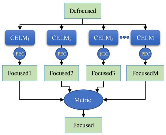
Figure 1.
The framework of our proposed ensemble-learning-based autofocus algorithm.
In Figure 1, there are M homogeneous individual learners. Each learner is a Convolutional Extreme Learning Machine (CELM). Denote as a defocused SAR image, where are the number of pixels in azimuth and range, respectively. We can obtain M estimated phase errror vectors . These vectors are used to compensate for the defocused image , and M focused images are obtained. Finally, our proposed metric-based combination strategy is applied to these images to obtain the final result. For example, if entropy is utilized as the metric, then the final focused image can be expressed as
Similarly, if contrast is utilized as the metric, then the final focused image can be expressed as
3.2. Convolutional Extreme Learning Machine
The original ELM is a three-layer neural network (input, hidden, output) designed for processing one-dimensional data. Denote as the input vector, and L as the number of neurons in the hidden layer. Let represent the weight between input and the i-th neuron of hidden layer, and let be the bias. The output of the i-th hidden layer neuron can be expressed as
where g is a nonlinear piecewise continuous function (activation function in traditional neural networks). The L outputs of the L hidden layer neurons can be represented as , where .
Denote as the weight, ranging from the hidden layer to output layer; K is the number of neurons in the output layer. For a classification problem, K is the number of classes; for a regression problem, K is the dimension of the vector to be regressed. The output of ELM can be formulated as
Suppose there is a training set with N training samples: , where is the truth-value vector (for the classification problem, is the one-hot class label vector). The hidden layer feature matrix of these N samples is . The classification or regression problem for ELM is to optimize
where , is the regularization factor, is the truth-value matrix of the N samples.
Equation (19) can be solved by an iterative method, orthogonal projection method or singular value decomposition [34,47]. When , Equation (19) has the following closed-form solution [32]
where is an identity matrix. The process of solving does not need iterative training, and it is very fast.
The original ELM can only deal with one-dimensional data. For two-dimensional or a higher dimensional input, it is usually flattened to a vector. This flattened operation destroys the original spatial structure of input data and leads ELMs to perform poorly in image-processing tasks. To overcome this problem, Huang et al. [48] proposed a Local Receptive-Fields-Based Extreme Learning Machine (ELM-LRF). Differing from the traditional Convolutional Neural Network (CNN), the size and shape of the receptive field (convolutional kernel) of ELM-LRF can be generated according to the probability distribution. In addition, CNN uses a back-propagation algorithm to iteratively adjust the weights of all layers, while ELM-LRF has a closed-form solution.
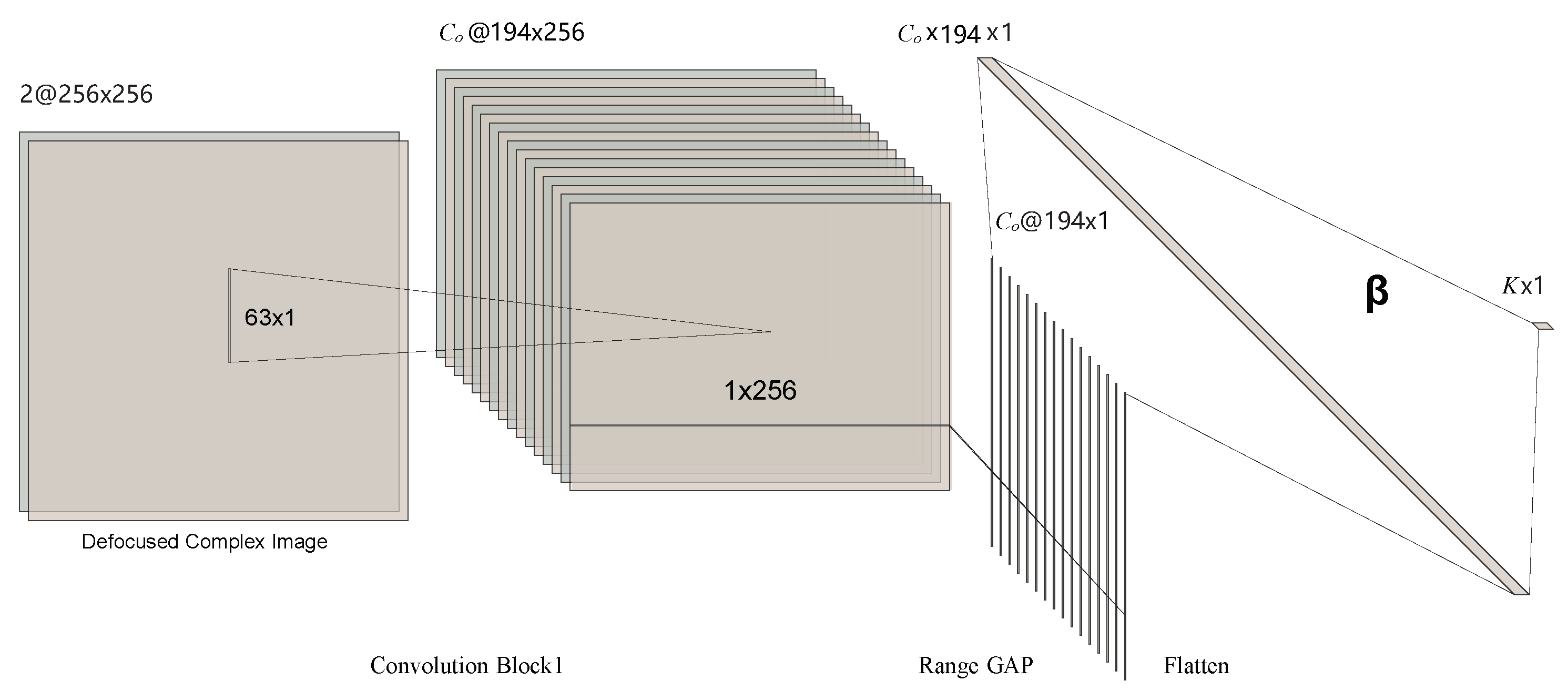
In this paper, we propose a Convolutional Extreme Learning Machine (CELM) method for phase error estimation. The network structure of a single CELM is illustrated in Figure 2. It contains a convolutional (Conv) layer, an Instance Normalization (IN) layer [49], a Leaky Rectified Linear Unit (LeakyReLU) nonlinearity [50], a Global Average Pooling (GAP) layer in range, a flattening layer, and an output layer. As mentioned above, in order to simplify the prediction problem, we use CELM to estimate the polynomial coefficients instead of phase errors. In Figure 2, K denotes polynomial coefficients and equals , where Q is the order of the polynomial.
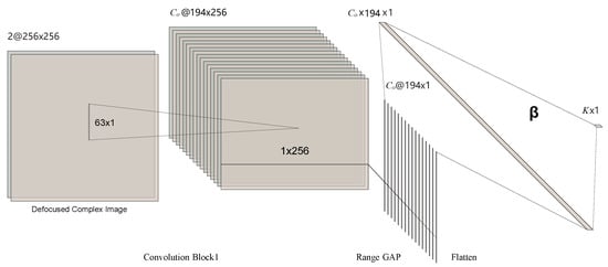
Figure 2.
The structure of a single convolutional, extreme-learning machine for autofocus. The CKS in azimuth is set to 63; the convolution stride is 1.
The detailed configuration of CELM is shown in Table 1. Suppose there is a complex SAR image of 256 pixels in both height and width. Denote as the number of channels produced by convolution, and n as the number of images in a batch. The output size of each layer in CELM is also displayed in Table 1. As shown in Figure 2 and Table 1, there is only one convolutional layer in a CELM. The convolution stride is set to 1. In Figure 2, the convolution kernel sizes for azimuth and range are 63 and 1, respectively.

Table 1.
Configuration of a single convolutional, extreme-learning machine.
Let be convolution input, where N is the number of inputs, and are the height, width and channels of , respectively. In this paper, the convolution kernels between channels do not share weights. Denote as the weight matrix of the convolution kernels, where are the height and width of the convolution kernel. is the number of channels produced by the convolution. The convolution between and can be formulated as
where , * represents the classic two-dimensional convolution operation, and is the -th channel of the n-th image of , and . In this paper, equals 2, since the defocused complex-valued SAR image is first converted into a two-channel image (real channel image and imaginary channel image) before being fed into CELM. As the phase distortion is in azimuth, we use azimuth convolution to extract features. Thus, the weight of the convolutional layer is a matrix with size , where is the number of channels produced by the convolution, 2 is the number of channels of the input image, is the kernel size in azimuth.
The instance normalization of convolutional features can be expressed as
where are the channels, height, and width of , respectively. The mean value and standard variance can be calculated by
After convolution and instance normalization, a LeakyReLU activation is applied to the normalized features . Mathematically, the LeakyReLU function is expressed as
where is the negative slope, set to 0.01 in this paper. Denote as output features of the LeakyReLU nonlinearity. By appying the GAP operation to in the range direction for dimension reduction, the features after pooling can be expressed as
where is the features after the range GAP. Thus, each feature map is reduced to a feature vector. For an image, feature vectors will be generated. These feature vectors are flattened to a long feature vector after the flatten operation. Combine the N feature vectors into a feature matrix
Similar to ELM-LRF, the convolution layer weights are fixed after random initialization. The weights from hidden layer to the output (polynomial coefficients) can be solved by Equation (20).
3.3. Model Training and Testing
In this paper, the classical bagging ensemble-learning method is applied to generate diverse data and train CELMs. The model trained with the bagging-based method is called Bagging-ECELMs. Suppose there is a training dataset , and a validation dataset , where is the n-th defocused image, is the polynomial phase error coefficient vector of , and and are the number of pixels in azimuth and range, respectively. Denote M as the number of CELMs. In order to train the M CELMs, N samples are randomly selected from the training set as the training samples of a single CELM, and M training sets are obtained by repeating this process M times. The validation dataset was utilized to select the best factor in Equation (19). Assuming that there are regularization factors are set in the experiment, then each CELM will be trained times.
The training of a single CELM consists of two main steps: randomly initializing the input weights (the weights of the convolution layer) and calculating the output weights (Equation (20)). The input weights are randomly generated and then orthogonalized using singular value decomposition (SVD) [48]. Assuming that there are convolutional output channels, the convolution kernel size is , where is the kernel size in the azimuth and 1 is the kernel size in the range. Firstly, generate convolution kernel weights with standard Gaussian distribution. Secondly, combine these weights into a matrix in order
Thirdly, orthogonalize the weight matrix with SVD, and obtain the orthogonalized weight . Finally, reshape the weights into a matrix with size to obtain the final input weights .
The pseudocode for training Bagging-ECELMs is summarized in Algorithm 1, where the entropy-based combination strategy is utilized (Equation (15)). The testing process of Bagging-ECELMs model is very simple; see Algorithm 2 for details.
| Algorithm 1: Training CELMs based on bagging |
|
| Algorithm 2: Testing CELMs |
|
4. Experimental Results
This section presents the results obtained with the proposed autofocus method. Firstly, the used datasets are described in detail. Secondly, implementation details, together with the obtained results, are presented and discussed. All experiments were run in PyTorch1.8.1 on a workstation equipped with an Intel E5-2696 2.3GHz CPU, 64GB RAM, and an NVIDIA 1080TI GPU. Our code is available at https://github.com/aisari/AutofocusSAR (accessed on 25 June 2021).
4.1. Dataset Description
The data used for this work were acquired by the Advanced Land Observing Satellite (ALOS) satellite in fine mode. The ALOS satellite was developed by the Earth Observation Research Center, Japan Aerospace Exploration Agency, began to serve in 2006, and ended in 2011. ALOS is equipped with a Phased Array L-band Synthetic Aperture Radar (PALSAR).
The PALSAR has three working modes: fine mode, scanning mode and polarization mode. Specific parameters of the PALSAR in fine mode are shown in Table 2, where represents Pulse Repetition Frequency, i.e., sampling rate in azimuth. As shown in Table 2, there are two resolution modes in fine mode: high-resolution (HR) and low-resolution (LR). With high resolution, the azimuth resolution is about 5 m, the slant range resolution is up to 5m, and the ground resolution is about 7 m.
Table 2.
Platform parameters of ALOS PALSAR in fine mode.
Nine groups of SAR raw data were used in the experiment, covering the areas of Vancouver, Xi’an, Heiwaden, Hefei, Florida, Toledo and Simi Valley. More detailed information, containing the scene name, acquisition date, effective velocity () and Pulse Repetition Frequency (PRF), is given in Table 3. All the raw data can be acquired from https://search.asf.alaska.edu/ (accessed on 25 May 2018) by searching the scene name. A world map of the nine areas is available from our code repository.
Table 3.
Detailed information of acquired SAR data.
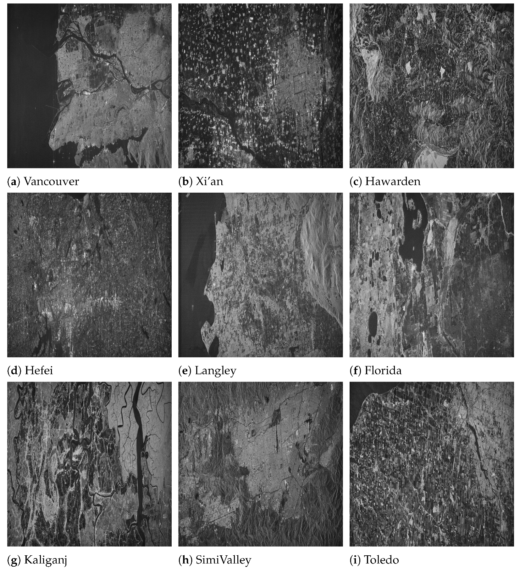
The range doppler algorithm is utilized to process the raw data. Since the original image is very large, we selected a subregion with a size of for each image. The imaging results of the nine sub-images, processed by the range doppler algorithm, are shown in Figure 3. The selected areas include sea surface, urban areas, rural areas, mountains, and other terrains with varying texture complexity, which is an important guarantee for verifying the performance of the autofocus algorithms.
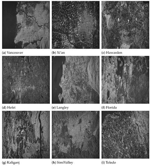
Figure 3.
The SAR images that were utilized to construct the dataset. Each image was imaged by the range doppler algorithm with accurate equivalent velocity. These images are down-sampled to for showing.
We generated azimuth phase errors by simulating an estimation error of equivalent velocity. Of course, the phase errors could also be generated by directly generating polynomial coefficients. The range of velocity estimation error was setatn an interval of 25 , 25 , the sampling interval was 2 , and the range doppler algorithm was used to process imaging. Thus, for every SAR raw data matrix, 25 defocused complex-valued SAR images would be generated. The images corresponding to sequence numbers 2, 3, 4, 5, 8 in Table 3 were used to construct the training dataset. The images corresponding to sequence numbers 6, 7 in Table 3 were used to construct the validation dataset. The images corresponding to sequence numbers 1, 9 in Table 3 were used to construct the testing dataset. Image patches with size were selected from these images to create the dataset. We randomly selected 20,000 image patches for training from the defocused training images. A total of 8000 validation image patches were selected from the defocused validation images. 8000 testing image patches were selected from the defocused testing images.
The entropies of the above unfocused training, validation, and testing images were 9.9876, 10.2911, and 10.0474, respectively. The contrast levels in the above unfocused training, validation, and testing images were 3.3820, 1.9860, and 3.4078, respectively.
4.2. Performance of the Proposed Method
In this experiment, the degree of the polynomial (Equation (14)) was set to ; thus, each CELM had output neurons. AN entropy-based combination strategy was used in this experiment. To analyze the influence of CELMs number on focusing performance, M was chosen from . All CELMs had the same modules as illustrated in Figure 2. The number of convolution kernels was set to . The regularization factor was chosen from . For each CELM, 3000 samples were randomly chosen from the above training dataset to train the CELM. The batch size was set to 10. The NVIDIA 1080TI GPU was utilized to train and testing.
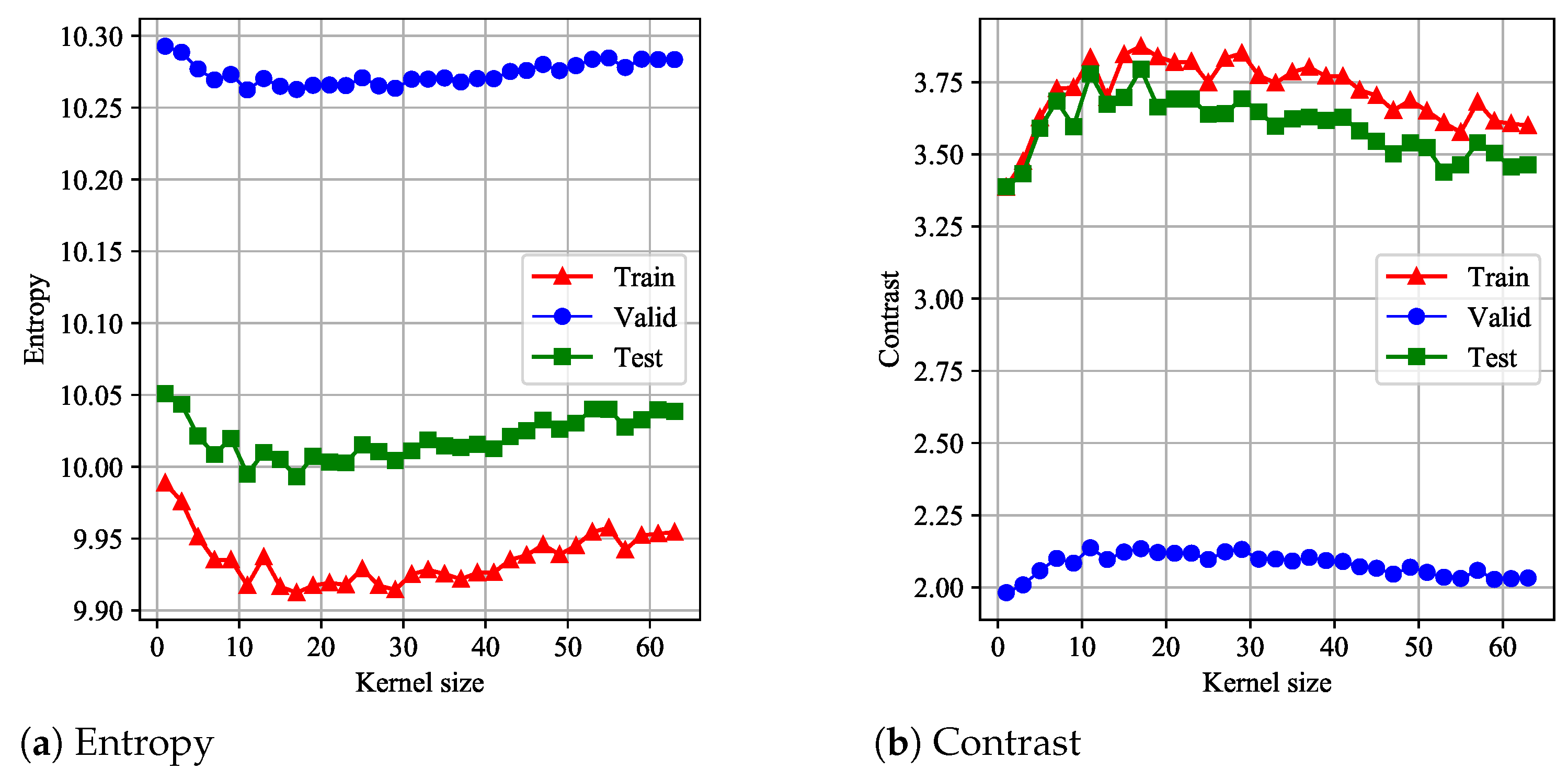
Firstly, we analyzed the influence of convolution kernel size (CKS) on the performance of the proposed model. In this experiment, the number of CELMs was set to 1, and the kernel size in azimuth was chosen from . After training, the entropy and contrast metrics were evaluated on the training, validation, and testing datasets, respectively. The results are illustrated in Figure 4. As we can see from Figure 4a,b, when , the performance was best. The corresponding entropy and contrast on testing dataset were 9.9931 and 3.7952, respectively.
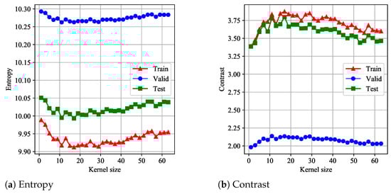
Figure 4.
The focusing performance versus the azimuth kernel size.
Secondly, the influence of the number of CELMs with the same CKS on focusing performance was analyzed. In this experiment, the number of CELMs was chosen from set . The CKS in azimuth of all CELMs were set to 3 and 17, respectively. The training time (see Algorithm 1 for training details.) of the model on the 1080TI GPU device is displayed in Table 4 and Table 5. After training, we tested the trained model on the testing dataset. Then, the entropy, contrast and testing time were evaluated, and the results are shown in Table 4 and Table 5. It can be seen from Table 4 and Table 5 that the higher the number of CELMs, the better the focusing quality, but the focusing time increases. Furthermore, regardless of the number of CELMs, the performance of Bagging-ECELMs with CKS 17 is much better than that of Bagging-ECELMs with CKS 3.
Table 4.
The influence of the number of CELMs with on focusing performance.
Table 5.
The influence of the number of CELMs with on focusing performance.
Thirdly, the influence of the number of CELMs with different CKS on focusing performance is analyzed. Suppose there are M CELMs; the azimuth CKS of the m-th CELM is set as
Equation (28) can generate very different kernel sizes. Here are a few examples: if , then the azimuth CKS are 63 and 31; if , then the the azimuth CKS are 63, 47, 31 and 15; if , then the azimuth CKS are 63, 55, 47, 39, 31, 23, 15 and 7.
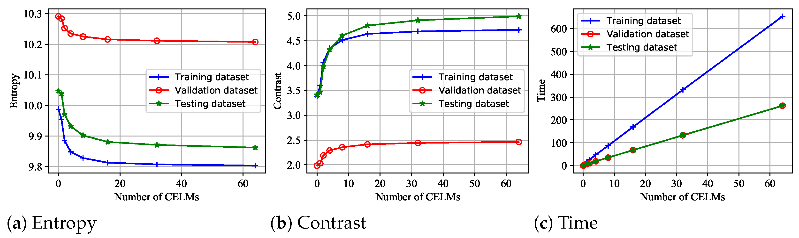
After training all the CELMs, our proposed model is evaluated on the above training, validation, and testing dataset. The results are illustrated in Figure 5 and Table 6.
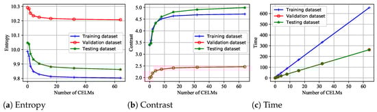
Figure 5.
The focusing performance versus the number of CELMs. The entropy, contrast and time metrics evaluated on the training, validation and testing datasets are illustrated. The kernel size of each CELM is different.
Table 6.
The influence of the number of CELMs with different CKS on focusing performance.
In Figure 5, when the number of CELMs is 0, there is no autofocus. As is known, the smaller the entropy, the greater the contrast, indicating that the focusing quality is better. We can conclude that the higher the number of individual learners (CELMs), the higher the focusing quality. The autofocus time of the proposed model is approximately linear with the number of CELMs. However, when the number of CELMs is large, increasing the number of individual learners has little effect on the focus quality.
The detailed numerical results are given in Table 6. The entropy, contrast and testing (Algorithm 2) time metrics are evaluated on the testing dataset. The training time metric is evaluated on the training and validation dataset; see Algorithm 1 for details. As we can see from Table 6, the training time of the proposed model is directly proportional to the number of individual learners. Comparing the results in Table 4, Table 5 and Table 6 and Figure 4, it can be found that the size of convolution kernel has a great influence on the performance of the model. When the optimal kernel size is unknown, using different kernel sizes can yield more optimal solutions.
Finally, to verify the effectiveness of the proposed combination strategy, the classical average combination strategy, which averages the outputs of M CELMs, is tested. In this experiment, a different CKS is used, which can be computed by Equation (28). The performances with different numbers of CELM in the testing dataset are shown in Table 7. The training time, evaluated on training and validation datasets, is also provided. From Table 6 and Table 7, we can conclude that our proposed entropy-based combination strategy can obtain a higher focus quality. The reason the average method does not work well is that the phase errors predicted by different CELMs may be cancelled out by each other.
Table 7.
The performance of Bagging-ECELMs with average combination strategy.
4.3. Comparison with Existing Autofocus Algorithms
In this experiment, we compared the proposed method with the existing autofocus methods of PGA-ML, PGA-LUMV [16], and MEA [51]. The training, validation and testing datasets described in Section 4.1 were used. In the original PGA algorithm, the window size was set manually. If not set properly, the algorithm will not converge. However, it is difficult to manually set the window size for the above 8000 test images. We implemented an adaptive method to determine the window size. Denote as the complex-valued image data where dominant scatters are center-shifted. The threshold value Tk which determines the window size, is calculated by the following formulas
where are the number of pixels in azimuth and range. Denote as the positions that satisfy and , respectively. Thus, the window size is computed by .
The maximum number of iterations of PGA-ML, PGA-LUMV and MEA are set to 20, 20 and 400, respectively. The tolerance errors of PGA-ML, PGA-LUMV and MEA are both set to 1 × 10. The learning rates of MEA are set to 1, 10 and 100, respectively. The number of CELMs is 64 and the convolution kernel size of CELMs can be computed by Equation (28). The LeakyReLU nonlinear activation function is utilized in all the CELMs. See Section 4.2 for detailed experimental settings.
The results of different autofocus algorithms on the testing dataset are shown in Table 8. In Table 8, MEA-1, MEA-10, MEA-100 represent the MEA algorithms with learning rates 1, 10 and 100, respectively. As is known, the image with lower entropy and higher contrast has a better focus quality. As shown in Table 8, our proposed method and MEA have a better focus quality than PGA-based methods.
Table 8.
The results of different autofocus algorithms on the testing dataset.
In order to intuitively show the focus performance of different methods, three scenes with different texture complexities and defocusing levels were selected in the experiment. Figure 6 shows the autofocus results of the PGA-LUMV, MEA and the proposed autofocus algorithms. It can be seen from the figure that the proposed algorithm and MEA algorithm are suitable for different scenes. However, the phase-gradient-based methods depend on strong scattering points, so PGA-LUMV fails for the scene without strong scattering points, as shown in Figure 6j.
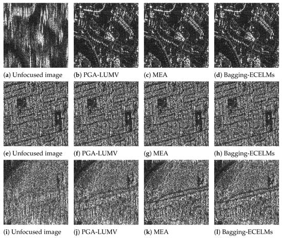
Figure 6.
The focus results of different autofocus algorithms. Three scenes with different defocusing level are illustrated.
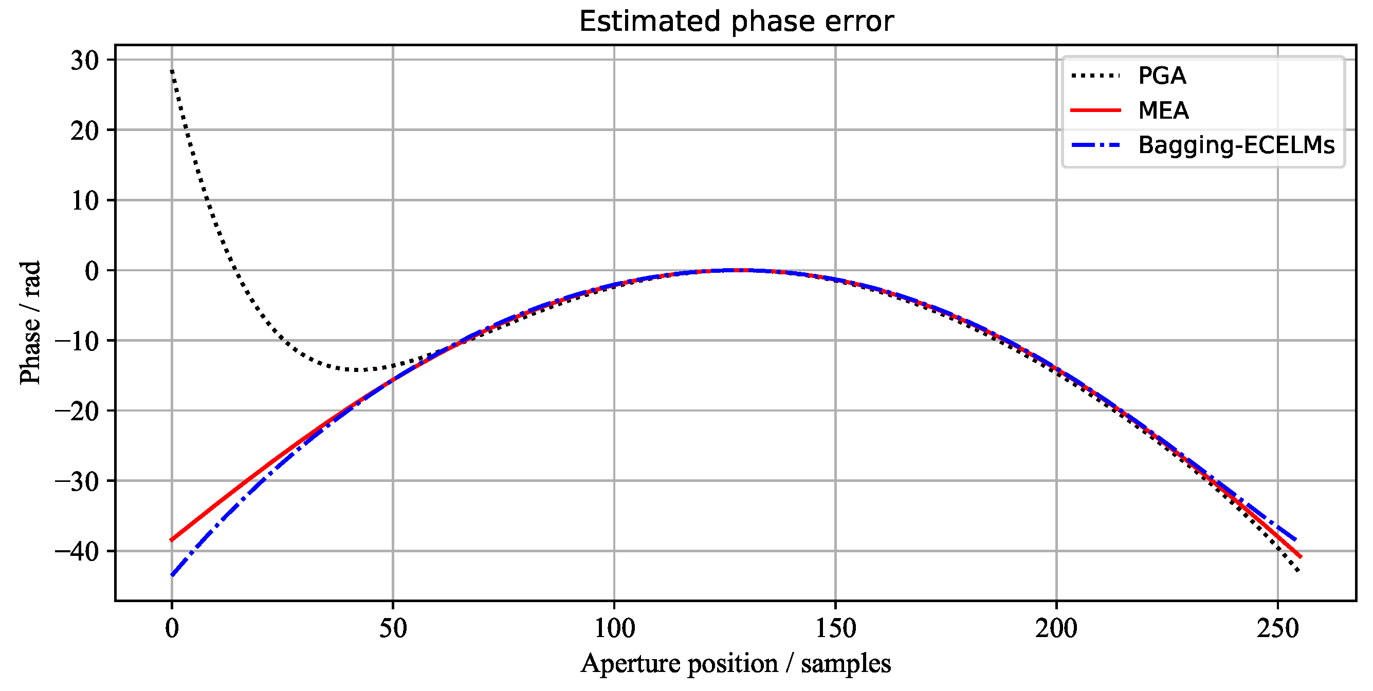
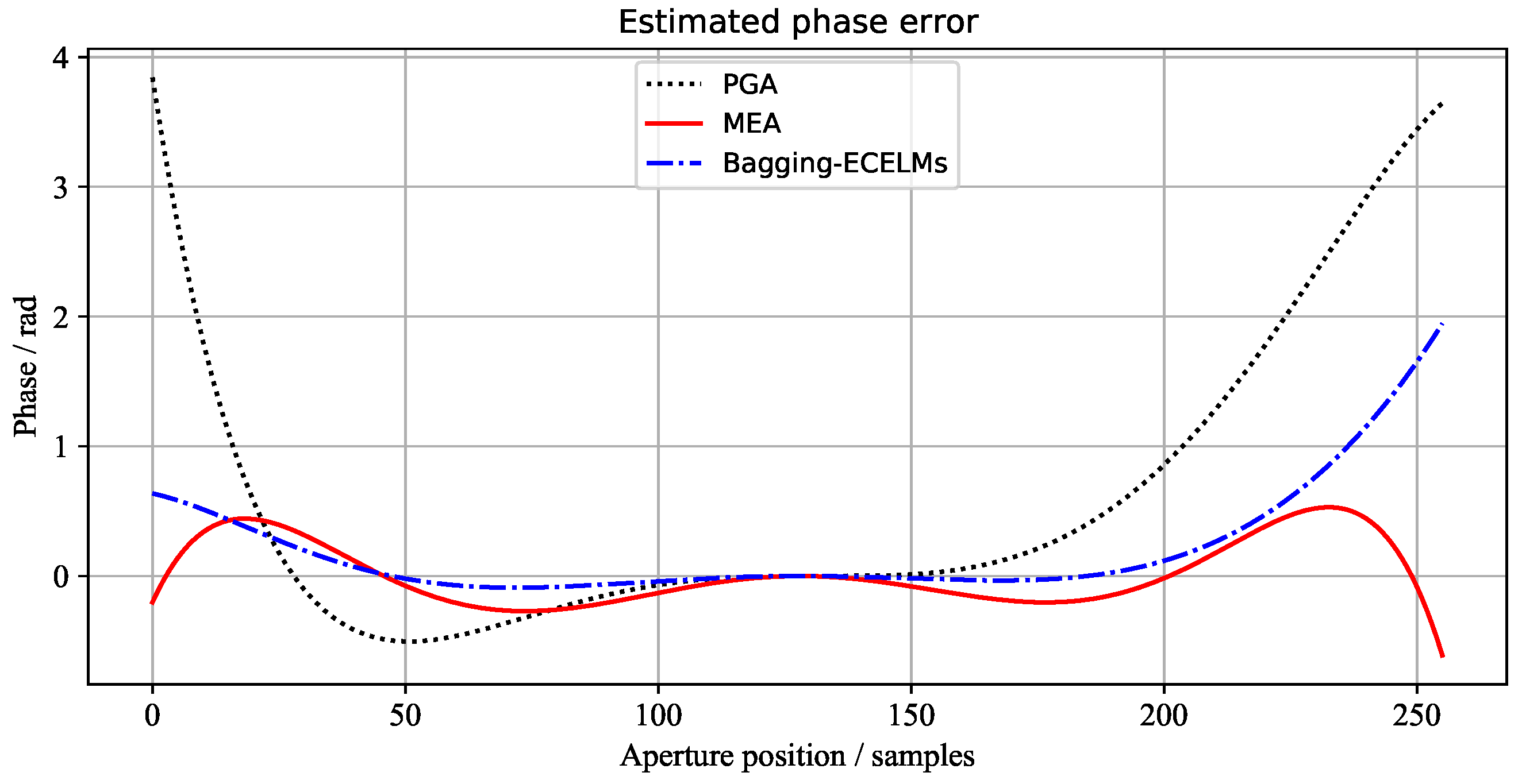
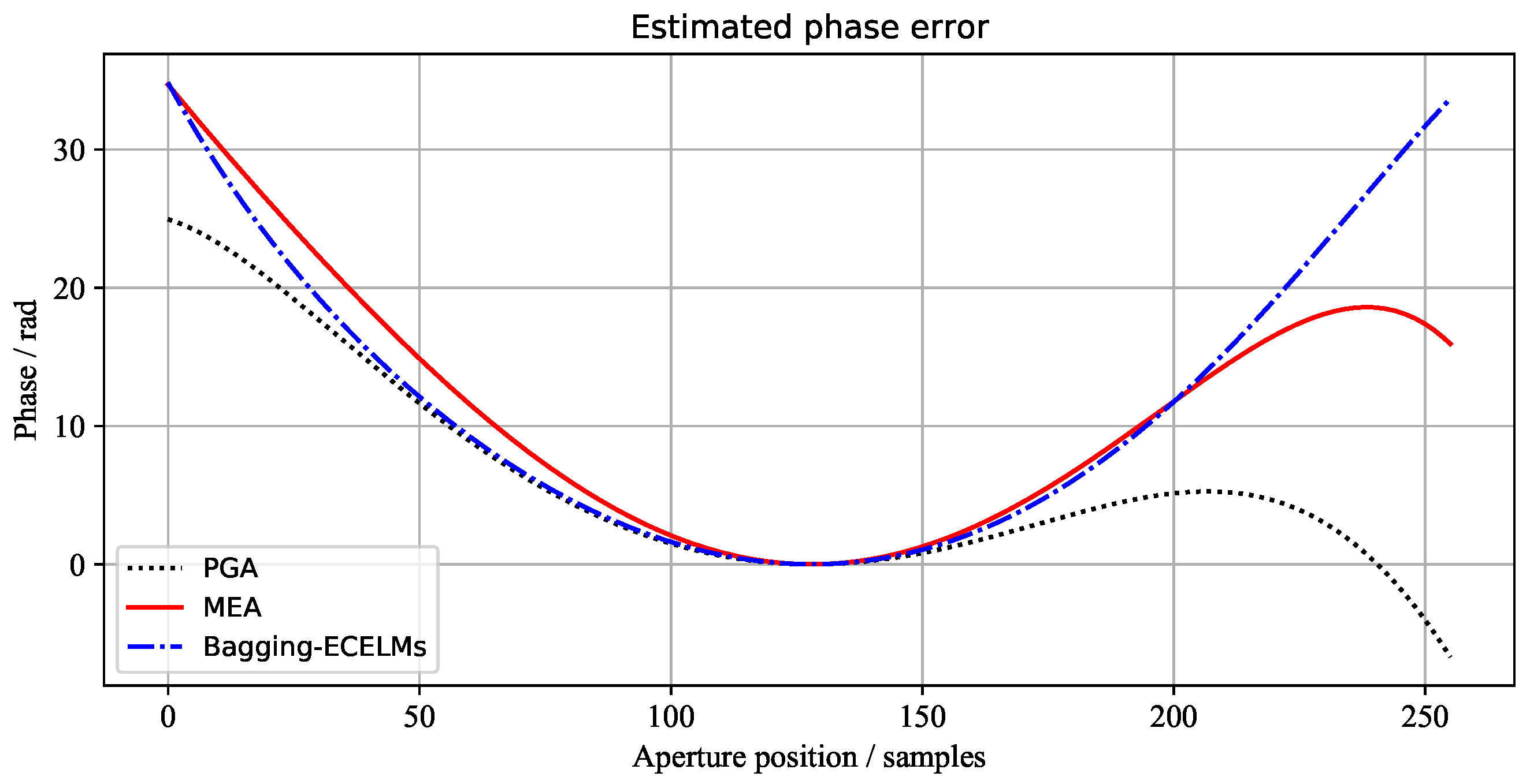
The phase error curves of the three scenes, estimated by the above three methods, are shown in Figure 7, Figure 8 and Figure 9, respectively. It can be seen from Figure 7 and Figure 9 that the 1st image and 3rd image have large phase errors and are seriously defocused. However, the 2nd image has small phase errors. Wecan see that the phase errors estimated by our proposed method are the closest to the results of MEA.
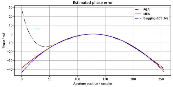
Figure 7.
The azimuth phase error curves of the 1st scene estimated by different algorithms.
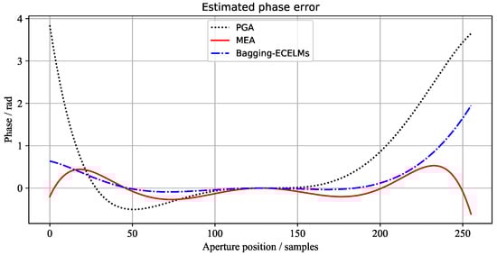
Figure 8.
The azimuth phase error curves of the 2nd scene estimated by different algorithms.
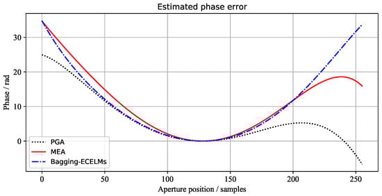
Figure 9.
The azimuth phase error curves of the 3rd scene estimated by different algorithms.
In the experiment, we also evaluated the focus speed of the above four algorithms on a testing dataset. The NVIDIA 1080TI GPU and Intel E5-2696 CPU device were used for these algorithms. The results are shown in Table 9 and Table 10, respectively. It should be noted that the PGA-based algorithms performed more slowly on GPU than on CPU. This is because the center-shifting dominant scatter operations can not be effectively parallelized.
Table 9.
The focusing speed (unit:s) of different autofocus algorithms on GPU.
Table 10.
The focusing speed (unit:s) of different autofocus algorithms on CPU.
It is well-known that PGA has fast convergence and a sufficient performance for low-frequency errors, but is not suitable for estimating high-frequency phase error [41]. Meanwhile, MEA requires more iterations and more time to converge, but can obtain a more accurate phase error estimation. From the results in Table 8, Table 9 and Table 10, we can conclude that our proposed algorithm has a good trade-off between focusing speed and quality.
5. Discussion
SAR autofocus is a key technique for obtaining high-resolution SAR images. The minimum-entropy-based algorithm usually has a high focusing quality but suffers from a slow focusing speed. The phase-gradient-based method has a fast focusing speed but performs poorly (or even does not work) in a scene where a dominant scatterer does not exist. Our proposed machine-learning- and ensemble-learning-based autofocus algorithm (Bagging-ECELMs) has a good trade-off between focusing quality and speed. The experimental results presented in Section 4.3 provide evidence for these conclusions. In Section 4.2, the performance of our proposed method is thoroughly analyzed. Firstly, we found that the convolution kernel;s size has a great influence on the performance of the model. Traversing all convolution kernel sizes is often inefficient and sometimes impossible. Utilizing different kernel sizes can obtain a performance closer to the optimal solutions (see Table 4, Table 5 and Table 6). Secondly, our proposed metric-based combination strategy is much more effective than the classical average-based combination strategy. The phase errors predicted by different CELMs may have different symbols, which will lead to phase error cancellations. Last, but not least, we can easily conclude that our proposed Bagging-ECELMs method performs much better than a single CELM.
However, our proposed Bagging-ECELMs method has the following three disadvantages. Firstly, this model can only be utilized for phase errors that can be modeled as a polynomial. Secondly, a high number of samples is needed for training. Finally, the focusing quality is slightly worse than that based on minimum entropy. Bagging-ECELMs can replace PGA when is used to correct polynomial-type phase errors. When a higher image focusing quality is required and the type of phase error is unknown, the MEA method should be used. The prediction results of Bagging-ECELMs can also be used as the initial values of MEA, to accelerate the convergence speed of MEA. In summary, Bagging-ECELMs is more suitable for real-time autofocus applications, while MEA is more suited to high-quality autofocus applications. Different from MEA and PGA, Bagging-ECELMs is nonparametric at the testing phase and easier to use.
In future research, our work will focus on three aspects. Our proposed algorithm will be extended to correct sinusoidal phase errors. Boosting- or divide-and-conquer-based ECELMs will be developed. Although the method proposed in this paper has a good trade-off between focusing quality and speed, it is still possible to enhance this by improving the combination strategy and network structure.
6. Conclusions
In this paper, we propose a machine-learning-based SAR autofocus algorithm. A Convolutional Extreme Learning Machine (CELM) is constructed to predict the polynomial coefficients of azimuth phase error. In order to improve the prediction accuracy of a single CELM, a bagging-based ensemble learning method is applied. Experimental results conducted on real SAR data show that this ensemble scheme can effectively improve the accuracy of phase error estimation. Furthermore, our proposed algorithm has a good trade-off between focus quality and focus speed. Future works will focus on sinusoidal phase error correction, a novel combination strategy, and developing ECELMs based on boosting or divide-and-conquer. Faster and more accurate SAR autofocus algorithms based on deep learning will also be studied.
Author Contributions
Conceptualization, Z.L. and S.Y.; methodology, Z.L.; software, Z.L.; validation, Q.G., Z.F. and M.W.; formal analysis, Z.L.; investigation, Z.L.; resources, S.Y.; data curation, M.W.; writing—original draft preparation, Z.L.; writing—review and editing, S.Y.; visualization, Z.L.; supervision, S.Y.; project administration, S.Y.; funding acquisition, S.Y. All authors have read and agreed to the published version of the manuscript.
Funding
This research was funded by the National Natural Science Foundation of China under Grant 61771376, Grant 61771380, Grant 61836009, Grant U1701267, Grant 61906145, Grant U1730109, Grant 61703328, Grant 91438201 and Grant 9183830; the Major Research Plan in Shaanxi Province of China under Grant 2017ZDXMGY-103 and Grant 2017ZDCXL-GY-03-02; the Science and Technology Innovation Team in Shaanxi Province of China under Grant 2020TD-017; the Science Basis Research Program in Shaanxi Province of China under Grant 2016JK1823, Grant 2017JM6086 and Grant 2019JQ-663.
Institutional Review Board Statement
Not applicable.
Informed Consent Statement
Not applicable.
Data Availability Statement
Public ALOS SAR data are acquried from https://search.asf.alaska.edu/ (accessed on 25 May 2018).
Acknowledgments
The authors wish to acknowledge the anonymous reviewers for providing helpful suggestions that greatly improved the manuscript.
Conflicts of Interest
The authors declare no conflict of interest.
Abbreviations
The following abbreviations are used in this manuscript:
| ANN | Artificial Neural Network |
| APE | Azimuth Phase Error |
| CELM | Convolutional Extreme Learning Machine |
| CKS | Convolution Kernel Size |
| ELM | Extreme Learning Machine |
| LUMV | Linear Unbiased Minimum Variance |
| MDA | Map Drift Autofocus |
| MEA | Minimum Entropy Autofocus |
| ML | Maximum Likelihood |
| PEs | Phase Errors |
| PGA | Phase Gradient Autofocus |
| SAR | Synthetic Aperture Radar |
| PRF | Pulse Repetition Frequency |
References
- Glentis, G.O.; Zhao, K.; Jakobsson, A.; Li, J. Non-parametric High-resolution SAR Imaging. IEEE Trans. Signal Process. 2012, 61, 1614–1624. [Google Scholar] [CrossRef]
- Yi, T.; He, Z.; He, F.; Dong, Z.; Wu, M.; Song, Y. A Compensation Method for Airborne SAR with Varying Accelerated Motion Error. Remote Sens. 2018, 10, 1124. [Google Scholar] [CrossRef] [Green Version]
- Azouz, A.A.E.; Li, Z. Improved Phase Gradient Autofocus Algorithm based on Segments of Variable Lengths and Minimum-entropy Phase Correction. IET Radar Sonar Navig. 2015, 9, 467–479. [Google Scholar] [CrossRef]
- Shi, H.; Yang, T.; Qiao, Z. ISAR Autofocus Imaging Algorithm for Maneuvering Targets Based on Phase Retrieval and Gabor Wavelet Transform. Remote Sens. 2018, 10, 1810. [Google Scholar] [CrossRef] [Green Version]
- Bezvesilniy, O.; Gorovyi, I.; Vavriv, D. Autofocus: The Key to A High SAR Resolution. In Proceedings of the 2012 International Conference on Mathematical Methods in Electromagnetic Theory, Kharkiv, Ukraine, 28–30 August 2012; pp. 504–507. [Google Scholar] [CrossRef]
- Calloway, T.M.; Jakowatz, C.V., Jr.; Thompson, P.A.; Eichel, P.H. Comparison of synthetic-aperture radar autofocus techniques: Phase gradient versus subaperture. In Proceedings of the Advanced Signal Processing Algorithms, Architectures, and Implementations II. International Society for Optics and Photonics, San Diego, CA, USA, 24–26 July 1991; pp. 353–364. [Google Scholar] [CrossRef]
- Calloway, T.M.; Donohoe, G.W. Subaperture Autofocus for Synthetic Aperture Radar. IEEE Trans. Aerosp. Electron. Syst. 1994, 30, 617–621. [Google Scholar] [CrossRef]
- Yang, R.; Li, H.; Li, S.; Zhang, P.; Tan, L.; Gao, X.; Kang, X. High-Resolution Microwave Imaging; Springer: Singapore, 2018; ISBN 978-981-10-7136-2. [Google Scholar]
- Ran, L.; Liu, Z.; Li, T.; Xie, R.; Zhang, L. Extension of Map-Drift Algorithm for Highly Squinted SAR Autofocus. IEEE J. Sel. Top. Appl. Earth Observ. Remote Sens. 2017, 10, 4032–4044. [Google Scholar] [CrossRef]
- Wang, G.; Zhang, M.; Huang, Y.; Zhang, L.; Wang, F. Robust Two-Dimensional Spatial-Variant Map-Drift Algorithm for UAV SAR Autofocusing. Remote Sens. 2019, 11, 340. [Google Scholar] [CrossRef] [Green Version]
- Yao, Y.; Song, W.; Ye, S. An Improved Autofocus Approach based on 2-D Inverse Filtering for Airborne Spotlight SAR. In Proceedings of the 2016 CIE International Conference on Radar (RADAR), Guangzhou, China, 10–13 October 2016; pp. 1–5. [Google Scholar]
- Jakowatz, C.V.; Wahl, D.E. Eigenvector Method for Maximum-Likelihood Estimation of Phase Errors in Synthetic-Aperture-Radar Imagery. JOSA A 1993, 10, 2539–2546. [Google Scholar] [CrossRef]
- Eichel, P.H.; Jakowatz, C. Phase-Gradient Algorithm as an Optimal Estimator of the Phase Derivative. Opt. Lett. 1989, 14, 1101–1103. [Google Scholar] [CrossRef]
- Zhang, S.; Liu, Y.; Li, X. Fast Entropy Minimization based Autofocusing Technique for ISAR Imaging. IEEE Trans. Signal Process. 2015, 63, 3425–3434. [Google Scholar] [CrossRef]
- Restano, M.; Seu, R.; Picardi, G. A Phase-Gradient-Autofocus Algorithm for the Recovery of Marsis Subsurface Data. IEEE Geosci. Remote Sens. Lett. 2016, 13, 806–810. [Google Scholar] [CrossRef]
- Wahl, D.E.; Eichel, P.; Ghiglia, D.; Jakowatz, C. Phase Gradient Autofocus: A Robust Tool for High Resolution SAR Phase Correction. IEEE Trans. Aerosp. Electron. Syst. 1994, 30, 827–835. [Google Scholar] [CrossRef] [Green Version]
- Thompson, D.G.; Bates, J.S.; Arnold, D.V. Extending the Phase Gradient Autofocus Algorithm for Low-Altitude Stripmap Mode SAR. In Proceedings of the 1999 IEEE Radar Conference. Radar into the Next Millennium (Cat. No. 99CH36249), Waltham, MA, USA, 22–22 April 1999; pp. 36–40. [Google Scholar]
- Callow, H.J.; Hayes, M.P.; Gough, P.T. Stripmap Phase Gradient Autofocus. In Proceedings of the Oceans 2003. Celebrating the Past…Teaming toward the Future (IEEE Cat. No. 03CH37492), San Diego, CA, USA, 22–26 September 2003; pp. 2414–2421. [Google Scholar]
- Evers, A.; Jackson, J.A. A Generalized Phase Gradient Autofocus Algorithm. IEEE Trans. Comput. Imaging 2019, 5, 606–619. [Google Scholar] [CrossRef]
- Evers, A.; Jackson, J.A. Generalized Phase Gradient Autofocus Using Semidefinite Relaxation Phase Estimation. IEEE Trans. Comput. Imaging 2019, 6, 291–303. [Google Scholar] [CrossRef]
- Wang, G.; Bao, Z. The Minimum Entropy Criterion of Range Alignment in ISAR Motion Compensation. In Proceedings of the Radar 97 (Conf. Publ. No. 449), Edinburgh, UK, 14–16 October 1997; pp. 236–239. [Google Scholar] [CrossRef]
- Xi, L.; Guosui, L.; Ni, J. Autofocusing of ISAR Images based on Entropy Minimization. IEEE Trans. Aerosp. Electron. Syst. 1999, 35, 1240–1252. [Google Scholar] [CrossRef]
- Wang, J.; Liu, X. SAR Minimum-Entropy Autofocus using An Adaptive-Order Polynomial Model. IEEE Geosci. Remote Sens. Lett. 2006, 3, 512–516. [Google Scholar] [CrossRef]
- Zeng, T.; Wang, R.; Li, F. SAR Image Autofocus Utilizing Minimum-Entropy Criterion. IEEE Geosci. Remote Sens. Lett. 2013, 10, 1552–1556. [Google Scholar] [CrossRef]
- Berizzi, F.; Corsini, G.; Diani, M.; Veltroni, M. Autofocus of Wide Azimuth Angle SAR Images by Contrast Optimisation. In Proceedings of the IGARSS ’96. 1996 International Geoscience and Remote Sensing Symposium, Lincoln, NE, USA, 31 May 1996; pp. 1230–1232. [Google Scholar] [CrossRef]
- Berizzi, F.; Corsini, G. Autofocusing of Inverse Synthetic Aperture Radar Images using Contrast Optimization. IEEE Trans. Aerosp. Electron. Syst. 1996, 32, 1185–1191. [Google Scholar] [CrossRef]
- Fienup, J. Synthetic-Aperture Radar Autofocus by Maximizing Sharpness. Opt. Lett. 2000, 25, 221–223. [Google Scholar] [CrossRef] [PubMed]
- Morrison, R.L.; Do, M.N.; Munson, D.C. SAR Image Autofocus by Sharpness Optimization: A Theoretical Study. IEEE Trans. Image Process. 2007, 16, 2309–2321. [Google Scholar] [CrossRef]
- Li, J.; Wu, R.; Chen, V.C. Robust Autofocus Algorithm for ISAR Imaging of Moving Targets. IEEE Trans. Aerosp. Electron. Syst. 2001, 37, 1056–1069. [Google Scholar]
- Cai, J.; Martorella, M.; Chang, S.; Liu, Q.; Ding, Z.; Long, T. Efficient Nonparametric ISAR Autofocus Algorithm Based on Contrast Maximization and Newton’s Method. IEEE Sens. J. 2020, 21, 4474–4487. [Google Scholar] [CrossRef]
- Huang, G.B.; Zhu, Q.Y.; Siew, C.K. Extreme Learning Machine: A New Learning Scheme of Feedforward Neural Networks. In Proceedings of the 2004 IEEE International Joint Conference on Neural Networks (IEEE Cat. No. 04CH37541), Budapest, Hungary, 25–29 July 2004; pp. 985–990. [Google Scholar]
- Huang, G.B.; Zhou, H.; Ding, X.; Zhang, R. Extreme Learning Machine for Regression and Multiclass Classification. IEEE Trans. Syst. Man Cybern. B 2011, 42, 513–529. [Google Scholar] [CrossRef] [PubMed] [Green Version]
- Huang, G.B. An Insight Into Extreme Learning Machines: Random Neurons, Random Features and Kernels. Cogn. Comput. 2014, 6, 376–390. [Google Scholar] [CrossRef]
- Bai, Z.; Huang, G.B.; Wang, D.; Wang, H.; Westover, M.B. Sparse Extreme Learning Machine for Classification. IEEE Trans. Cybern. 2014, 44, 1858–1870. [Google Scholar] [CrossRef] [Green Version]
- Huang, G.B.; Zhu, Q.Y.; Siew, C.K. Extreme Learning Machine: Theory and Applications. Neurocomputing 2006, 70, 489–501. [Google Scholar] [CrossRef]
- Huang, G.B.; Chen, L.; Siew, C.K. Universal Approximation Using Incremental Constructive Feedforward Networks with Random Hidden Nodes. IEEE Trans. Neural Netw. 2006, 17, 879–892. [Google Scholar] [CrossRef] [Green Version]
- Liu, N.; Wang, H. Ensemble based Extreme Learning Machine. IEEE Signal Process. Lett. 2010, 17, 754–757. [Google Scholar]
- Cao, J.; Hao, J.; Lai, X.; Vong, C.M.; Luo, M. Ensemble Extreme Learning Machine and Sparse Representation Classification. J. Frankl. Inst. 2016, 353, 4526–4541. [Google Scholar] [CrossRef]
- Duan, M.; Li, K.; Li, K. An Ensemble CNN2ELM for Age Estimation. IEEE Trans. Inf. Forensics Secur. 2017, 13, 758–772. [Google Scholar] [CrossRef]
- Kim, J.W.; Kim, Y.D.; Yeo, T.D.; Khang, S.T.; Yu, J.W. Fast Fourier-Domain Optimization Using Hybrid L1/Lp-Norm for Autofocus in Airborne SAR Imaging. IEEE Trans. Geosci. Remote Sens. 2019, 57, 7934–7954. [Google Scholar] [CrossRef]
- Lee, H.; Jung, C.S.; Kim, K.W. Feature Preserving Autofocus Algorithm for Phase Error Correction of SAR Images. Sensors 2021, 21, 2370. [Google Scholar] [CrossRef] [PubMed]
- Fernández-Alemán, J.L.; Carrillo-de-Gea, J.M.; Hosni, M.; Idri, A.; García-Mateos, G. Homogeneous and Heterogeneous Ensemble Classification Methods in Diabetes Disease: A review. In Proceedings of the 41st Annual International Conference of the IEEE Engineering in Medicine and Biology Society (EMBC), Berlin, Germany, 23–27 July 2019; pp. 3956–3959. [Google Scholar]
- Ren, Y.; Zhang, L.; Suganthan, P.N. Ensemble Classification and Regression-recent Developments, Applications and Future Directions. IEEE Comput. Intell. Mag. 2016, 11, 41–53. [Google Scholar] [CrossRef]
- Polikar, R. Ensemble Learning. In Ensemble Machine Learning; Springer: Boston, MA, USA, 2012; pp. 1–34. [Google Scholar]
- Dong, X.; Yu, Z.; Cao, W.; Shi, Y.; Ma, Q. A Survey on Ensemble Learning. Front. Comput. Sci. 2020, 14, 241–258. [Google Scholar] [CrossRef]
- Leon, F.; Floria, S.A.; Badica, C. Evaluating the Effect of Voting Methods on Ensemble-based Classification. In Proceedings of the 2017 IEEE International Conference on INnovations in Intelligent SysTems and Applications (INISTA), Gdynia, Poland, 3–5 July 2017; pp. 1–6. [Google Scholar]
- Huang, G.B.; Ding, X.; Zhou, H. Optimization Method based Extreme Learning Machine for Classification. Neurocomputing 2010, 74, 155–163. [Google Scholar] [CrossRef]
- Huang, G.B.; Bai, Z.; Kasun, L.L.C.; Vong, C.M. Local Receptive Fields based Extreme Learning Machine. IEEE Comput. Intell. Mag. 2015, 10, 18–29. [Google Scholar] [CrossRef]
- Huang, X.; Belongie, S. Arbitrary Style Transfer in Real-Time with Adaptive Instance Normalization. In Proceedings of the IEEE International Conference on Computer Vision, Venice, Italy, 22–29 October 2017; pp. 1501–1510. [Google Scholar] [CrossRef] [Green Version]
- Maas, A.L.; Hannun, A.Y.; Ng, A.Y. Rectifier Nonlinearities Improve Neural Network Acoustic Models. In Proceedings of the ICML Workshop on Deep Learning for Audio, Speech and Language Processing, Atlanta, GA, USA, 16–21 June 2013; p. 3. [Google Scholar]
- Kragh, T.J.; Kharbouch, A.A. Monotonic Iterative Algorithm for Minimum-Entropy Autofocus. In Proceedings of the Adaptive Sensor Array Processing (ASAP) Workshop, Lexington, MA, USA, 6–7 June 2006; Volume 40, pp. 1147–1159. [Google Scholar]


Publisher’s Note: MDPI stays neutral with regard to jurisdictional claims in published maps and institutional affiliations. |
© 2021 by the authors. Licensee MDPI, Basel, Switzerland. This article is an open access article distributed under the terms and conditions of the Creative Commons Attribution (CC BY) license (https://creativecommons.org/licenses/by/4.0/).