Fire Diurnal Cycle Derived from a Combination of the Himawari-8 and VIIRS Satellites to Improve Fire Emission Assessments in Southeast Australia

Abstract

The violent and persistent wildfires that broke out along the southeast coast of Australia in 2019 caused a large number of pollutant emissions, which seriously affected air quality and the global climate. The existing two methods for estimating combustion emissions based on burned area and fire radiative power mainly use a medium resolution imaging spectrometer (MODIS) on the Aqua and Terra satellites. However, the low temporal resolution of MODIS and insensitivity to small fires lead to deviation in the estimation of fire emissions. In order to solve this problem, the Visible Infrared Imaging Radiometer Suite (VIIRS) with better performance is adopted in this paper, combined with the fire diurnal cycle information obtained by geostationary satellite Himawari-8, to explore the spatio-temporal model of biomass combustion emissions. Using this, a high-spatial- and -temporal-resolution fire emission inventory was generated for southeastern Australia from November 2019 to January 2020, which aims to fully consider the highly dynamic nature of fires and small fires (low FRP) that are much lower than the MODIS burned area or active fire detection limit, with emphasis on dry matter burned (DMB). We found that during the study period, the fire gradually moved from north to south, and the diurnal cycle of the fire in the study area changed greatly. The peak time of the fire gradually delayed as the fire moved south. Our inventory shows that the DMB in southeast Australia during the study period was about 146 Tg, with major burned regions distributed along the Great Dividing Range, with December 2019 being the main burning period. The total DMB we calculated is 0.5–3.1 times that reported by the GFAS (Global Fire Assimilation System) and 1.5 to 4 times lower than that obtained using the traditional “Burned Area Based Method (FINN)”. We believe that the GFAS may underestimate the results by ignoring a large number of small fires, and that the excessive combustion rate used in the FINN may be a source of overestimation. Therefore, we conclude that the combination of high-temporal-resolution and high-spatial-resolution satellites can improve FRE estimation and may also allow further verification of biomass combustion estimates from different inventories, which are far better approaches for fire emission estimation.

1. Introduction

Biomass combustion is an important global source of atmospheric emissions [1,2], which has a significant impact on air quality, climate change and human health [2,3,4,5,6]. Estimating the pollutants emitted into the atmosphere by biomass combustion is very important for studying its impact on air quality and climate change. Greenhouse gases produced by biomass combustion include carbon dioxide, carbon monoxide, methane, nitric oxide and atmospheric particulate matter, etc. [7]. Modeling studies indicate that these emissions can lead to severe regional air pollution events. Huang et al. [8] suggest that PM₁₀ concentrations in some cities may reach 600 ug·m⁻³ during such events, which is six times higher than the WHO 24 h average PM₁₀ air quality guidelines for human health [9]. During the 2019–20 fire season in Australia, the daily concentration of PM2.5 in some densely populated areas exceeded 1000 ug·m⁻³ [6].

Although efforts to quantify emissions from biomass combustion have improved over the past few decades, inaccuracies in input data and differences in methods used can lead to at least 50 percent uncertainty in emission estimates [10,11,12,13]. Early combustion estimates are based on fuel loads, combustion factors and fire return intervals, which vary with vegetation type [14]. While the spatio-temporal variations in fuel load and combustion factor are difficult to assess [10], the method based on remote sensing satellite observation has been paid more and more attention [15]. At present, there are two main methods to estimate biomass combustion emissions based on satellite observations in domestic and foreign studies: (1) method based on burned area [16,17,18,19,20,21,22]; (2) method based on fire radiative power [23,24,25,26,27,28,29,30].

Estimation of biomass combustion emissions based on the burned-area method is the product of the burned area, the density of the above-ground biomass burned, the burning efficiency and the emission factor for each emitted species [16,17,18]. In general, uncertainty in emission assessments arises from all of the above factors. For example, Ito and Penner [19], using the SPOT satellite’s global burned area (GBA) product, estimated that fires emitted 1428 Tg of carbon in 2000. For comparison, Hoelzemann et al. [20], using the ATSR-satellite-generated global burned area product, estimated the carbon for the same year at 1741 Tg. This is surprising, as the estimated GBA by Ito and Penner [19] is almost twice as large as the GLOBSCAR used by Hoelzemann et al. [20]. Korontzi et al. [21] show that estimates of the area burned can vary widely between different acreage burning algorithms, resulting in a more than twofold variation in biomass consumed when the type of land cover being burned is added. This difference has serious influences for accurately quantifying fire emissions [22]. Kasischke and Penner [11] suggested that in addition to the burned area, the difference between fuel load estimation and burning factors is also the reason for the inconsistency in the emission estimations. The difficulty of accurately measuring these variables results in at least 50% uncertainty in emission estimates [10,12,15,21]. Although the dataset for this application is constantly improving, due to the uncertainty of current estimates, it is worth exploring other methods [31,32].

Compared with the traditional method based on burned area, another new promising method based on FRP observed from satellites may bring lower uncertainty to the estimation of combustion emissions. Wooster [23] found that these FRE (fire radiative energy) estimates scale directly to dry matter burned. It is possible to circumvent the uncertainty associated with the estimated burned area, fuel load and burned integrity. In addition, FRP observations can be observed and processed in near real-time [24,25,26]. For example, the GFAS is used to estimate global near-real-time daily fire emissions. The GFAS is currently using the MODIS instrument on the Terra and Aqua satellites for fire observations [25]. Although the method of estimating pollutant emissions based on FRP has achieved relatively good results in many studies [27,28,29,30], the emission inventory based on MODIS is suspected to underestimate pollutant emissions [33,34]. MODIS only provides four observations per day under ideal conditions and has a “bow tie” effect as well as not being sensitive to small fire (low FRP) detection. Although high-spatial-resolution polar-orbit sensors such as VIIRS can provide the ability to identify AFs (active fires) at an increased number and with lower FRP values (, they can still only capture the flames burning in the clear sky at the satellite overpass [34]. Previous studies have found that fire activity exhibits strong Gaussian diurnal cycle characteristics and spatio-temporal variation [35,36,37]. Obviously, due to the highly dynamic nature of fire, the low time resolution of polar-orbiting satellites cannot accurately describe the fire diurnal cycle, which leads to large errors in the process of integrating FRE. Geostationary satellites with high time resolution can make up for the above shortcomings and more accurately capture the changes in the process of fire burning, so as to improve the accuracy of estimating combustion emissions.

This study focuses on a better understanding of the diurnal variation and spatio-temporal dynamic characteristics of fire, so as to improve the estimation results of fire combustion emissions. We use the new fire diurnal cycle information obtained from the geostationary satellite Himawari-8, to reduce the error caused by the low-time-resolution monitoring results of the medium resolution imaging spectrometer. The spatial variation of this fire diurnal cycle and its drivers is discussed in detail and is combined with the twice-daily FRP information provided by the VIIRS product. We aimed to reduce the deviation and uncertainty caused by using only one FRP data type, to take into account the burning even in the short term and to reduce the omission of active fire detection. We used land use data to mask the study area and chose the most suitable smoke emission factor in order to calculate the final total fire emissions based on the estimated value of DMB obtained by FRE.

The paper is organized as follows: Section 2 introduces the study area and data characteristics used in this study. Section 3 introduces the methods of estimating biomass combustion emissions. Section 4 shows the relevant experimental results and comparative analysis. Section 5 concludes with the major findings and problems of this study.

2. Study Area and Data

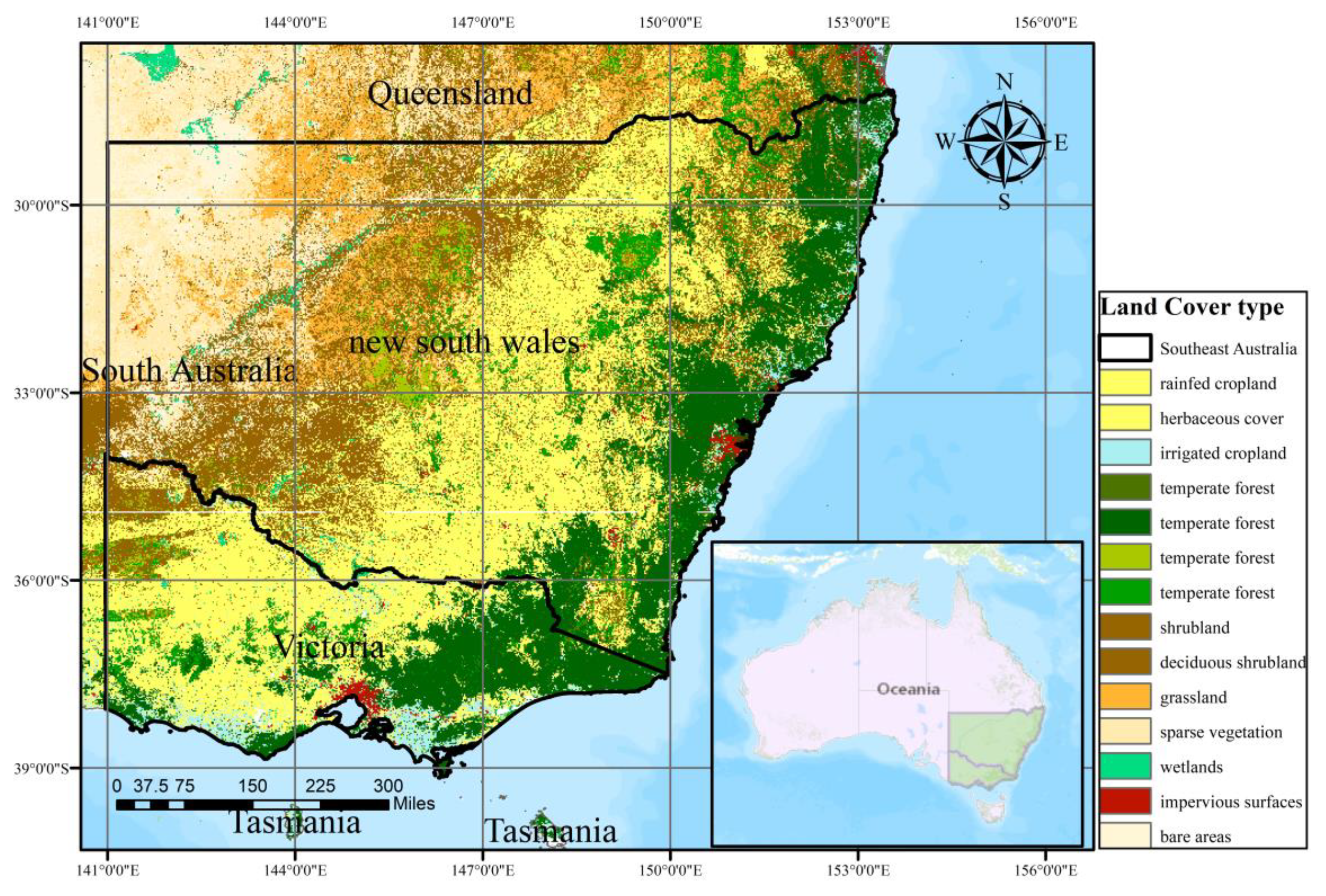
Section 2.1 is a brief description of the study area. Section 2.2 introduces VIIRS data, one of the data sources for estimating emissions, and makes a comparative analysis with MODIS data that is widely used at present. Himawari-8 satellite with higher time resolution for fitting Gaussian Curves is presented in Section 2.3. Land-use-type data used to distinguish different land types is described in Section 2.4. Section 2.5 describes other datasets for validation, such as GFAS and FINN data.

2.1. Study Area

Southeast Australia includes New South Wales and Victoria, with a population of about 3/5 of Australia’s total population, with undulating terrain in the southeast. A vast desert is in the west and the Great Dividing Range is in the east, which runs through southeastern Australia from north to south. Forests are distributed narrowly along the Great Dividing Range, covering about 28.4 million hectares of woodland, accounting for about 18% of the national forest area (Figure 1). The main tree species are eucalypts, high in oil and flammable. Australia has an annual fire season, but since September 2019 wildfires have broken out in many parts of Australia, lasting for a long time and proving difficult to extinguish, covering a total area of more than 6 million hectares. According to the latest annual climate report of 2019 released by the Australian Meteorological Office, the average annual temperature in 2019 was 1.52 °C higher than the record set in 2013 (1.33 °C), and the average maximum temperature was 2.09 °C higher, the highest on record. At the same time, the precipitation was also the lowest on record. In 2019, the entire Australian rainfall was 62% below average, making it the driest spring on record (1967 was the lowest level). Low rainfall has exacerbated pre-existing insufficient rainfall and low soil moisture, and exacerbated meteorological and hydrological drought conditions, meaning that forest fuels are still dry (http://www.bom.gov.au/climate/current/statements/scs72.pdf (accessed June 28,2021).The research period of this article is from 7 November 2019 to 15 January 2020. During this period, the monthly average surface temperature in most parts of the southeast was above 50°C, the monthly average wind speed reached 7 m/s and the coastal temperature was slightly lower (GES DISC (accessed March 15,2021)). High temperature, little rain and strong wind are factors that cause large-scale landscape fires to continue [38].

2.2. Polar-Orbiting VIIRS-IM Fire Radiative Power

The Visible Infrared Imaging Radiometer Suite (VIIRS) instrument onboard the polar-orbiting Suomi NPP (since 2011) and NOAA-20 (since 2017) satellites has transitioned much of the capability of the AVHRR and Moderate Resolution Imaging Spectroradiometer (MODIS) instrument for environmental monitoring [40] (

Table 1. Comparison between MODIS and VIIRS data in sensing geometry.

	MODIS	VIIRS (Suomi NPP)
Orbit altitude	~705 km	~804 km
Equator crossing time	1:30 AM, PM;10:30 AM, PM (local time)	1:30 AM, PM (local time)
Scan angle range	±55°	±56.28°
Swath width	2340 km	3000 km
Pixel dimensions	1 km(nadir)–2.01 km (along track), 1 km(nadir)–4.83 km (along scan)	I-band:375 m(nadir)–800 m (along track), 375 m(nadir)–800 m (along scan) M-band:750 m(nadir)–1.60 km(along track), 750 m(nadir)–1.60 km (along scan)
Primary bands for fire detection and FRP retrieval	B21 (3.929–3.989 μm) B22 (3.940–4.001 μm) B31 (10.780–11.280 μm	I4 (3.550–3.930 μm) M13 (3.987–4.145 μm) M15 (10.234–11.248 μm)

). VIIRS provides a total of 21 bands (plus a day and night band, DNB [41]), spanning from visible light to long-wave infrared, providing better spatial resolution. The nadir pixel resolution is between 375 m and 750 m [42]. The width is 3000 km. Compared with MODIS, VIIRS has a wider bandwidth and provides gapless global coverage [43]. In addition, VIIRS pixels are generated using a pixel aggregation scheme. The samples include: the sample at the lowest point along the scanning direction (scan angle < 31.72°), the sample in the middle area (scan angle: 31.7244.86°) and the sample at the edge of the scan (scan angle > 44.86°). Therefore, the pixel size of VIIRS decreases significantly as the viewing angle increases, and the pixel size is limited to less than four times as the scanning angle increases. When the scanning angle of MODIS changes from the lowest point to the scanning edge, the pixel size along the scanning direction increased by three to nine times [44]. In addition, the VIIRS airborne bow-tie removal algorithm removes two and four over-sampled scan lines in the central gathering area and the scan edge, respectively [45], thereby reducing repeated fire detection between adjacent scans near the lowest point. MODIS does not handle it. VIIRS I4 band (3.55 to 3.93 μm) spans the wavelengths of peak spectral radiance for blackbodies emitted at temperatures between 737 and 817 K, in combination with the improved spatial resolution, the I4 band is therefore well suited for distinguishing pixels of sub-resolution combustion components [46]. Schroeder et al. [46] showed that compared with MODIS AF products, VIIRS AF products have more sensitive “small fire” active detection performance. Due to the relatively low saturation temperature of VIIRS I band, combined with improved spatial resolution, it is easy to cause frequent fire pixel saturation, so it needs to be used in combination with the M band.

2.3. Geostationary Himawari-8 Fire Radiative Power

The new-generation geostationary meteorological satellite Himawari-8 was launched on 7 October 2014. It has 16 observation belts with a spatial resolution of 0.5 or 1 km in visible and near infrared bands, a spatial resolution of 2 km in infrared bands and a temporal resolution of 10 min. It provides data covering the entire global hemisphere of East Asia and Australia, and has provided remote sensing observation data to the world since 2015, including real-time and archived formats. They are available through the official JAXA website. In order to convert a twice-daily VIIRS-IM FRP product into a daily integrated FRE, information on the fire diurnal cycle is required [37,47,48]. Apparently, compared with the observation frequency of the MODIS satellite, four times a day, the high time resolution provided by Himawari-8 can obtain the above information more accurately. However, the spatial resolution of geostationary satellites is relatively coarse, and the presence of mixed pixels increases the deviation of FRP values. Therefore, we combine VIIRS data with higher spatial resolution to reduce the deviation and uncertainty caused by using FRP data alone.

2.4. Land Cover Data

We use the Global 30 m Fine Surface Coverage Product in 2020 [39] to classify land types for the study area in southeast Australia. This dataset is based on the 2015 Global Fine Surface Coverage Product, combined with the time-series surface reflectance data of the Landsat satellite from 2019 to 2020, Sentinel-1 SAR data, DEM terrain elevation data, global thematic auxiliary dataset and prior knowledge datasets, etc., which produced the Global 30 m Fine Surface Coverage Product in 2020. Figure 1 shows the spatial distribution of the land cover in southeast Australia.

2.5. FINN and GFAS Emissions Inventory Data

We used two state-of-the-art global fire emission databases (Fire Inventory from NCAR and Global Fire Assimilation System) to compare the results of this study. FINNv2.2 infers the combustion zone based on MODIS and VIIRS active fire detection data. Since the dataset does not have the combined data of MODIS and VIIRS in 2020, we only use FINNv2.2 based on MODIS data. The FINN assumes that each active fire detection has a pixel area of one square kilometer, and the burning area is further scaled according to the exposed coverage percentage of the VCF (MODIS vegetation continuous field) product at the fire point [49]. FINNv2.2 provides estimates of global fire emissions with a resolution of 1 km per day, including trace gases and aerosols. The emissions are calculated as follows:

$${\mathrm{E}}_{\mathrm{i}}={\mathrm{A}}_{\mathrm{X},\mathrm{t}}\times {\mathrm{B}}_{\mathrm{X}}\times \mathrm{FB}\times {\mathrm{EF}}_{\mathrm{i}}$$

(1)

where E_i is the emission of species i, A_X,t the area burned at location x and moment t, B_X the biomass loading, FB the fraction of that biomass that is burned in the fire (burning ratio) and EF_i the emission factor. The biomass loading is assumed to be based on a specific land cover type, using the estimation method of Hoelzemann et al. [20], and a small number of updates are described by Wiedinmyer et al. [49]. According to the theory found by Ito and Penner [19], the fraction of biomass burned (FB) is related to vegetation cover, which is further described by Wiedinmyer et al. [49,50]., and the emission factor comes from the literature investigation by Akagi et al. [51].

In contrast to the FINN, the GFAS calculates biomass combustion emissions by assimilating fire radiative power observations from the MODIS instruments onboard the Terra and Aqua satellites [52]. The GFAS forms a fire database based on active fire (AF) detection and integrates into the Copernicus Atmosphere Monitoring Service (CAMS) system for near-real-time atmospheric composition monitoring and forecasting. Using the Kalman filtering algorithm developed by Kaiser [25], the FRP data observed by MODIS four times a day are integrated into daily FRE. Then, DMB can be calculated by multiplying FRE by a conversion factor. Finally, DMB is linearly transformed into emission fluxes of 40 smoke constituents (0.1° grid cell) using emission factors derived from field measurements [15].

3. Methodology

The assessment process of pollutants emitted from biomass combustion can be divided into two parts. The first part is the daily FRE generated by the Gaussian curve of the fire diurnal cycle based on the observation results of Himawari-8 and the observation results of VIIRS. The second part is to combine FRE with corresponding emission factors to generate various pollutant emissions.

3.1. Fire Diurnal Cycle and Daily FRE Generation

It has been found from previous studies [27,47] that the diurnal variation of fire has very obvious Gaussian characteristics in a day (0:00–23:00, local time).At present, most of the studies [27,28,29,53] on pollutant emission estimation are based on MODIS FRP fire diurnal cycle fitting. Vermote et al. [27] found that the parameters related to the fire diurnal cycle have a high correlation with the ratio of FRP Terra to FRP Aqua (T/A). However, for some highly dynamic fires, the low time resolution of MODIS obviously has a high error uncertainty, and the correlation between T/A and h (the peak hour of the fire diurnal cycle) is only 0.2. Although Vermote suggested that h has little influence on the final estimated DMB, it is obvious that h is also a source of error.

Here, we represent the fire diurnal cycle as a Gaussian function, parameterized using the Himawari-8 FRP diurnal cycle superimposed on a fixed baseline. Chathura et al. [54] found that the active fire detection ability of Himawari-8 under different FRP is relatively consistent with that of VIIRS. Based on the method of Andela et al. [55], the fire diurnal information obtained by Himawari-8 was mixed with VIIRS data to obtain the parameters related to the fire diurnal cycle. For a given grid cell j at instantaneous time t, the mixed FRP is calculated by:

$${\mathrm{FRP}}_{\mathrm{j},\mathrm{t}}={\mathrm{FRP}}_{\mathrm{j},\mathrm{VIIRS}-\mathrm{night}}+\left({\mathrm{FRP}}_{\mathrm{j},\mathrm{peak}-\mathrm{Him}}-{\mathrm{FRP}}_{\mathrm{j},\mathrm{VIIRS}-\mathrm{hight}}\right){\mathrm{e}}^{-\frac{{\left({\mathrm{t}}_{\mathrm{j}}-{\mathrm{t}}_{\mathrm{j},\mathrm{peak}}\right)}^2}{2{\mathsf{\sigma }}_{\mathrm{j}}^2}}$$

(2)

where FRP_j,t is the instantaneous mixed FRP (MW) for grid cell j at time t, FRP_{j,VIIRS-night} is the night-time (~01:00 LST) VIIRS-IM FRP value for grid cell j, FRP_j,peak-Him is the peak value of the fire diurnal cycle fitted based on the hourly data of Himawari-8 FRP for grid cell j, t_j is the local solar time at time step t, t_j,peak is the local time at which the Himawari-8 FRP diurnal cycle peaks for grid cell j and σ is the standard deviation (dependent on fire duration) of the main peak of the Himawari-8 FRP diurnal cycle calculated by fitting a Gaussian function (using non-linear least squares) to the Himawari-8 FRP diurnal cycles.

For each grid cell j, daily FRE was calculated by:

$${\mathrm{FRE}}_{\mathrm{j}}={{\displaystyle \int }}_0^{23}{\mathrm{FRP}}_{\mathrm{j}}\mathrm{dt}$$

(3)

3.2. Conversion to Smoke Emissions

Wooster et al. found that the relationship between FRE and dry matter burned (DMB) was linear and significant (R² = 0.98), as shown by the following equation [23]:

$${\mathrm{DMB}}_{\mathrm{j}}={\mathrm{FRE}}_{\mathrm{j}}\times \mathrm{CR}$$

(4)

DMB_j is total dry matter burned (kg) for grid cell j, FRE_j represents the fire radiation energy for grid cell j and CR represents the burning conversion ratio (0.368 kg MJ⁻¹ (±0.015 kg MJ⁻¹)) derived by Wooster et al. [23] from a series of outdoor experimental fires. To convert the resultant DMB into smoke emissions, we used the emission factors from Kaiser et al. [25], as is used in the GFAS V1.0 (

Table 2. Emission factors (g kg⁻¹ dry matter residue) for various species emitted in southeast Australia.

Land Cover Class	CO2	CO	PM2.5	BC (Black Carbon)
Temperate forest	1572	106	13.8	0.56
Shrubland	1646	61	4.9	0.46
Agriculture	1308	92	8.3	0.42

). DMB is then multiplied by appropriate particulate and gaseous emission factors in order to estimate the emissions from fire burning.

However, the DMB is obtained according to the Himawari-8 FRP product. The spatial resolution of the land-type cover product used in this study is much higher than that of DMB, so it is necessary to calculate the mixed emission factor of each grid cell. The total area of land use type within each grid cell j was calculated by:

$${\mathrm{A}}_{\mathrm{j}}={{\displaystyle \sum }}_{\mathrm{i}\in \mathrm{j}}{\mathrm{A}}_{\mathrm{i}}$$

(5)

where A_j is the total area of all land-use types in a grid cell j and A_i is the area of the i land-use type in grid cell j.

Mixed emission factors are calculated by multiplying the emission factors of each land-use type by the corresponding area weight in the grid cell and then cumulative calculation:

$${\mathrm{EF}}_{\mathrm{j},\mathrm{mixed}}={{\displaystyle \sum }}_{\mathrm{i}\in \mathrm{j}}\frac{{\mathrm{A}}_{\mathrm{i},\mathrm{i}\in \mathrm{j}}}{{\mathrm{A}}_{\mathrm{j}}}\times {\mathrm{EF}}_{\mathrm{i},\mathrm{i}\in \mathrm{j}}$$

(6)

where EF_j,mixed is the mixed emission factor of grid cell j and EF_i is the emission factor of the i type of land use in grid cell j.

4. Results and Discussions

4.1. Differences in Fire Monitoring

Wooster et al. [56] found that it is difficult for MODIS to detect FRP when below 10 MW, while Schroeder et al. [46] show that VIIRS is more sensitive for small fires. In order to quantify this difference, we compared the spatial distribution of FRP below 10 MW of VIIRS and MODIS Aqua during the study period. For better visualization, FRP is divided into two categories: less than 5 MW and between 5–10 MW. It can be clearly found from Figure 2 that the monitoring result FRP of MODIS Aqua below 5 MW is far worse than that of VIIRS. During the study period, a total number of 269,753 fires with FRP lower than 5 MW were detected by VIIRS, and 2624 fires with FRP lower than 5 MW were detected by MODIS Aqua. 83,900 fire points of FRP between 5–10 MW were detected by VIIRS, and 6387 fire points of FRP between 5–10 MW were detected by MODIS Aqua. Although the spatial resolution of VIIRS is higher than that of MODIS, which means that multiple VIIRS AF pixels may be represented by one MODIS AF pixel, the band feature that VIIRS is sensitive to small fires is the main reason for the higher number of fire pixels than MODIS. Wooster [55] and Ichoku [56] also suggested that low FRP fires are the most common type of fire events at present. If this part is ignored, it may have a significant impact on the estimated results of fire emission pollutants. Obviously, the estimation of fire emission pollutants based on VIIRS has more advantages than on MODIS.

4.2. The Fire Diurnal Cycle Characteristic

The combustion process of the fire is highly dynamic; the study of the variation in characteristics of fire behavior has great value for the accurate estimation of pollutant emissions and future fire extinguishing management. As mentioned in Section 3.1, the diurnal variation of the fire has an obvious Gaussian law [27]; however, there are a few issues in its accurate estimation [28,29]. Therefore, we try to describe the variation in characteristics of fire behavior more accurately by using geostationary satellite Himawari-8.

The parameters of the fire diurnal cycle have been present in the report. The duration and peak time of fire were estimated based on the hourly Himawari-8 FRP time series. Figure 3 shows an example of a grid cell (2 km) in northeastern New South Wales from 7 November 2019 to 11 November 2019, where the last several days of the fire can be seen. The results shown in Figure 3 show that no matter the intensity of the fire, the Gaussian function can describe fire activities well. At the same time, it is also obvious that observations from MODIS sampling intervals did not observe highly dynamic changes in fire well. Based on the method of Vermote et al. [27] described in Section 3.1, we use MODIS data to estimate the duration and peak time of the fire diurnal cycle within five days of the selected grid. Compared with the results obtained from the Gaussian curve fitted with the Himawari-8 data, the method based on MODIS overestimates σ, that is, overestimates the fire duration. In this example, σ is overestimated by about 1–2 h. Moreover, the peak time is also greatly different from the results of Himawari-8, in this case, there is a difference of about 0.5–2 h across each of the five days. The time resolution of Himawari-8 is once every 10 min, so the observation of Himawari-8 is more consistent with the actual fire combustion process, which will make the error smaller in the process of integrating FRP into FRE.

In addition to an observed variability in the fire diurnal cycle seen on different days, we found an interesting spatial distribution in the duration and peak time of fire (Figure 4). We found that the peak time of fire is usually after 14:00 local time. From November 2019 to January 2020, with the southward movement of the fire, the peak time of the fire is gradually later. In November 2019, the peak time of fire was mostly 15:00. In December 2019, the peak time of fire was mostly 16:00. In January 2020, the peak time of fire mainly occurs after 18:00, and the peak time in the early morning was a higher ratio than that in November and December 2019. According to the research of Hély et al. [57], fuel moisture, wind and other ambient atmospheric conditions are far less conducive to intense fire activity by night than by day, therefore, the fire activity at night will generally be significantly reduced. The continuous burning at night in Victoria indirectly reflects the fierce fire in Victoria, which is hard to control. In addition, most σ values are between 1–3.5 h. As mentioned in Section 3.1, the value of σ is determined by the duration of the fire. Compared to December 2019, the fire in northeast New South Wales in November 2019 lasted for a shorter period of time. In December 2019, most of the fires occurred in the central-–eastern and central–southern areas of New South Wales, with a σ value of 2–3 h. As the fire moves to the south, the 0–2 h σ value of January 2020 is much higher than that of November 2019 and December 2019, indicating that there are more short-duration fires in January 2020.

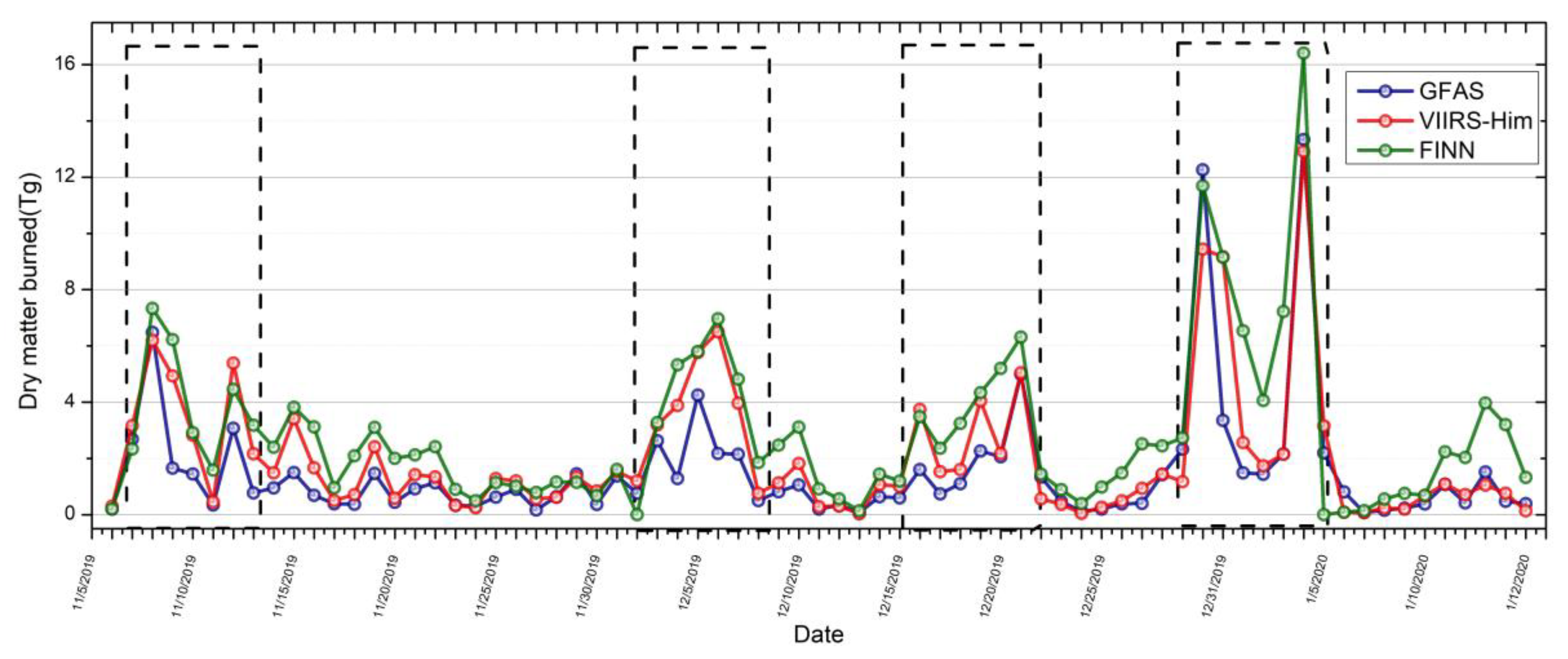
4.3. DMB Comparisons to the FINN and GFAS

The emission estimation results of FRP generated by VIIRS and Himawari-8 are compared with those of the GFAS and FINN. DMB is used as a common comparison indicator because it eliminates the difference in emission factors between different datasets. Overall, compared with the results of the GFAS and FINN, the estimated results of this study are of a very similar consistency with the former two in terms of time variation (Figure 5).

The estimated DMB based on the research method in this paper has four centralized production periods, namely, from 7 November to 13 November 2019, from 3 December to 7 December 2019, from 16 December to 21 December 2019, and from 30 December 2019 to 4 January 2020(

Table 3. The DMB (Tg) produced by four relatively centralized combustion periods.

	7 November 2019–13 November 2019	3 December 2019–7 December 2019	16 December 2019–21 December 2019	30 December 2019–4 January 2020	7 November 2019–4 January 2020
This study	24.82	23.27	18.13	37.97	146.83
GFAS	16.4	12.49	12.75	44.04	129.07
FINN	28.02	26.19	24.94	55.08	204.72

). In the last concentrated production period, 37.97 Tg DMB was produced, accounting for about 26% of the total DMB. The first three concentrated output periods produced 25 Tg, 23 Tg and 18 Tg DMB, respectively. The DMB obtained through this paper during the study period is about 1.13 times higher than that reported by the GFAS. As described in Section 4.1, the MODIS data used by the GFAS have been confirmed to have a large number of small fire omissions, which makes the GFAS underestimate the emission results to some extent. The estimation result of pollutant dataset FINN based on burned area is higher than that of this study and the GFAS, which is about 1.4 times the estimated results of this study. Zhang et al. [58] pointed out that FB is usually overestimated when used for pollutant estimation. As described in Equation (1), FB is the key parameter in the estimation of pollutant emissions [59]. The combustion efficiency of biomass always changes during the combustion process, and is affected by the surrounding environment, such as wind speed, combustibles, humidity, etc., which is difficult to accurately measure [27], so it may be the source of the reason why the FINN result is higher.

Furthermore, we focused on comparing the spatial distribution of emissions from the three datasets. The spatial resolution of our DMB is 2 km × 2 km, the spatial resolution of GFAS is 0.1° × 0.1°, the spatial resolution of FINN is 1 km × 1 km. The third one seems to be sparser than the former two, the reason being that the spatial distribution of FINN obtained by resampling the combustion biomass of each fire to a grid of 1 km × 1 km from the center of the fire, and so the actual range will be wider than Figure 6g–i. It can be seen that our results are consistent with the spatial distribution of GFAS and FINN (Figure 6). The regions with higher DMB in November 2019 were mainly located in the northeast of NSW, Australia, and the major regions with higher DMB include Clarence Valley, Greater Taree, Hawkerbury, Kempsey, Lithgow, Port Macquarie-Hastings Richmond Valley, Tenterfield and Walcha, which produced about 45 Tg of DMB. GFAS is slightly overvalued compared with the results of this study in Shoalhaven. In December 2019, the regions with higher DMB were mainly located in the east, middle and southeast of New South Wales, including Bega Valley, Eurobodalla, Lithgow, Muswellbrook, Shoalhaven, Singleton and Wollondilly, which produced a total of 74 Tg of DMB. In January 2020, the areas with higher DMB were mainly located in the southeast of New South Wales and the northeast of Victoria. The major cities with higher DMB included Bega Valley, Eurobodalla, Tumbarumba, Tumut, Alpine, East Gippsland and Towong, which produced about 28 Tg of DMB.

Finally, based on the emission factors and methods of each land-use type described in Section 3.2, we converted DMB into the estimated value of each pollutant emitted by fire (Figure 7). A total of 229064 Gg CO₂, 14640 Gg CO, 1807 Gg PM_2.5, 78 Gg BC was emitted during the study period. It can be seen from Figure 7 that forest combustion emissions are the main source of pollution (specifically, 80.5% of CO₂, 85% of CO, 90% of PM_2.5 and 85.4% of BC). Figure 7 also shows that November 2019 was the month with the highest fire emissions during the study period, and the total 115966 Gg CO₂ and 7437 Gg CO, 920 Gg PM_2.5 and 40 Gg BC emissions in January 2020 were halved compared with December 2019. The reason for this is that the fire in January 2020 gradually extinguished after 15 January, and the fire was almost always burning in December 2019, so the amounts of pollutants emitted was high.

5. Conclusions

In this paper, we used a new approach to improve the estimation of fire pollutant emissions by combining VIIRS and Himawari-8 FRP products and produced a more accurate fire emission inventory for the period of November 2019 to 15 January 2020 in southeast Australia. We have adopted the medium resolution satellite VIIRS with more superior performance and improved monitoring capacity for small fires. Compared with the results obtained by MODIS, we found that the results based on Himawari-8 are more accurate. We also found that there are significant spatial changes in the fire diurnal cycle. The peak time of fire usually occurs after 15:00, but as the fire moves southward, the peak time is delayed. For example, for the fire in northeastern Victoria in January 2020, the peak time is usually after 19:00. σ is mostly 1–3.5 h, and the fire duration varies from region to region. The fire diurnal cycle characteristics determined by using the Gaussian law with VIIRS and Himawari-8 datasets can constrain the observations of fire behavior more consistent with the actual burning process, which makes the calculation error of FRE smaller.

The detailed comparison with the existing inventory shows that in terms of spatial distribution, our emission inventory is in good agreement with the existing inventory, the main burning cities distributed along the Great Dividing Range. In terms of time change of emission results, our emission inventory is 0.5–3.1 times that reported by the GFAS. The MODIS data used by the GFAS have been confirmed to have a large number of small fire omissions, which makes the GFAS underestimate the emission results to some extent. Zhang et al. discussed the shortcomings of the GFAS in more detail [58]. The total emissions shown in the emission inventory of this study are 1.5–4 times lower than those obtained using the burned-area-based approach (FINN). Studies have shown that the FINN often overestimates the burn rate of a fire or uses an outdated or inappropriate burn rate, which may be the source of the reason why the FINN result is higher [58]. This shows the need for great care in estimating the inventory based on the burned area, and the uncertainty of this method is relatively large. The satellite remote sensing method based on FRP can clearly express the intensity of fire, and combined with the remote sensing observation of a geostationary satellite, can observe the dynamic nature of fire more accurately, which is a recommended fire emission estimation method.

References

1. Levine, J.S.; Cofer, W.R.; Cahoon, D.R.; Winstead, E.L. A DRIVER FOR GLOBAL CHANGE. Environ. Sci. Technol. 1995, 29, 120A–125A. [Google Scholar] [CrossRef]
2. Crutzen, P.J.; Andreae, M.O. Biomass Burning in the Tropics: Impact on Atmospheric Chemistry and Biogeochemical Cycles. Science 1990, 250, 1669–1678. [Google Scholar] [CrossRef]
3. Cheng, L.; McDonald, K.M.; Angle, R.P.; Sandhu, H.S. Forest Fire Enhanced Photochemical Air Pollution. A Case Study. Atmos. Environ. 1998, 32, 673–681. [Google Scholar] [CrossRef]
4. Dennis, A.; Fraser, M.; Anderson, S.; Allen, D. Air Pollutant Emissions Associated with Forest, Grassland, and Agricultural Burning in Texas. Atmos. Environ. 2002, 36, 3779–3792. [Google Scholar] [CrossRef]
5. Reisen, F.; Meyer, C.P.M.; Keywood, M.D. Impact of Biomass Burning Sources on Seasonal Aerosol Air Quality. Atmos. Environ. 2013, 67, 437–447. [Google Scholar] [CrossRef]
6. Johnston, F.H.; Borchers-Arriagada, N.; Morgan, G.G.; Jalaludin, B.; Palmer, A.J.; Williamson, G.J.; Bowman, D.M.J.S. Unprecedented Health Costs of Smoke-Related PM2.5 from the 2019–20 Australian Megafires. Nat. Sustain. 2021, 4, 42–47. [Google Scholar] [CrossRef]
7. Crutzen, P.J.; Andreae, M.O. Biomass Burning in the Tropics: Impact on Atmospheric Chemistry and Biogeochemical Cycles. In Paul J. Crutzen: A Pioneer on Atmospheric Chemistry and Climate Change in the Anthropocene; Crutzen, P.J., Brauch, H.G., Eds.; SpringerBriefs on Pioneers in Science and Practice; Springer International Publishing: Cham, Switzerland, 2016; Volume 50, pp. 165–188. ISBN 978-3-319-27459-1. [Google Scholar]
8. Huang, X.; Li, M.; Li, J.; Song, Y. A High-Resolution Emission Inventory of Crop Burning in Fields in China Based on MODIS Thermal Anomalies/Fire Products. Atmos. Environ. 2012, 50, 9–15. [Google Scholar] [CrossRef]
9. Europe, W.H.O.R.O. for Air Quality Guidelines: Global Update 2005. Particulate Matter, Ozone, Nitrogen Dioxide and Sulfur Dioxide. Indian J. Med. Res. 2007, 4, 492–493. [Google Scholar]
10. French, N.H.F. Uncertainty in Estimating Carbon Emissions from Boreal Forest Fires. J. Geophys. Res. 2004, 109, D14S08. [Google Scholar] [CrossRef]
11. Kasischke, E.S. Improving Global Estimates of Atmospheric Emissions from Biomass Burning. J. Geophys. Res. 2004, 109, D14S01. [Google Scholar] [CrossRef] [Green Version]
12. Robinson, J.M. On Uncertainty in the Computation of Global Emissions from Biomass Burning. Clim. Chang. 1989, 14, 243–261. [Google Scholar] [CrossRef]
13. Schultz, M.G.; Heil, A.; Hoelzemann, J.J.; Spessa, A.; Thonicke, K.; Goldammer, J.G.; Held, A.C.; Pereira, J.M.C.; van het Bolscher, M. Global Wildland Fire Emissions from 1960 to 2000: GLOBAL FIRE EMISSIONS 1960-2000. Glob. Biogeochem. Cycles 2008, 22, 1–17. [Google Scholar] [CrossRef]
14. Van Der Werf, G.R.; Randerson, J.T.; Collatz, G.J.; Giglio, L. Carbon Emissions from Fires in Tropical and Subtropical Ecosystems: CARBON EMISSIONS FROM TROPICAL FIRES. Glob. Chang. Biol. 2003, 9, 547–562. [Google Scholar] [CrossRef] [Green Version]
15. Andreae, M.O.; Merlet, P. Emission of Trace Gases and Aerosols from Biomass Burning. Glob. Biogeochem. Cycles 2001, 15, 955–966. [Google Scholar] [CrossRef] [Green Version]
16. Chang, D.; Song, Y. Estimates of Biomass Burning Emissions in Tropical Asia Based on Satellite-Derived Data. Atmos. Chem. Phys. 2010, 10, 2335–2351. [Google Scholar] [CrossRef] [Green Version]
17. Song, Y.; Chang, D.; Liu, B.; Miao, W.; Zhu, L.; Zhang, Y. A New Emission Inventory for Nonagricultural Open Fires in Asia from 2000 to 2009. Environ. Res. Lett. 2010, 5, 014014. [Google Scholar] [CrossRef]
18. Seiler, W.; Crutzen, P.J. Estimates of Gross and Net Fluxes of Carbon between the Biosphere and the Atmosphere from Biomass Burning. Clim. Chang. 1980, 2, 207–247. [Google Scholar] [CrossRef]
19. Ito, A. Global Estimates of Biomass Burning Emissions Based on Satellite Imagery for the Year 2000. J. Geophys. Res. 2004, 109, D14S05. [Google Scholar] [CrossRef]
20. Hoelzemann, J.J. Global Wildland Fire Emission Model (GWEM): Evaluating the Use of Global Area Burnt Satellite Data. J. Geophys. Res. 2004, 109, D14S04. [Google Scholar] [CrossRef]
21. Korontzi, S.; Roy, D.P.; Justice, C.O.; Ward, D.E. Modeling and Sensitivity Analysis of Fire Emissions in Southern Africa during SAFARI 2000. Remote Sens. Environ. 2004, 92, 376–396. [Google Scholar] [CrossRef]
22. Boschetti, L.; Eva, H.D.; Brivio, P.A.; Grégoire, J.M. Lessons to Be Learned from the Comparison of Three Satellite-Derived Biomass Burning Products: COMPARISON OF BIOMASS BURNING DATASETS. Geophys. Res. Lett. 2004, 31, 1–4. [Google Scholar] [CrossRef] [Green Version]
23. Wooster, M.J.; Roberts, G.; Perry, G.L.W.; Kaufman, Y.J. Retrieval of Biomass Combustion Rates and Totals from Fire Radiative Power Observations: FRP Derivation and Calibration Relationships between Biomass Consumption and Fire Radiative Energy Release. J. Geophys. Res. 2005, 110, D24311. [Google Scholar] [CrossRef]
24. Xu, W.; Wooster, M.J.; Roberts, G.; Freeborn, P. New GOES Imager Algorithms for Cloud and Active Fire Detection and Fire Radiative Power Assessment across North, South and Central America. Remote Sens. Environ. 2010, 114, 1876–1895. [Google Scholar] [CrossRef]
25. Kaiser, J.W.; Heil, A.; Andreae, M.O.; Benedetti, A.; Chubarova, N.; Jones, L.; Morcrette, J.-J.; Razinger, M.; Schultz, M.G.; Suttie, M.; et al. Biomass Burning Emissions Estimated with a Global Fire Assimilation System Based on Observed Fire Radiative Power. Biogeosciences 2012, 9, 527–554. [Google Scholar] [CrossRef] [Green Version]
26. Zhang, X.; Kondragunta, S.; Ram, J.; Schmidt, C.; Huang, H.-C. Near-Real-Time Global Biomass Burning Emissions Product from Geostationary Satellite Constellation: Global Biomass Burning Emissions. J. Geophys. Res. 2012, 117, 1–22. [Google Scholar] [CrossRef]
27. Vermote, E.; Ellicott, E.; Dubovik, O.; Lapyonok, T.; Chin, M.; Giglio, L.; Roberts, G.J. An Approach to Estimate Global Biomass Burning Emissions of Organic and Black Carbon from MODIS Fire Radiative Power. J. Geophys. Res. 2009, 114, D18205. [Google Scholar] [CrossRef]
28. Liu, M.; Song, Y.; Yao, H.; Kang, Y.; Li, M.; Huang, X.; Hu, M. Estimating Emissions from Agricultural Fires in the North China Plain Based on MODIS Fire Radiative Power. Atmos. Environ. 2015, 112, 326–334. [Google Scholar] [CrossRef]
29. Vadrevu, K.P.; Ellicott, E.; Badarinath, K.V.S.; Vermote, E. MODIS Derived Fire Characteristics and Aerosol Optical Depth Variations during the Agricultural Residue Burning Season, North India. Environ. Pollut. 2011, 159, 1560–1569. [Google Scholar] [CrossRef] [PubMed]
30. Ichoku, C.; Giglio, L.; Wooster, M.J.; Remer, L.A. Global Characterization of Biomass-Burning Patterns Using Satellite Measurements of Fire Radiative Energy. Remote Sens. Environ. 2008, 112, 2950–2962. [Google Scholar] [CrossRef]
31. Roy, D.P.; Jin, Y.; Lewis, P.E.; Justice, C.O. Prototyping a Global Algorithm for Systematic Fire-Affected Area Mapping Using MODIS Time Series Data. Remote Sens. Environ. 2005, 97, 137–162. [Google Scholar] [CrossRef]
32. Van, D.; Randerson, J.T.; Giglio, L.; Collatz, G.J.; Kasibhatla, P.S.; Arellano, A.F. Interannual Variability in Global Biomass Burning Emissions from 1997 to 2004. Atmos. Chem. Phys. 2006, 6, 3423–3441. [Google Scholar] [CrossRef] [Green Version]
33. Giglio, L.; Csiszar, I.; Justice, C.O. Global Distribution and Seasonality of Active Fires as Observed with the Terra and Aqua Moderate Resolution Imaging Spectroradiometer (MODIS) Sensors: Global Fire Distribution and Seasonality. J. Geophys. Res. 2006, 111, 1–12. [Google Scholar] [CrossRef]
34. Giglio, L.; Descloitres, J.; Justice, C.O.; Kaufman, Y.J. An Enhanced Contextual Fire Detection Algorithm for MODIS. Remote Sens. Environ. 2003, 87, 273–282. [Google Scholar] [CrossRef]
35. Prins, E.M.; Menzel, W.P. Geostationary Satellite Detection of Bio Mass Burning in South America. Int. J. Remote Sens. 1992, 13, 2783–2799. [Google Scholar] [CrossRef]
36. Giglio, L. Characterization of the Tropical Diurnal Fire Cycle Using VIRS and MODIS Observations. Remote Sens. Environ. 2007, 108, 407–421. [Google Scholar] [CrossRef]
37. Roberts, G.; Wooster, M.J.; Lagoudakis, E. Annual and Diurnal African Biomass Burning Temporal Dynamics. Biogeosciences 2009, 6, 849–866. [Google Scholar] [CrossRef] [Green Version]
38. Nolan, R.H.; Boer, M.M.; Collins, L.; Resco de Dios, V.; Clarke, H.; Jenkins, M.; Kenny, B.; Bradstock, R.A. Causes and Consequences of Eastern Australia’s 2019–20 Season of Mega-fires. Glob. Chang. Biol 2020, 26, 1039–1041. [Google Scholar] [CrossRef] [Green Version]
39. Liu, L.; Zhang, X.; Chen, X.; Gao, Y.; Mi, J. GLC_FCS30-2020:Global Land Cover with Fine Classification System at 30m in 2020. Zenodo 2020. [Google Scholar] [CrossRef]
40. Zhou, L.; Divakarla, M.; Liu, X.; Layns, A.; Goldberg, M. An Overview of the Science Performances and Calibration/Validation of Joint Polar Satellite System Operational Products. Remote Sens. 2019, 11, 698. [Google Scholar] [CrossRef] [Green Version]
41. Liao, L.B.; Weiss, S.; Mills, S.; Hauss, B. Suomi NPP VIIRS Day-Night Band on-Orbit Performance: VIIRS DAY-NIGHT BAND PERFORMANCE. J. Geophys. Res. Atmos. 2013, 118, 12,705–12,718. [Google Scholar] [CrossRef]
42. Goldberg, M.D.; Kilcoyne, H.; Cikanek, H.; Mehta, A. Joint Polar Satellite System: The United States next Generation Civilian Polar-Orbiting Environmental Satellite System: USA Next Generation Satellite System. J. Geophys. Res. Atmos. 2013, 118, 13463–13475. [Google Scholar] [CrossRef]
43. Li, F.; Zhang, X.; Kondragunta, S.; Csiszar, I. Comparison of Fire Radiative Power Estimates From VIIRS and MODIS Observations. J. Geophys. Res. Atmos. 2018, 123, 4545–4563. [Google Scholar] [CrossRef]
44. Wolfe, R.E.; Lin, G.; Nishihama, M.; Tewari, K.P.; Tilton, J.C.; Isaacman, A.R. Suomi NPP VIIRS Prelaunch and On-orbit Geometric Calibration and Characterization. J. Geophys. Res. Atmos. 2013, 118, 11508–11521. [Google Scholar] [CrossRef] [Green Version]
45. Cao, C.; Xiong, J.; Blonski, S.; Liu, Q.; Uprety, S.; Shao, X.; Bai, Y.; Weng, F. Suomi NPP VIIRS Sensor Data Record Verification, Validation, and Long-Term Performance Monitoring: VIIRS SDR CAL/VAL and Performance. J. Geophys. Res. Atmos. 2013, 118, 11664–11678. [Google Scholar] [CrossRef]
46. Schroeder, W.; Oliva, P.; Giglio, L.; Csiszar, I.A. The New VIIRS 375 m Active Fire Detection Data Product: Algorithm Description and Initial Assessment. Remote Sens. Environ. 2014, 143, 85–96. [Google Scholar] [CrossRef]
47. Ellicott, E.; Vermote, E.; Giglio, L.; Roberts, G. Estimating Biomass Consumed from Fire Using MODIS FRE. Geophys. Res. Lett. 2009, 36, L13401. [Google Scholar] [CrossRef] [Green Version]
48. van der Werf, G.R.; Randerson, J.T.; Giglio, L.; Collatz, G.J.; Mu, M.; Kasibhatla, P.S.; Morton, D.C.; DeFries, R.S.; Jin, Y.; van Leeuwen, T.T. Global Fire Emissions and the Contribution of Deforestation, Savanna, Forest, Agricultural, and Peat Fires (1997–2009). Atmos. Chem. Phys. 2010, 10, 11707–11735. [Google Scholar] [CrossRef] [Green Version]
49. Wiedinmyer, C.; Akagi, S.K.; Yokelson, R.J.; Emmons, L.K.; Al-Saadi, J.A.; Orlando, J.J.; Soja, A.J. The Fire INventory from NCAR (FINN): A High Resolution Global Model to Estimate the Emissions from Open Burning. Geosci. Model. Dev. 2011, 4, 625–641. [Google Scholar] [CrossRef] [Green Version]
50. Wiedinmyer, C.; Quayle, B.; Geron, C.; Belote, A.; McKenzie, D.; Zhang, X.; O’Neill, S.; Wynne, K.K. Estimating Emissions from Fires in North America for Air Quality Modeling. Atmos. Environ. 2006, 40, 3419–3432. [Google Scholar] [CrossRef]
51. Akagi, S.K.; Yokelson, R.J.; Wiedinmyer, C.; Alvarado, M.J.; Reid, J.S.; Karl, T.; Crounse, J.D.; Wennberg, P.O. Emission Factors for Open and Domestic Biomass Burning for Use in Atmospheric Models. Atmos. Chem. Phys. 2011, 11, 4039–4072. [Google Scholar] [CrossRef] [Green Version]
52. Andela, N.; Kaiser, J.; Heil, A.; van Leeuwen, T.T.; Wooster, M.J.; van der Werf, G.R.; Remy, S.; Schultz, M.G. Assessment of the Global Fire Assimilation System (GFASv1); Copernicus Publications: Göttingen, Germany, 2013; pp. 1–75. [Google Scholar] [CrossRef]
53. Shen, Y.; Jiang, C.; Chan, K.L.; Hu, C.; Yao, L. Estimation of Field-Level NOx Emissions from Crop Residue Burning Using Remote Sensing Data: A Case Study in Hubei, China. Remote Sens. 2021, 13, 404. [Google Scholar] [CrossRef]
54. Wickramasinghe, C.; Wallace, L.; Reinke, K.; Jones, S. Intercomparison of Himawari-8 AHI-FSA with MODIS and VIIRS Active Fire Products. Int. J. Digit. Earth 2020, 13, 457–473. [Google Scholar] [CrossRef]
55. Andela, N.; Kaiser, J.W.; van der Werf, G.R.; Wooster, M.J. New Fire Diurnal Cycle Characterizations to Improve Fire Radiative Energy Assessments Made from MODIS Observations. Atmos. Chem. Phys. 2015, 15, 8831–8846. [Google Scholar] [CrossRef] [Green Version]
56. Wooster, M. Fire Radiative Energy for Quantitative Study of Biomass Burning: Derivation from the BIRD Experimental Satellite and Comparison to MODIS Fire Products. Remote Sens. Environ. 2003, 86, 83–107. [Google Scholar] [CrossRef]
57. Hély, C.; Alleaume, S.; Swap, R.J.; Shugart &, H.H.; Justice, C.O. SAFARI-2000 Characterization of Fuels, Fire Behavior, Combustion Completeness, and Emissions from Experimental Burns in Infertile Grass Savannas in Western Zambia. J. Arid Environ. 2003, 54, 381–394. [Google Scholar] [CrossRef]
58. Zhang, T.; de Jong, M.C.; Wooster, M.J.; Xu, W.; Wang, L. Trends in Eastern China Agricultural Fire Emissions Derived from a Combination of Geostationary (Himawari) and Polar (VIIRS) Orbiter Fire Radiative Power Products. Atmos. Chem. Phys. 2020, 20, 10687–10705. [Google Scholar] [CrossRef]
59. Chen, J.; Li, C.; Ristovski, Z.; Milic, A.; Gu, Y.; Islam, M.S.; Wang, S.; Hao, J.; Zhang, H.; He, C.; et al. A Review of Biomass Burning: Emissions and Impacts on Air Quality, Health and Climate in China. Sci. Total Environ. 2017, 579, 1000–1034. [Google Scholar] [CrossRef] [Green Version]
Figure 1. The spatial extent of the study area (144–154°E, 28–38°S). The land cover taken from Global 30 m Fine Surface Coverage Product in 2020 [39].
Remotesensing 13 02852 g001
Figure 2. Spatial distribution map of FRP smaller than 10 MW monitored by VIIRS and MODIS Aqua during the study period. (a) Spatial distribution of VIIRS FRP smaller than 5 MW. (b) Spatial distribution of MODIS Aqua FRP smaller than 5 MW. (c) Spatial distribution of VIIRS FRP between 5 MW and 10 MW. (d) Spatial distribution of MODIS Aqua FRP between 5 MW and 10 MW.
Remotesensing 13 02852 g002
Figure 3. Hourly mean-FRP time series derived from Himawari-8 data, with an optimally fitted Gaussian function fitted to the full Himawari-8 FRP time series. Time is indicated as local time.
Remotesensing 13 02852 g003
Figure 4. Weighted mean values of parameters of the optimally fitted Gaussian function for each 2 km grid cell: (ac) The peak time of fire activity (local time). (df) σ, depending on the fire duration over the day, or width of the fire diurnal cycle.
Remotesensing 13 02852 g004
Figure 5. Daily (7 November 2019–15 January 2020) time series of total dry matter burned (DMB) retrieved using VIIRS and Himawari-8 FRP product developed in this study, along with comparable GFAS and FINN DMB totals.
Remotesensing 13 02852 g005
Figure 6. Spatial distribution of DMB (Tg, 2 km grid cells) of different datasets in November 2019, December 2019 and 1 January 2020 to 15 January 2020. (ac), DMB estimated in this study. (df), GFAS DMB.(gi),FINN DMB.
Remotesensing 13 02852 g006
Figure 7. Total emissions of CO2, CO, PM2.5 and BC from the three main land-use burning types (temperate forest, agriculture and shrubland) in southeast Australia from November 2019 to January 2020 estimated based on VIIRS and Himawari-8 data. (a) Total emissions of CO2. (b) Total emissions of CO. (c) Total emissions of PM2.5. (d) Total emissions of BC.
Remotesensing 13 02852 g007