
Comparison of Coniferous Plantation Heights Using Unmanned Aerial Vehicle (UAV) Laser Scanning and Stereo Photogrammetry


Abstract
:
1. Introduction
2. Materials and Methods
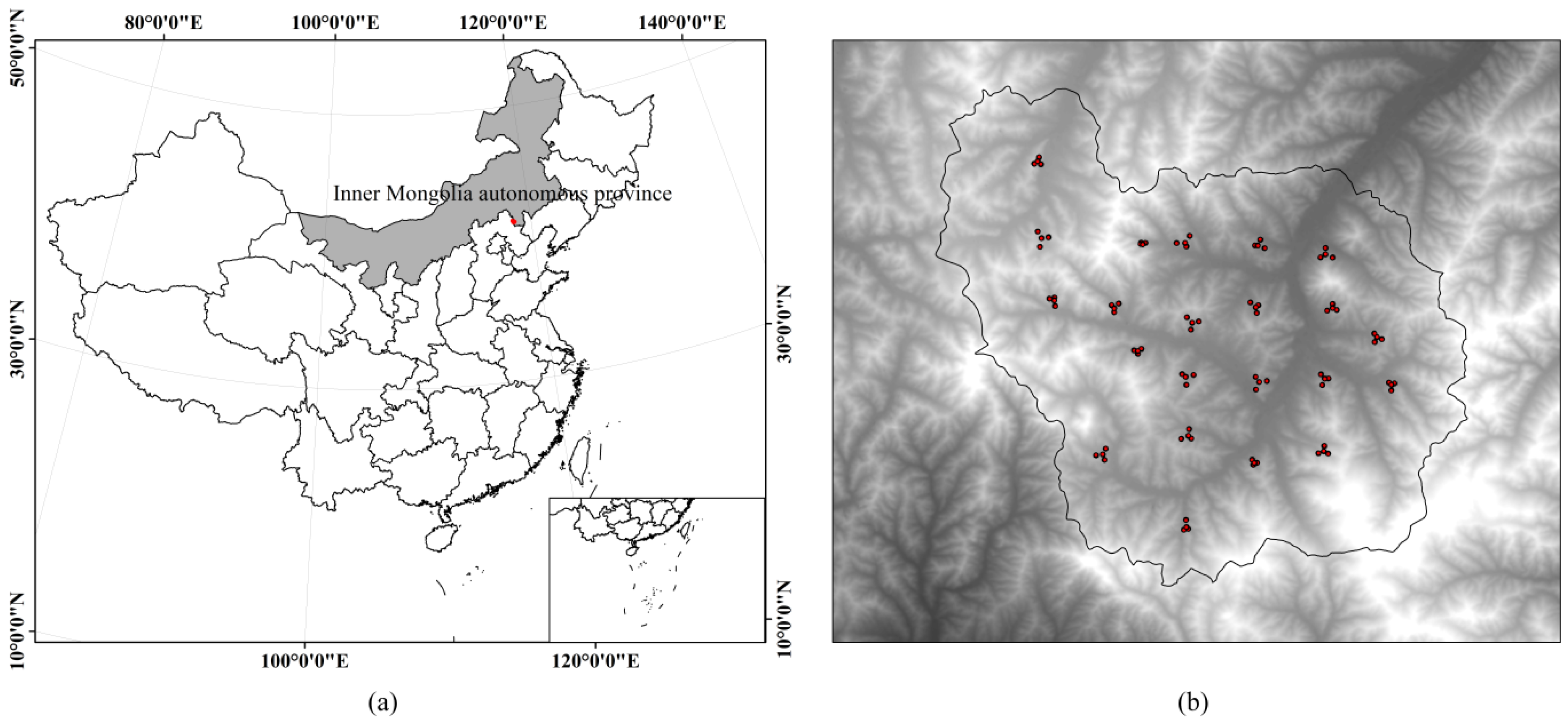
2.1. Study Site
2.2. Field Data
2.3. ULS and USP Datasets
2.4. Data Pre-Processing
2.4.1. Dense Point Clouds Generation from Images
2.4.2. Point Cloud Normalization and CHM Generation
2.4.3. Feature Metrics Generation
2.5. Data Analysis
3. Results
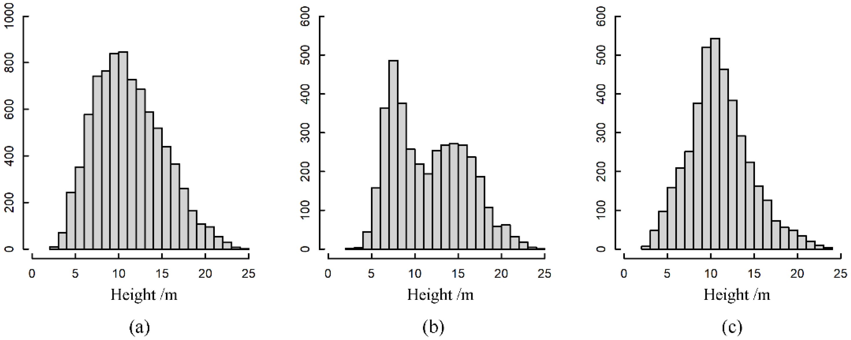
3.1. Visual Comparison of ULS Point Clouds and USP Point Clouds
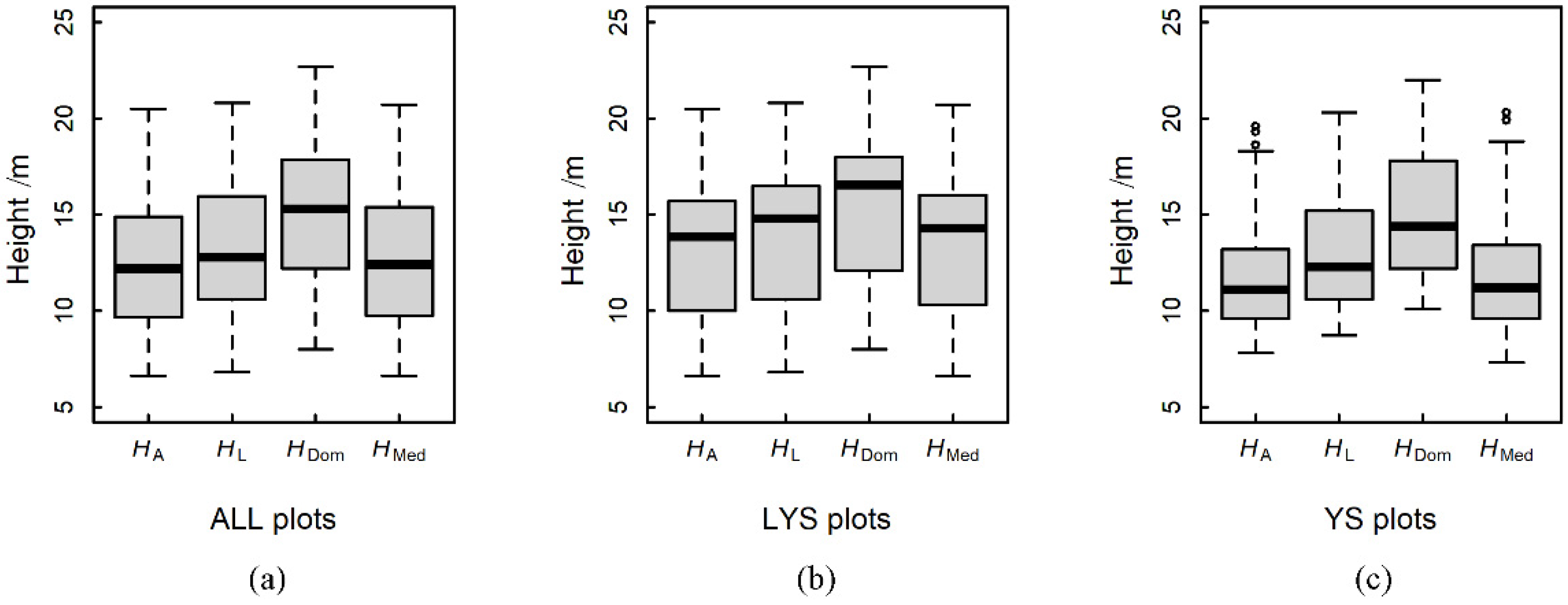
3.2. Forest Stand Heights Modeling Using ULS and USP Metrics
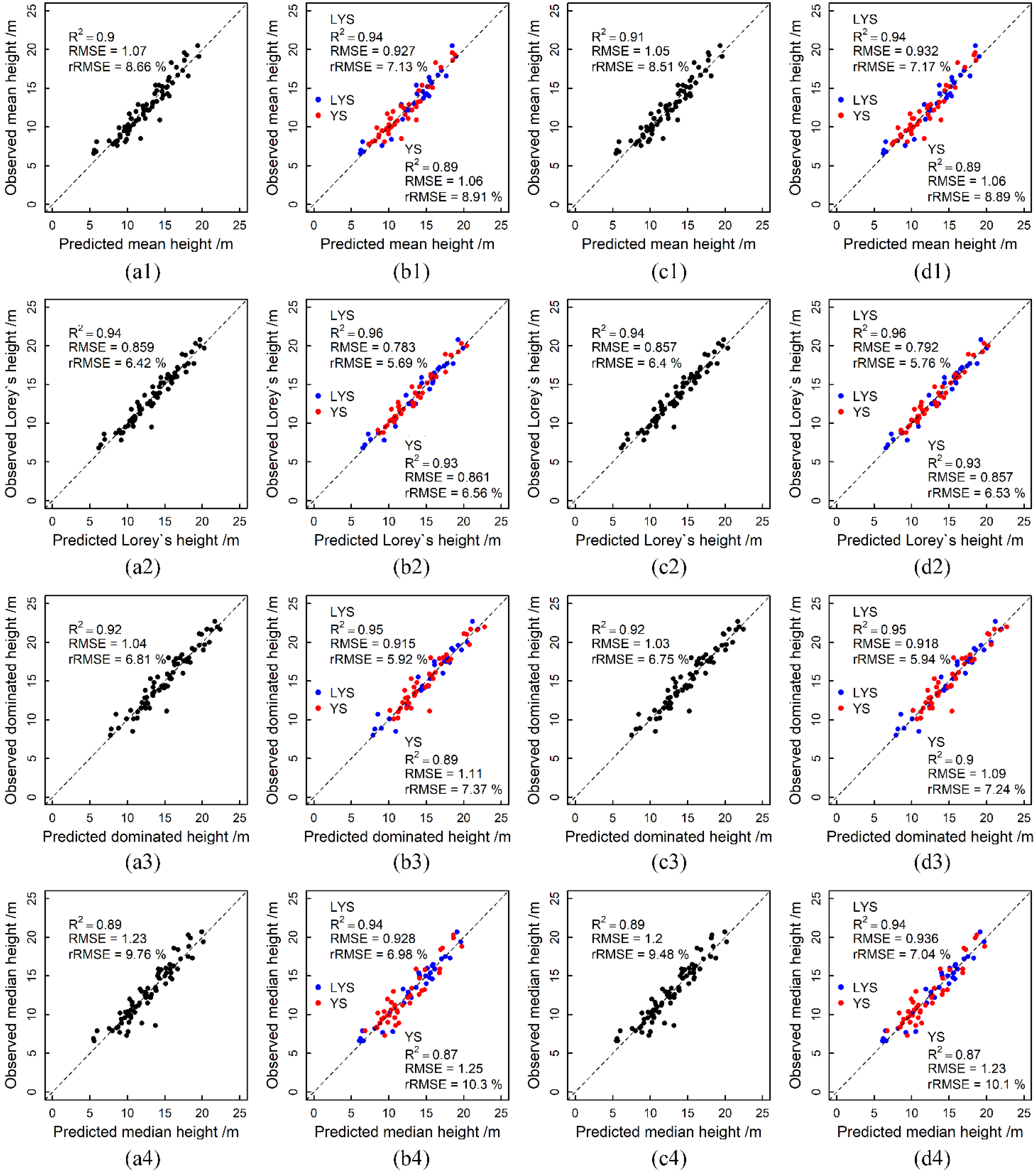
3.3. Forest Stand Height Estimation Accuracy
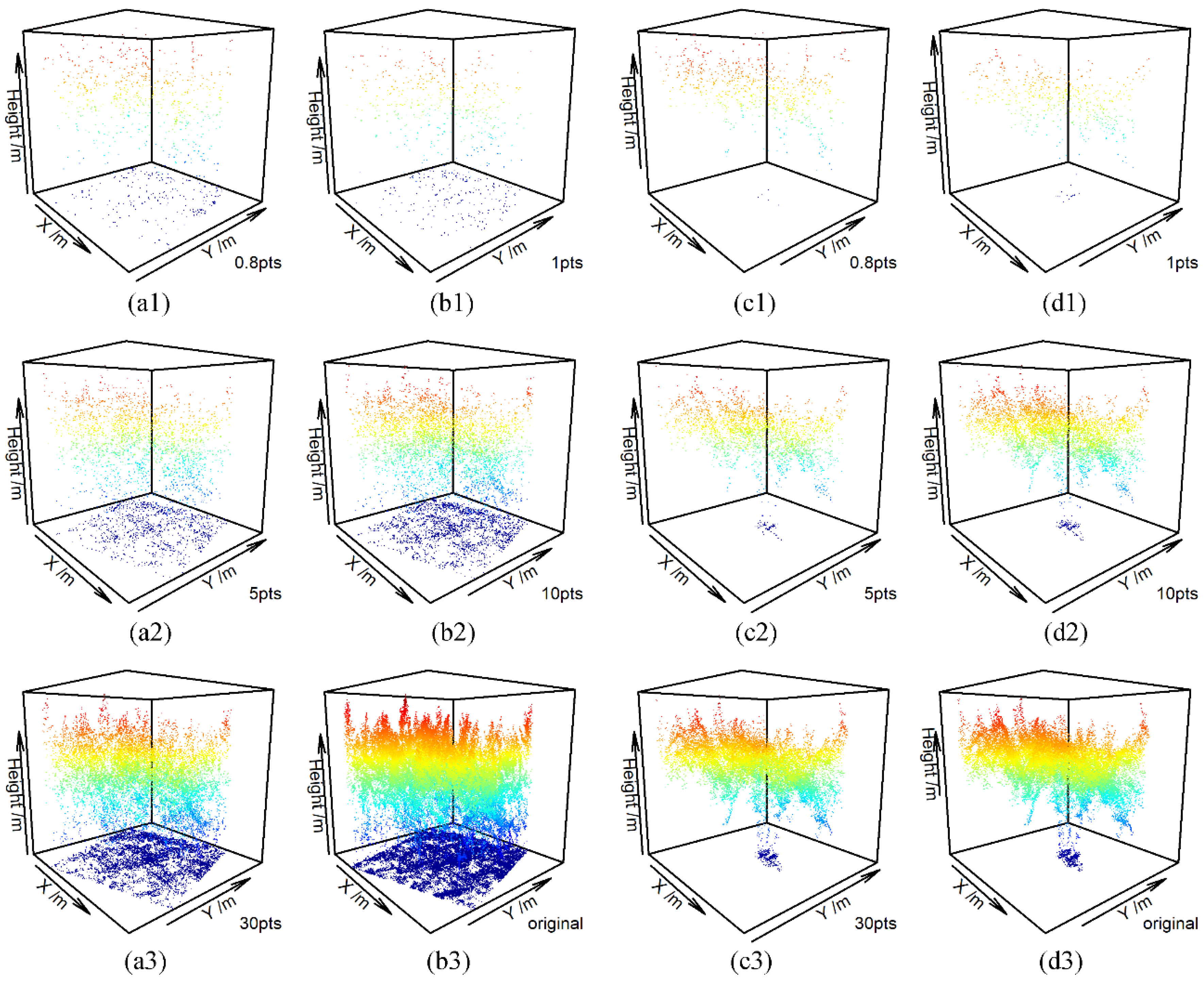
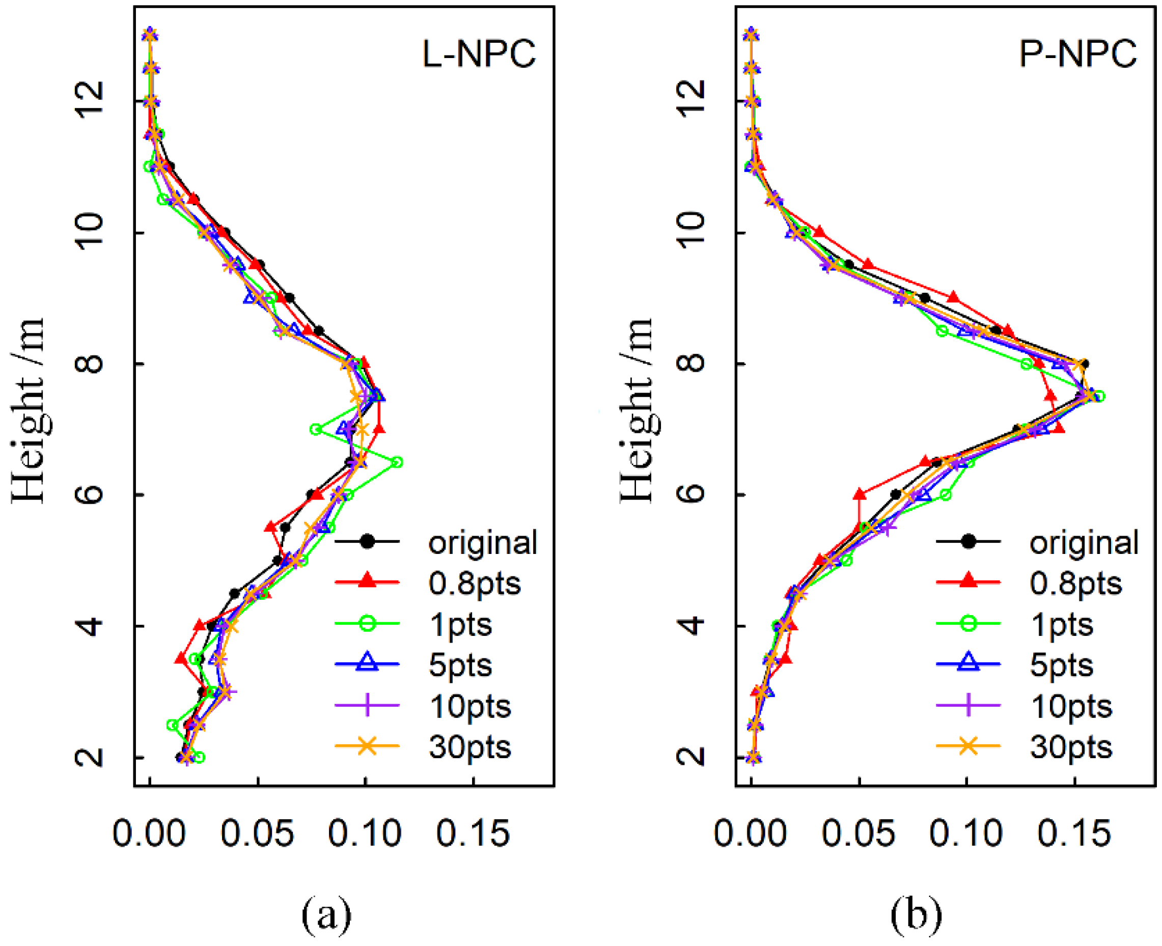
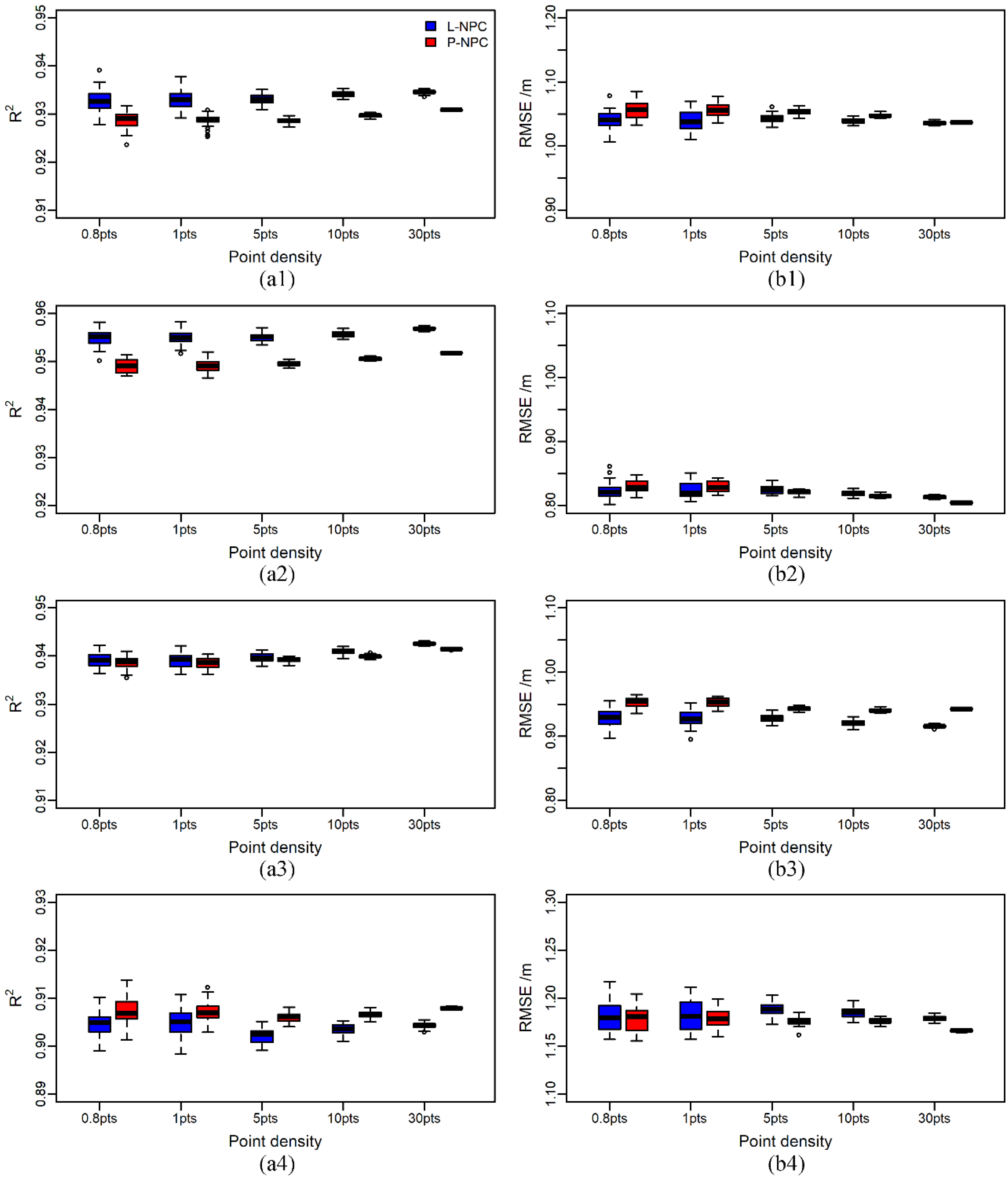
3.4. Estimation Results of Forest Stand Heights with Different Point Density
4. Discussion
4.1. The Capability of USP and ULS to Estimate Forest Stand Heights
4.2. The Best Explanatory Variables for Forest Stand Heights
4.3. The Influence of Point Density on the Estimation Accuracy
4.4. The Performances of Point Clouds and CHM
4.5. The Limitation of This Study
5. Conclusions
Author Contributions
Funding
Institutional Review Board Statement
Informed Consent Statement
Data Availability Statement
Acknowledgments
Conflicts of Interest
Nomenclature
| Acronyms | Full Name |
| UAV | Unmanned Aerial Vehicle |
| ULS | UAV Laser Scanning |
| USP | UAV Stereo Photogrammetry |
| DEM | Digital Elevation Model |
| DSM | Digital Surface Model |
| NPC | Normalized Point Clouds |
| L-NPC | NPC of LiDAR |
| P-NPC | NPC of USP |
| CHM | Canopy Height Model |
| L-CHM | CHM of ULS |
| P-CHM | CHM of USP |
| DBH | Diameter at Breast Height |
| HA | Mean height |
| HL | Lorey’s height |
| HDom | Dominated height |
| HMed | Median height |
Appendix A

| All Plots NPC Metrics | LYS Plots NPC Metrics | YS Plots NPC Metrics | All Plots CHM Metrics | LYS Plots CHM Metrics | YS Plots CHM Metrics | |||||||
|---|---|---|---|---|---|---|---|---|---|---|---|---|
| MD | r | MD | r | MD | r | MD | r | MD | r | MD | r | |
| h10 | −2.180 | 0.962 | −1.947 | 0.965 | −2.351 | 0.962 | −2.076 | 0.948 | −1.807 | 0.955 | −2.273 | 0.939 |
| h20 | −1.591 | 0.976 | −1.388 | 0.981 | −1.740 | 0.970 | −1.405 | 0.972 | −1.181 | 0.979 | −1.569 | 0.963 |
| h30 | −1.270 | 0.984 | −1.121 | 0.986 | −1.379 | 0.980 | −1.050 | 0.982 | −0.887 | 0.988 | −1.170 | 0.975 |
| h40 | −1.022 | 0.989 | −0.922 | 0.990 | −1.096 | 0.986 | −0.795 | 0.988 | −0.694 | 0.991 | −0.869 | 0.984 |
| h50 | −0.828 | 0.991 | −0.757 | 0.993 | −0.880 | 0.988 | −0.596 | 0.990 | −0.529 | 0.994 | −0.645 | 0.987 |
| h60 | −0.660 | 0.992 | −0.616 | 0.994 | −0.692 | 0.989 | −0.425 | 0.993 | −0.394 | 0.995 | −0.448 | 0.990 |
| h70 | −0.500 | 0.993 | −0.492 | 0.995 | −0.506 | 0.991 | −0.278 | 0.994 | −0.277 | 0.996 | −0.278 | 0.992 |
| h80 | −0.322 | 0.995 | −0.354 | 0.996 | −0.298 | 0.993 | −0.116 | 0.995 | −0.159 | 0.997 | −0.084 | 0.994 |
| h90 | −0.130 | 0.995 | −0.184 | 0.996 | −0.090 | 0.993 | 0.051 | 0.995 | −0.007 | 0.997 | 0.093 | 0.994 |
| h95 | −0.009 | 0.995 | −0.074 | 0.996 | 0.039 | 0.993 | 0.150 | 0.996 | 0.090 | 0.997 | 0.194 | 0.994 |
| hmax | −0.012 | 0.977 | −0.014 | 0.970 | −0.011 | 0.986 | −0.004 | 0.977 | −0.008 | 0.971 | −0.002 | 0.985 |
| hmean | −1.030 | 0.990 | −0.959 | 0.991 | −1.081 | 0.989 | −0.842 | 0.988 | −0.766 | 0.990 | −0.898 | 0.987 |
| hmed | −0.828 | 0.991 | −0.757 | 0.993 | −0.880 | 0.988 | −0.596 | 0.990 | −0.529 | 0.994 | −0.645 | 0.987 |
| hcv | 0.096 | 0.848 | 0.087 | 0.832 | 0.103 | 0.863 | 0.093 | 0.797 | 0.081 | 0.793 | 0.102 | 0.797 |
| hsd | 0.869 | 0.834 | 0.818 | 0.640 | 0.907 | 0.885 | 0.901 | 0.807 | 0.831 | 0.632 | 0.951 | 0.864 |
| hIQ | 1.002 | 0.859 | 0.816 | 0.629 | 1.139 | 0.889 | 1.013 | 0.861 | 0.794 | 0.709 | 1.174 | 0.887 |
| Height | L-NPC Metrics | L-CHM Metrics | P-NPC Metrics | P-CHM Metrics | ||||||||
|---|---|---|---|---|---|---|---|---|---|---|---|---|
| ALL | LYS | YS | ALL | LYS | YS | ALL | LYS | YS | ALL | LYS | YS | |
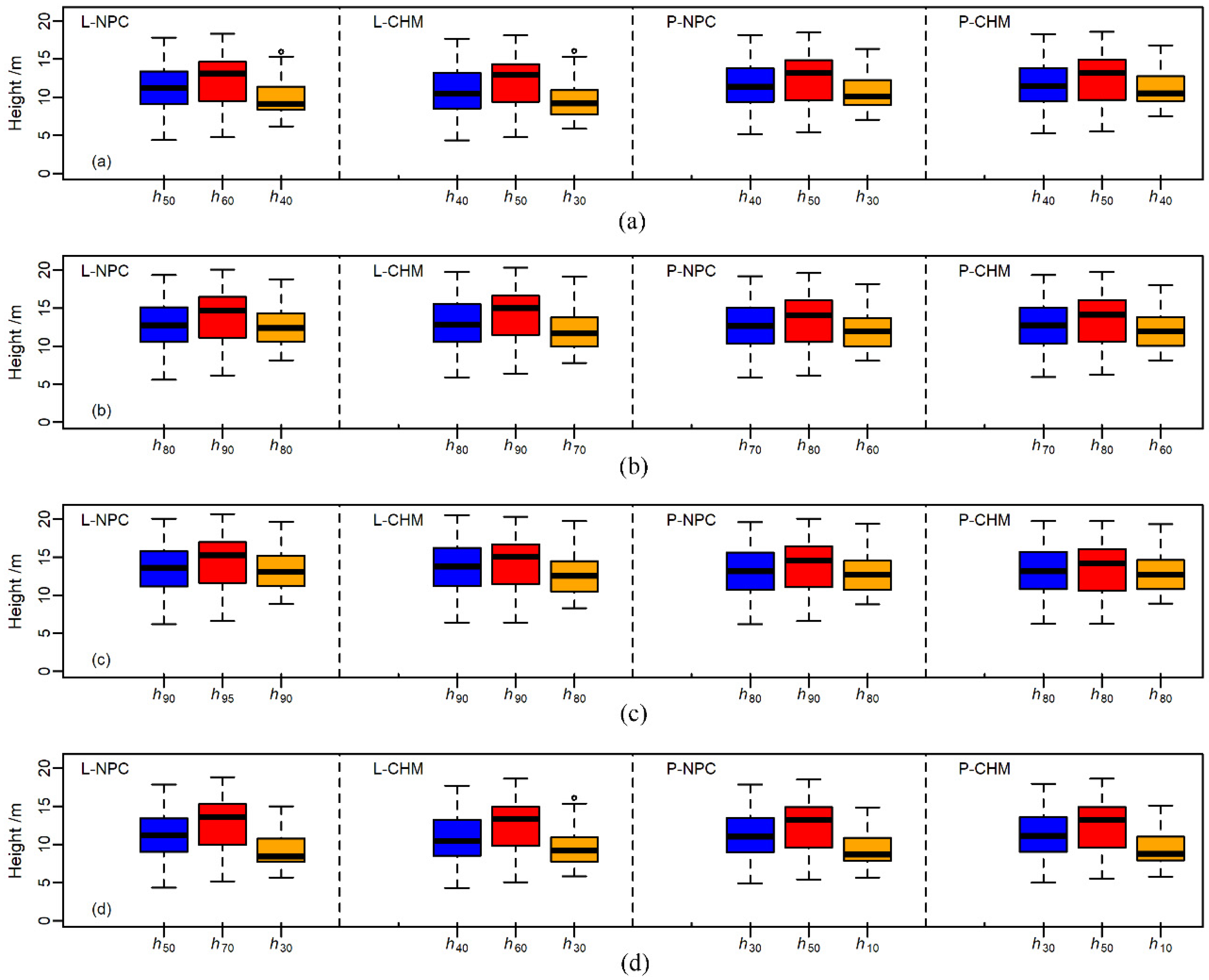
| HA | h50 | h60 | h40 | h40 | h50 | h30 | h40 | h50 | h30 | h40 | h50 | h40 |
| a = 0.859 | a = 1.667 | a = −0.564 | a = 0.971 | a = 1.418 | a = 0.256 | a = 0.108 | a = 1.003 | a = −1.377 | a = 0.005 | a = 0.949 | a = −1.696 | |
| b = 1.037 | b = 0.936 | b = 1.237 | b = 1.054 | b = 0.971 | b = 1.210 | b = 1.061 | b = 0.967 | b = 1.237 | b = 1.065 | b = 0.968 | b = 1.211 | |
| HL | h80 | h90 | h80 | h80 | h90 | h70 | h70 | h80 | h60 | h70 | h80 | h60 |
| a = 0.339 | a = 0.506 | a = −0.655 | a = 0.073 | a = −0.025 | a = −0.076 | a = 0.053 | a = 0.489 | a = −0.834 | a = −0.022 | a = 0.449 | a = −0.981 | |
| b = 1.019 | b = 0.961 | b = 1.093 | b = 1.018 | b = 0.981 | b = 1.079 | b = 1.050 | b = 0.987 | b = 1.160 | b = 1.051 | b = 0.985 | b = 1.168 | |
| HDom | h90 | h95 | h90 | h90 | h90 | h80 | h80 | h90 | h80 | h80 | h80 | h80 |
| a = 0.898 | a = 1.057 | a = 0.051 | a = 0.611 | a = 0.975 | a = 0.764 | a = 0.975 | a = 1.070 | a = 0.071 | a = 0.889 | a = 1.490 | a = −0.081 | |
| b = 1.056 | b = 1.005 | b = 1.121 | b = 1.057 | b = 1.030 | b = 1.113 | b = 1.087 | b = 1.029 | b = 1.165 | b = 1.087 | b = 1.033 | b = 1.171 | |
| HMed | h50 | h70 | h30 | h40 | h60 | h30 | h30 | h50 | h10 | h30 | h50 | h10 |
| a = 0.618 | a = 0.980 | a = −0.565 | a = 0.740 | a = 0.751 | a = −0.062 | a = 0.139 | a = 0.673 | a = −1.005 | a = 0.025 | a = 0.619 | a = −1.005 | |
| b = 1.082 | b = 0.980 | b = 1.358 | b = 1.100 | b = 1.013 | b = 1.269 | b = 1.120 | b = 1.017 | b = 1.388 | b = 1.126 | b = 1.018 | b = 1.376 | |
References
- Food and Agriculture Organization of the United Nations (FAO). Global Forest Resources Assessment 2015: How Are the World’s Forests Changing? FAO: Rome, Italy, 2015; pp. 1–48. Available online: https://www.uncclearn.org/wp-content/uploads/library/a-i4793e.pdf (accessed on 20 May 2021).
- Jim, C.; Peter, H. Wood From Planted Forests: A Global Outlook 2005–2030. Acta Phytoecol. Sin. 2008, 28, 210–217. [Google Scholar]
- Pawson, S.M.; Brin, A.; Brockerhoff, E.G.; Lamb, D.; Payn, T.W.; Paquette, A.; Parrotta, J.A. Plantation forests, climate change and biodiversity. Biodivers. Conserv. 2013, 22, 1203–1227. [Google Scholar] [CrossRef]
- Liu, K.; Shen, X.; Cao, L.; Wang, G.; Cao, F. Estimating forest structural attributes using UAV-LiDAR data in Ginkgo plantations. ISPRS J. Photogramm. Remote Sens. 2018, 146, 465–482. [Google Scholar] [CrossRef]
- Dash, J.P.; Marshall, H.M.; Brian, R. Methods for estimating multivariate stand yields and errors using k-NN and aerial laser scanning. For. Int. J. For. Res. 2015, 88, 237–247. [Google Scholar] [CrossRef]
- Selkowitz, D.J.; Green, G.; Peterson, B.; Wylie, B. A multi-sensor lidar, multi-spectral and multi-angular approach for mapping canopy height in boreal forest regions. Remote Sens. Environ. 2012, 121, 458–471. [Google Scholar] [CrossRef]
- Zarco-Tejada, P.J.; Diaz-Varela, R.; Angileri, V.; Loudjani, P. Tree height quantification using very high resolution imagery acquired from an unmanned aerial vehicle (UAV) and automatic 3D photo-reconstruction methods. Eur. J. Agron. 2014, 55, 89–99. [Google Scholar] [CrossRef]
- Okojie, J. Assessment of Forest Tree Structural Parameter Extractability from Optical Imaging UAV Datasets, in Ahaus Germany. Master’s Thesis, University of Twente, Enschede, The Netherlands, 2017. [Google Scholar]
- Kankare, V.; Holopainen, M.; Vastaranta, M.; Puttonen, E.; Yu, X.; Hyyppae, J.; Vaaja, M.; Hyyppae, H.; Alho, P. Individual tree biomass estimation using terrestrial laser scanning. ISPRS J. Photogramm. Remote Sens. 2013, 75, 64–75. [Google Scholar] [CrossRef]
- Okojie, J.A.; Okojie, L.O.; Effiom, A.E.; Odia, B.E. Relative canopy height modelling precision from UAV and ALS datasets for forest tree height estimation. Remote. Sens. Appl. Soc. Environ. 2020, 17, 100284. [Google Scholar] [CrossRef]
- Lim, K.; Treitz, P.; Wulder, M.; St-Onge, B.T.; Flood, M. LiDAR remote sensing of forest structure. Prog. Phys. Geog. 2003, 27, 88–106. [Google Scholar] [CrossRef] [Green Version]
- Puliti, S.; Ørka, H.; Gobakken, T.; Næsset, E. Inventory of Small Forest Areas Using an Unmanned Aerial System. Remote Sens. 2015, 7, 9632–9654. [Google Scholar] [CrossRef] [Green Version]
- Puliti, S.; Saarela, S.; Gobakken, T.; Ståhl, G.; Næsset, E. Combining UAV and Sentinel-2 auxiliary data for forest growing stock volume estimation through hierarchical model-based inference. Remote Sens. Environ. 2018, 204, 485–497. [Google Scholar] [CrossRef]
- Maltamo, M.; Næsset, E.; Vauhkonen, J. Forestry Applications of Airborne Laser Scanning: Concepts and Case Studies. Manag. Ecosys. 2014, 27, 2014. [Google Scholar]
- Jonas, B.; Jrgen, W.; Franssonsupa, J.E.S. Forest variable estimation using photogrammetric matching of digital aerial images in combination with a high-resolution DEM. Scand. J. Forest Res. 2012, 27, 692–699. [Google Scholar]
- Iqbal, I.A.; Musk, R.A.; Osborn, J.; Stone, C.; Lucieer, A. A comparison of area-based forest attributes derived from airborne laser scanner, small-format and medium-format digital aerial photography. Int. J. Appl. Earth Obs. 2019, 76, 231–241. [Google Scholar] [CrossRef]
- Antonio Navarro, J.; Fernandez-Landa, A.; Luis Tome, J.; Luz Guillen-Climent, M.; Carlos Ojeda, J. Testing the quality of forest variable estimation using dense image matching: A comparison with airborne laser scanning in a Mediterranean pine forest. Int. J. Remote Sens. 2018, 39, 1–17. [Google Scholar]
- White, J.; Stepper, C.; Tompalski, P.; Coops, N.; Wulder, M. Comparing ALS and Image-Based Point Cloud Metrics and Modelled Forest Inventory Attributes in a Complex Coastal Forest Environment. Forests 2015, 6, 3704–3732. [Google Scholar] [CrossRef]
- Cao, L.; Liu, H.; Fu, X.; Zhang, Z.; Ruan, H. Comparison of UAV LiDAR and Digital Aerial Photogrammetry Point Clouds for Estimating Forest Structural Attributes in Subtropical Planted Forests. Forests 2019, 10, 145. [Google Scholar] [CrossRef] [Green Version]
- Noordermeer, L.; Bollandsås, O.M.; Ørka, H.O.; Næsset, E.; Gobakken, T. Comparing the accuracies of forest attributes predicted from airborne laser scanning and digital aerial photogrammetry in operational forest inventories. Remote Sens. Environ. 2019, 226, 26–37. [Google Scholar] [CrossRef]
- Ullah, S.; Adler, P.; Dees, M.; Datta, P.; Weinacker, H.; Koch, B. Comparing image-based point clouds and airborne laser scanning data for estimating forest heights. Iforest Biogeosci. For. 2017, 10, 273–280. [Google Scholar] [CrossRef] [Green Version]
- Mielcarek, M.; Kamińska, A.; Stereńczak, K. Digital Aerial Photogrammetry (DAP) and Airborne Laser Scanning (ALS) as Sources of Information about Tree Height: Comparisons of the Accuracy of Remote Sensing Methods for Tree Height Estimation. Remote Sens. 2020, 12, 1808. [Google Scholar] [CrossRef]
- Vastaranta, M.; Wulder, M.A.; White, J.C.; Pekkarinen, A.; Tuominen, S.; Ginzler, C.; Kankare, V.; Holopainen, M.; Hyyppä, J.; Hyyppä, H. Airborne laser scanning and digital stereo imagery measures of forest structure: Comparative results and implications to forest mapping and inventory update. Can. J. Remote Sens. 2013, 39, 382–395. [Google Scholar] [CrossRef]
- Lennart, N.; Martin, B.S.O.; Terje, G.; Erik, N.S. Direct and indirect site index determination for Norway spruce and Scots pine using bitemporal airborne laser scanner data. For. Ecol. Manag. 2018, 428, 104–114. [Google Scholar] [CrossRef]
- Zhao, K.; Suarez, J.C.; Garcia, M.; Hu, T.; Wang, C.; Londo, A. Utility of multitemporal lidar for forest and carbon monitoring: Tree growth, biomass dynamics, and carbon flux. Remote Sens. Environ. 2017, 204, 883–897. [Google Scholar] [CrossRef]
- Gleason, C.J.; Im, J. Forest biomass estimation from airborne LiDAR data using machine learning approoaches. Remote Sens. Environ. 2012, 125, 80–91. [Google Scholar] [CrossRef]
- Järnstedt, J.; Pekkarinen, A.; Tuominen, S.; Ginzler, C.; Holopainen, M.; Viitala, R. Forest variable estimation using a high-resolution digital surface model. ISPRS J. Photogramm. Remote Sens. 2012, 74, 78–84. [Google Scholar] [CrossRef]
- Jensen, J.L.R.; Mathews, A.J. Assessment of Image-Based Point Cloud Products to Generate a Bare Earth Surface and Estimate Canopy Heights in a Woodland Ecosystem. Remote Sens. 2016, 8, 50. [Google Scholar] [CrossRef] [Green Version]
- Tompalski, P.; White, J.C.; Coops, N.C.; Wulder, M.A. Quantifying the contribution of spectral metrics derived from digital aerial photogrammetry to area-based models of forest inventory attributes. Remote. Sens. Environ. 2019, 234, 111434. [Google Scholar] [CrossRef]
- Ruiz, L.; Hermosilla, T.; Mauro, F.; Godino, M. Analysis of the Influence of Plot Size and LiDAR Density on Forest Structure Attribute Estimates. Forests 2014, 5, 936–951. [Google Scholar] [CrossRef] [Green Version]
- Lovell, J.L.; Jupp, D.L.B.; Newnham, G.J.; Coops, N.C.; Culvenor, D.S. Simulation study for finding optimal lidar acquisition parameters for forest height retrieval. For. Ecol. Manag. 2005, 214, 398–412. [Google Scholar] [CrossRef]
- Mattias, M.; Fransson, J.E.S.; Johan, H. Effects on estimation accuracy of forest variables using different pulse density of laser data. For. Sci. 2007, 53, 619–626. [Google Scholar]
- Garcia, M.; Saatchi, S.; Ferraz, A.; Silva, C.A.; Ustin, S.; Koltunov, A.; Balzter, H. Impact of data model and point density on aboveground forest biomass estimation from airborne LiDAR. Carbon Balance Manag. 2017, 12, 1–18. [Google Scholar] [CrossRef] [Green Version]
- Popescu, S.C.; Wynne, R.H.; Nelson, R.F. Estimating plot-level tree heights with lidar: Local filtering with a canopy-height based variable window size. Comput. Electron. Agr. 2002, 37, 71–95. [Google Scholar] [CrossRef]
- Verhoeven, G. Taking computer vision aloft–archaeological three-dimensional reconstructions from aerial photographs with photoscan. Archaeol. Prospect. 2011, 18, 67–73. [Google Scholar] [CrossRef]
- Liu, Q.W.; Fu, L.; Chen, Q.; Wang, G.X.; Luo, P.; Sharma, R.P.; He, P.; Li, M.; Wang, M.X.; Duan, G.S. Analysis of the Spatial Differences in Canopy Height Models from UAV LiDAR and Photogrammetry. Remote Sens. 2020, 12, 2884. [Google Scholar] [CrossRef]
- Wu, B.; Tang, S.J. Review of geometric fusion of remote sensing imagery and laser scanning data. Int. J. Image Data Fusion 2015, 6, 1–18. [Google Scholar] [CrossRef]
- Ni, W.J.; Sun, G.Q.; Pang, Y.; Zhang, Z.Y.; Liu, J.L.; Yang, A.Q.; Wang, Y.; Zhang, D.F. Mapping Three-Dimensional Structures of Forest Canopy Using UAV Stereo Imagery: Evaluating Impacts of Forward Overlaps and Image Resolutions with LiDAR Data as Reference. IEEE J. Sel. Top. Appl. Earth Obs. Remote. Sens. 2018, 11, 3578–3589. [Google Scholar] [CrossRef]
- Pyrl, J.; Saarinen, N.; Kankare, V.; Coops, N.C.; Vastaranta, M. Variability of wood properties using airborne and terrestrial laser scanning. Remote Sens. Environ. 2019, 235, 111474. [Google Scholar]
- Mcgaughey, R.J. FUSION/LDV: Software for LIDAR Data Analysis and Visualization; Pacific Northwest Research Station; University of Washington: Seattle, WA, USA, 2013. [Google Scholar]
- Næsset, E. Predicting forest stand characteristics with airborne scanning laser using a practical two-stage procedure and field data. Remote Sens. Environ. 2002, 80, 88–99. [Google Scholar] [CrossRef]
- Bottalico, F.; Chirici, G.; Giannini, R.; Mele, S.; Mura, M.; Puxeddu, M.; Mcroberts, R.E.; Valbuena, R.; Travaglini, D. Modeling Mediterranean forest structure using airborne laser scanning data. Int. J. Appl. Earth Obs. 2017, 57, 145–153. [Google Scholar] [CrossRef]
- Gobakken, T.; Bollandsås, O.M.; Næsset, E. Comparing biophysical forest characteristics estimated from photogrammetric matching of aerial images and airborne laser scanning data. Scand. J. For. Res. 2015, 30, 73–86. [Google Scholar] [CrossRef]
- Silva, C.A.; Hudak, A.; Vierling, L.A.; Klauberg, C.; Garcia, M.; Ferraz, A.; Keller, M.; Eitel, J.; Saatchi, S. Impacts of Airborne Lidar Pulse Density on Estimating Biomass Stocks and Changes in a Selectively Logged Tropical Forest. Remote Sens. 2017, 9, 1068. [Google Scholar] [CrossRef] [Green Version]
- Tesfamichael, S.G.; Aardt, J.A.N.V.; Ahmed, F. Estimating plot-level tree height and volume of Eucalyptus grandis plantations using small-footprint, discrete return lidar data. Prog. Phys. Geog. 2010, 34, 515–540. [Google Scholar] [CrossRef] [Green Version]
- Goldbergs, G.; Maier, S.; Levick, S.; Edwards, A. Efficiency of Individual Tree Detection Approaches Based on Light-Weight and Low-Cost UAS Imagery in Australian Savannas. Remote Sens. 2018, 10, 161. [Google Scholar] [CrossRef] [Green Version]
- Li, W.K.; Guo, Q.H.; Jakubowski, M.K.; Kelly, M. A New Method for Segmenting Individual Trees from the Lidar Point Cloud. Photogramm. Eng. Remote Sens. 2012, 78, 75–84. [Google Scholar] [CrossRef] [Green Version]
- Hirschmugl, M.; Ofner, M.; Raggam, J.; Schardt, M.S. Single tree detection in very high resolution remote sensing data. Remote Sens. Environ. 2007, 110, 533–544. [Google Scholar] [CrossRef]
- Li, Y.C.; Li, C.; Li, M.; Liu, Z. Influence of Variable Selection and Forest Type on Forest Aboveground Biomass Estimation Using Machine Learning Algorithms. Forests 2019, 10, 1073. [Google Scholar] [CrossRef] [Green Version]
- Racine, E.; Coops, N.C.; Bégin, J.; Myllymki, M. Species, crown closure, and age as determinants of the vertical distribution of airborne LiDAR returns. Trees 2021. [CrossRef]


| Forest Parameters | Symbol | Range | Median | Mean | SD |
|---|---|---|---|---|---|
| ALL plots (n = 71) | |||||
| Stand density/(stems ha−1) | N | 435–4097 | 1714 | 1728 | 695 |
| Mean DBH/cm | DBH | 7.70–31.20 | 14.00 | 15.18 | 4.73 |
| Canopy cover | CC | 0.42–0.87 | 0.63 | 0.63 | 0.09 |
| Lorey’s height/m | HL | 6.80–20.80 | 12.80 | 13.39 | 3.49 |
| Mean height/m | HA | 6.60–20.50 | 12.20 | 12.39 | 3.49 |
| Dominated height/m | HDom | 8.00–22.70 | 15.30 | 15.24 | 3.69 |
| Median height/m | HMed | 6.6–20.70 | 12.40 | 12.66 | 3.69 |
| Volume/(m3 ha−2) | V | 62.40–374.40 | 206.40 | 209.67 | 70.70 |
| LYS plots (n = 30) | |||||
| Stand density/(stems ha−1) | N | 528–4097 | 1794 | 1902 | 768 |
| Mean DBH/cm | DBH | 7.70–22.50 | 14.15 | 14.02 | 3.89 |
| Canopy cover | CC | 0.43–0.87 | 0.66 | 0.65 | 0.10 |
| Lorey’s height/m | HL | 6.80–20.80 | 14.80 | 13.76 | 3.85 |
| Mean height/m | HA | 6.60–20.50 | 13.85 | 13.00 | 3.77 |
| Dominated height/m | HDom | 8.00–22.70 | 16.55 | 15.45 | 4.06 |
| Median height/m | HMed | 6.60–22.70 | 14.30 | 13.29 | 3.96 |
| Volume/(m3 ha−2) | V | 62.40–374.40 | 220.00 | 208.27 | 83.45 |
| YS plots (n = 41) | |||||
| Stand density/(stems ha−1) | N | 435–2536 | 1674 | 1600 | 615 |
| Mean DBH/cm | DBH | 10.80–31.20 | 13.80 | 16.03 | 5.14 |
| Canopy cover | CC | 0.42–0.78 | 0.62 | 0.62 | 0.08 |
| Lorey’s height/m | HL | 8.70–20.30 | 12.30 | 13.12 | 3.22 |
| Mean height/m | HA | 7.80–19.60 | 11.10 | 11.94 | 3.24 |
| Dominated height/m | HDom | 10.10–22.00 | 14.40 | 15.09 | 3.44 |
| Median height/m | HMed | 7.30–20.30 | 11.20 | 12.19 | 3.45 |
| Volume/(m3 ha−2) | V | 108.80–372.80 | 206.4 | 210.69 | 60.80 |
| LiDAR | |||
|---|---|---|---|
| UAV model | RC6-2000 | Rotor | 8 |
| LiDAR model | Riegl VUX-1 | PRF | 10 Hz~200 Hz |
| Laser wavelength | 905 nm | Laser divergence | 3 mrad |
| Scan pattern | Rotate Mirror | Scan FOV | 30° × 360° |
| Echoes | 2 | Max Scan frequency | 20 Hz |
| Range | 3 m~−920 m | Vertical Accuracy | <5 cm |
| Photogrammetry | |||
| UAV model | DJI Phantom 4 RTK | Rotor | 3 |
| Camera model | 1 mm CMOS | Pixels | 50,320,896 |
| CMOS size | 36.0 mm × 24.0 mm | Image size | 4864 × 3648 pixels |
| FOV | Horizonal 70° Vertical ±10° | Focal length | 9 mm |
| Pixel unit | 4.1 µm × 4.1 µm | Bands | R/G/B |
| Category | Parameters | Describing |
|---|---|---|
| Height percentiles | h10, h20, …, h80, h90, h95 | Height percentile value for point clouds or CHM cells over 2 m |
| Height statistical metrics | hmax | Maximum value for point clouds or CHM cells over 2 m |
| hmean | Mean value for point clouds or CHM cells over 2 m | |
| hmed | Median value for point clouds or CHM cells over 2 m | |
| hcv | Coefficient of variation for point clouds or CHM cells over 2 m | |
| hsd | Standard deviation for point clouds or CHM cells over 2 m | |
| hIQ | h75 minus h25 | |
| Density statistical metrics | CRR | (hmean − hmin)/(hmax − hmin) |
| CC2m | Percentage of point cloud above 2 m | |
| CCmean | Percentage of point cloud above mean | |
| CCmode | Percentage of point cloud above mode |
| CC Level | CC | L-NPC | P-NPC | ||||
|---|---|---|---|---|---|---|---|
| pts/m2 | Minimum | Maximum | pts/m2 | Minimum | Maximum | ||
| High CC | 0.92 | 71 | 0 | 17.36 | 47 | 4.65 | 17.02 |
| Median CC | 0.75 | 97 | 0 | 13.21 | 46 | 0 | 13.00 |
| Low CC | 0.49 | 47 | 0 | 8.65 | 44 | 0 | 8.59 |
| Data Type | Stand Height | ALL Plots | LYS Plots | YS Plots | ||||||
|---|---|---|---|---|---|---|---|---|---|---|
| R2 | RMSE /m | rRMSE % | R2 | RMSE /m | rRMSE % | R2 | RMSE /m | rRMSE % | ||
| L-NPC | HA | 0.91 | 1.01 | 8.16 | 0.94 | 0.93 | 7.14 | 0.92 | 0.92 | 7.70 |
| HL | 0.94 | 0.82 | 6.14 | 0.96 | 0.78 | 5.66 | 0.94 | 0.79 | 6.03 | |
| HDom | 0.93 | 0.98 | 6.45 | 0.95 | 0.88 | 5.71 | 0.91 | 1.01 | 6.75 | |
| HMed | 0.89 | 1.21 | 9.53 | 0.91 | 0.98 | 7.39 | 0.89 | 1.12 | 9.20 | |
| L-CHM | HA | 0.93 | 0.90 | 7.27 | 0.94 | 0.91 | 6.98 | 0.92 | 0.88 | 7.40 |
| HL | 0.95 | 0.76 | 5.66 | 0.96 | 0.75 | 5.47 | 0.94 | 0.81 | 6.18 | |
| HDom | 0.94 | 0.93 | 6.08 | 0.96 | 0.82 | 5.33 | 0.91 | 0.99 | 6.58 | |
| HMed | 0.91 | 1.11 | 8.78 | 0.93 | 1.04 | 7.79 | 0.84 | 1.38 | 11.3 | |
| P-NPC | HA | 0.91 | 1.04 | 8.37 | 0.94 | 0.87 | 6.71 | 0.9 | 1.02 | 8.56 |
| HL | 0.94 | 0.83 | 6.23 | 0.96 | 0.74 | 5.36 | 0.93 | 0.84 | 6.39 | |
| HDom | 0.92 | 1.01 | 6.63 | 0.95 | 0.85 | 5.53 | 0.90 | 1.07 | 7.08 | |
| HMed | 0.89 | 1.21 | 9.55 | 0.95 | 0.88 | 6.62 | 0.88 | 1.2 | 9.86 | |
| P-CHM | HA | 0.91 | 1.02 | 8.23 | 0.94 | 0.88 | 6.75 | 0.89 | 1.07 | 8.98 |
| HL | 0.94 | 0.83 | 6.22 | 0.96 | 0.76 | 5.56 | 0.93 | 0.86 | 6.54 | |
| HDom | 0.92 | 1.01 | 6.60 | 0.95 | 0.85 | 5.51 | 0.90 | 1.05 | 6.98 | |
| HMed | 0.90 | 1.18 | 9.36 | 0.93 | 1.03 | 7.78 | 0.83 | 1.42 | 11.64 | |
Publisher’s Note: MDPI stays neutral with regard to jurisdictional claims in published maps and institutional affiliations. |
© 2021 by the authors. Licensee MDPI, Basel, Switzerland. This article is an open access article distributed under the terms and conditions of the Creative Commons Attribution (CC BY) license (https://creativecommons.org/licenses/by/4.0/).
Share and Cite
Li, M.; Li, Z.; Liu, Q.; Chen, E. Comparison of Coniferous Plantation Heights Using Unmanned Aerial Vehicle (UAV) Laser Scanning and Stereo Photogrammetry. Remote Sens. 2021, 13, 2885. https://doi.org/10.3390/rs13152885
Li M, Li Z, Liu Q, Chen E. Comparison of Coniferous Plantation Heights Using Unmanned Aerial Vehicle (UAV) Laser Scanning and Stereo Photogrammetry. Remote Sensing. 2021; 13(15):2885. https://doi.org/10.3390/rs13152885
Chicago/Turabian StyleLi, Mei, Zengyuan Li, Qingwang Liu, and Erxue Chen. 2021. "Comparison of Coniferous Plantation Heights Using Unmanned Aerial Vehicle (UAV) Laser Scanning and Stereo Photogrammetry" Remote Sensing 13, no. 15: 2885. https://doi.org/10.3390/rs13152885
APA StyleLi, M., Li, Z., Liu, Q., & Chen, E. (2021). Comparison of Coniferous Plantation Heights Using Unmanned Aerial Vehicle (UAV) Laser Scanning and Stereo Photogrammetry. Remote Sensing, 13(15), 2885. https://doi.org/10.3390/rs13152885