Abstract
Atmospheric wind is an essential parameter in the global observing system. In this study, the water vapor field in Typhoon Lekima and its surrounding areas simulated by the Weather Research and Forecasting (WRF) model is utilized to track the atmospheric motion wind through the Farneback Optical Flow (OF) algorithm. A series of experiments are conducted to investigate the influence of temporal and spatial resolutions on the errors of tracked winds. It is shown that the wind accuracy from tracking the specific humidity is higher than that from tracking the relative humidity. For fast-evolving weather systems such as typhoons, the shorter time step allows for more accurate wind retrievals, whereas for slow to moderate evolving weather conditions, the longer time step is needed for smaller retrieval errors. Compared to the traditional atmospheric motion vectors (AMVs) algorithm, the Farneback OF wind algorithm achieves a pixel-wise feature tracking and obtains a higher spatial resolution of wind field. It also works well under some special circumstances such as very low water vapor content or the region where the wind direction is parallel to the moisture gradient direction. This study has some significant implications for the configuration of satellite microwave sounding missions through their derived water vapor fields. The required temporal and spatial resolutions in the OF algorithm critically determine the satellite revisiting time and the field of view size. The brightness temperature (BT) simulated through Community Radiative Transfer Model (CRTM) is also used to track winds. It is shown that the error of tracking BT is generally larger than that of tracking water vapor. This increased error may result from the uncertainty in simulations of brightness temperatures at 183 GHz.
1. Introduction
The fast and accurate global 3D wind field measurements are required for improving the global forecasting as well as for utilizing wind energy and achieving sustainable energy supply [1,2]. Today, it is difficult to obtain the wind data in polar regions, over vast oceans, and on high elevations [3,4]. Therefore, satellite wind measurement technology is widely explored to obtain the global wind field.
Currently, two types of satellite technologies are explored for atmospheric wind measurements. The active sensors such as scatterometers are well-developed for obtaining the ocean surface wind field and the Atmospheric Laser Doppler Instrument (ALADIN) onboard the Aeolus mission provides the horizontal wind components at sub-satellite points [5,6,7]. The atmospheric motion vector (AMV) can also be derived through tracking the movement of cloud or water vapor in sequences of satellite images and calculating the direction and distance of movement. The AMV technology has provided the upper-air wind observations and filled the gaps in the observation field [8]. In the past, many studies were made to assimilate the AMVs into numerical weather prediction (NWP) models and show a positive impact on the weather forecasts [3,9,10,11,12].
The AMV algorithm mainly consists of two steps: cloud or water vapor feature tracking and wind vector height assignment. For the feature-tracking algorithms, Fujita et al. [13] first artificially determined the movement of clouds on the visible images, which was inefficient and less accurate. Endlich et al. [14] used computer recognition technology to calculate the motion by calculating the brightness center according to the cloud area and brightness, which was similar to the gravity center in mechanics. Leese et al. [15] determined the cross-correlation coefficients to obtain the wind field according to the principle of fast Fourier transform, and then many studies were made to improve this method [16,17,18]. AMVs are required to have a height information [19]. The uncertainty of height assignment has been proven to be one of the largest error sources that restricts the assimilation of AMVs into NWP [20]. To solve this problem, Santek et al. [21] proposed using water vapor fields retrieved from satellite radiance data to track wind fields. Since the one-dimensional variation algorithm (1DVAR) accurately assigns the water vapor height [22], calculating AMVs from these water vapor profiles can avoid the height assigned uncertainty.
The quality of the retrieved water vapor profiles greatly influences AMVs’ accuracy. Since visible or infrared instruments could not provide information under cloud conditions, the water vapor profiles retrieved from such wavebands can only be used to obtain the wind fields under clear sky conditions [21]. The microwave sounding from satellites can penetrate into clouds and precipitation conditions, and the data can be used to directly monitor the vertical structure of atmospheric temperature and water vapor of the active weather systems such as typhoons [12,23]. The atmospheric 3D water vapor fields are retrieved from microwave sounders under different observation scenarios and possess spatial continuity and vertical consistency [24], making it possible to obtain all-sky 3D wind fields. However, the current microwave sounders are mainly carried onboard polar-orbiting satellites, and a constellation of these polar-orbiting satellites or a geostationary microwave sounding technology is required to obtain better wind field measurements [25,26]. However, it remains to be discussed how the spatial–temporal resolution of water vapor retrieved from microwave instruments affects the accuracy of AMVs. Understanding the relationship between them contributes to improved AMV tracking algorithms and the design of future microwave instrument platforms. Lambrightsen et al. [27] and Posselt et al. [28] conducted AMVs experiments by tracking WRF Model water vapor features. However, the tracking algorithm they used is a traditional local area pattern matching method, which only calculates the regional average wind vectors [16], failing to meet the requirements of future high-resolution satellite observations [29]. Additionally, the traditional algorithms have high computational costs and large errors. In this study, the Farneback optical flow (OF) algorithm [30] is proposed to track the water vapor feature pixel by pixel and saves much calculation cost.
This study aims to obtain pixel-wise 3D wind fields by tracking features of 3D water vapor fields using the Farneback OF method. The wind field directly simulated by the WRF model can be regarded as the “truth”. The deviation between “WRF wind field” and “OF wind field” can be considered as the wind results’ “error”. Analyzing the error structure and sensitivity can verify the feasibility of obtaining 3D wind fields by tracking 3D water vapor retrieved from microwave observations and will help to explore the sensitivity and requirements of the Farneback OF wind track algorithm to the satellite revisiting time and sensor’s field-of-view (FOV) sizes. In Section 2, we introduce WRF simulated data and the Farneback OF wind track algorithm. In Section 3, the AMVs’ error structure and sensitivity are compared and analyzed for different weather systems. The conclusions and suggestions for future work are described in Section 4.
2. Materials and Methods
2.1. Nature Runs
The 3D water vapor calculated by the WRF model is used as the simulated microwave sounder retrieved data. The WRF simulation is run with a horizontal resolution of about 3 km and the 101 levels at a sigma coordinate. The model top level reaches 1 hPa, and all variables are interpolated onto 12 pressure levels from 975 to 100 hPa where the AMV are tracked. The WRF output is sampled every 5 min. The spatial resolution of the grid data can be simply regarded as the instrument FOV sizes. Adjusting the FOV sizes from 3 km (see Figure 1a) to 6, 12, 18, 24, and 30 km (Figure 1b) to examine its influence on the AMVs results. Here, we take a degradation from 3 to 12 km as an example. One piece of longitude/latitude grid data is taken from the center grid of its 5 × 5 neighbor grids. For the moisture data, we calculate the average data of the 5 × 5 points and assign the average data to the center grid to degrade the resolution. The remaining points of the 5 × 5 grids are abandoned. The time interval of 5 min can be used as the highest possible satellite revisiting time. The data with the different time intervals are used to explore the algorithm sensitivity and the requirements of satellite revisiting time. The simulation field covers 2500 × 2500 km, containing both fast-evolving weathers such as super typhoon and advection areas where water vapor flows vary smoothly. These simulated data can help us to understand whether the Farneback OF wind track algorithm is adapted to different weather systems. It also helps to explore how to adjust the algorithm parameters and change the water vapor spatial–temporal resolutions. The simulation time lasts from 12:00 on 8 August 2019 (UTC) to 12:00 on 10 August 2019 (UTC). The super typhoon Lekima in 2019 happened to be active during the simulation. We start our experiment at 12:00 on 8 August 2019 (UTC). At this time, Lekima has formed a double-eye wall structure, and its intensity in terms of convection and precipitation continue to increase. Table 1 illustrates the experiment design.
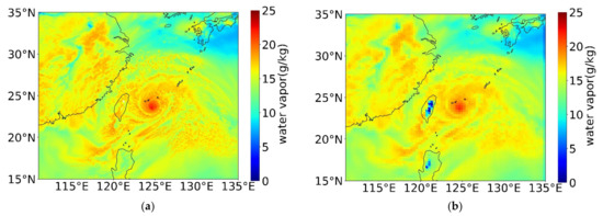
Figure 1.
Simulated water vapor field with different spatial resolution of 3 km (a) and 30 km (b) at 12:00 on 8 August 2019 (UTC) 850 hPa.

Table 1.
Wind track experiment design.
2.2. Simulated MWHS Brightness Temperature Data
To make our research more realistic, the WRF profiles data are used as input of the community radiative transfer model (CRTM version 2.4.0) to simulate the Microwave Humidity Sounder (MWHS) brightness temperature (BT). MWHS is carried on the FengYun-3D, launched on 14 December 2017. It has 15 channels, ranging from 89 to 183 GHz. Figure 2 shows the vertical distribution of weighting functions for MWHS channels. We choose BT at around 183 GHz water vapor absorption band as the tracer to derive winds. The weight function peak level of 183 GHz (shown in Table 2) is mainly at the middle-lower troposphere [22]. Here, we use the weighting function peak as the height of the wind vectors. To analyze the wind-tracking errors, we compare the BT wind fields with the WRF wind fields at the approximate layers. Figure 3 shows the BT of 183.31±7 GHz and the water vapor of 800 hPa. The approximate layers are also shown in Table 2. The purpose of this experiment is to confirm whether our OF wind-tracking algorithm is suitable for the wind retrieval based on MW observations and to compare the wind retrieve error difference between BT and water vapor fields.
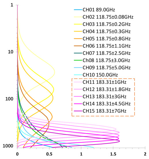
Figure 2.
The weighting functions for MWHS channels.
Table 2.
Water vapor channels information of MWHS.
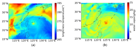
Figure 3.
The BT (a) of 183.31 ± 7 GHz and the water vapor (b) of 800 hPa.
2.3. Farneback OF Wind Track Algorithm
The core idea of the Farneback OF algorithm is to calculate the position of the same pixel at the next moment. It approximates the neighborhood of each pixel with a polynomial expansion expressed in a local coordinate system to accomplish image modeling. The polynomial expansion is shown as follows:
f(x) = xTAx + bTx + c
The dependent variable x represents the two-dimensional coordinate position (x y) T, A is a symmetric matrix, b a vector, and c a scalar. The coefficient A captures even part of the signal information except direct current (DC), b captures the odd part, and c varies with the local DC level [31]. According to the principle that coefficients can keep constant after a little motion, they are estimated by the weighted least squares method fit to the signal valued in the neighborhood [30].
The OF method must satisfy the assumption that the variation of the OF (the vector) is approximately smooth [32]. However, when it is applied to the wind track in the typhoon area, the assumption is not out of question due to the rapid changes of water vapor and the high-speed rotation around the typhoon eyewall area. The image pyramid method [33] is incorporated into the Farneback OF algorithm to solve this problem. Basically, the images at different scales are resized so that the algorithm can better capture the displacements at different scales. As shown in Figure 4, the pyramid bottom is of the original image size, and the image is resized 0.5 times its previous size upwards sequentially. The motion scale is also continuously resized so that the large-scale motion around the typhoon’s eyewall will be resized to meet the assumption which guarantees the effectiveness of the OF method.
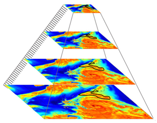
Figure 4.
Schematic diagram of image pyramid method with an original size at the bottom and the resizing rate of 0.5.
2.4. Quality Control Strategy
Quality control is critical in the AMVs algorithm. The pixels at the edge of image may move out of the area or the OF tracked by some pixels may be different from the overall tendency of the surroundings due to the limitations of the OF method. These situations need to be considered in the quality control process, which should follow the objective principles. The commonly used AMVs quality identifications are related to clouds [11,34], while our research is not restricted by clouds. Therefore, the following quality control schemes are proposed (Table 3). The wind vector that exceeds the simulated area is identified as 1. The wind vector of pixels with abnormal water vapor is identified as 2. The acceleration of u or v component exceeding 10 m/s2 indicates that the wind vector is inconsistent with the flow tendency, which belongs to the abnormal situation of OF identification, so it is identified as 3 or 4, respectively. If the two conditions are met at the same time, it is identified as 5. For the wind vector whose wind speed is too low (the threshold here is set to 0.5 m/s), we identify it as 6. Good quality wind vectors are identified as 0.
Table 3.
The quality control strategy.
3. Results and Discussion
3.1. AMVs Sensitivity to FOV Sizes at Various Heights
Here, we select four layers of 850, 500, 300, and 100 hPa for analysis as the experiment results indicate that AMVs sensitivity to the FOV sizes has obvious vertical characteristics. The WRF wind fields of 850, 500, 300, and 100 hPa are shown as Figure 5a,c,e,g, respectively. The OF wind fields of the selected four layers are shown as Figure 5b,d,f,h, respectively. The initial tracking time is 12:00 on 8 August 2019 (UTC), and the satellite revisiting time is set as 5 min.
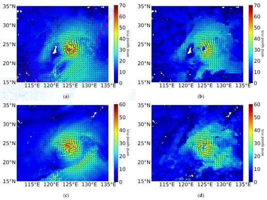
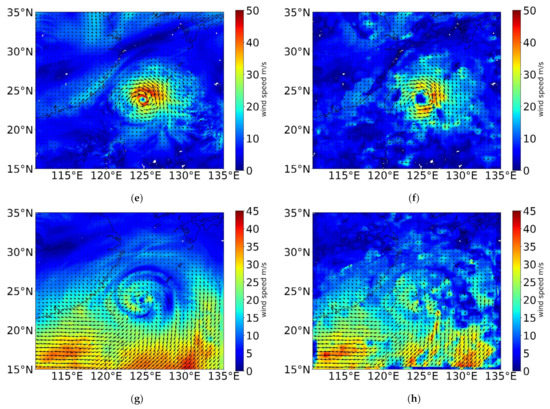
Figure 5.
The WRF wind fields and OF wind fields of 850 (a,b), 500 (c,d), 300 (e,f), and 100 hPa (g,h) on 12:05 on 8 August 2019 (UTC). The satellite revisiting time is set to 5 min. FOV size is set to 3 km.
To explore the relationship between the error and FOV sizes, we analyze the error of different layers with various FOV sizes and revisiting time. On every layer, the spatial resolution is adjusted from 3 to 6, 12, 18, 24, and 30 km. The resolution degradation method has been described in Section 2.1. We track wind of the data with a different spatial resolution (different FOV sizes) on every layer. Figure 6a,c,e,g show the wind speed relative error (RE) at 850, 500, 300, and 100 hPa, respectively. The wind speed RE is computed as
where the uWRF/vWRF represents the WRF wind, uOF/vOF represents the OF wind, and the N is the number of data points. Figure 6b,d,f,h show the root mean square error (RMSE) at four levels. The wind speed RMSE is computed as:
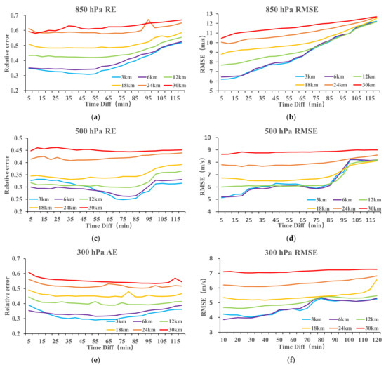
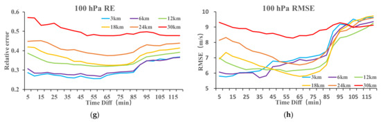
Figure 6.
The relative error (a,c,e,g) and the root mean square error (b,d,f,h) with different FOV sizes (shown as lines of different colors): 3, 6, 12, 18, 24, and 30 km. The X-axis represents satellite revisiting time ranging from 5 to 120 min in 5 min intervals.
The X-axis represents the satellite revisiting time ranging from 5 to 120 min, and the solid lines in different colors represent different FOV sizes. Results show that the error continues to reduce as the FOV sizes decrease, indicating that the error is sensitive to FOV sizes. We can conclude that increasing the satellite spatial resolution leads to higher accuracy wind fields. In addition, changing the spatial resolution will also affect the AMVs sensitivity to revisiting time. AMVs present more sensitivity to the revisiting time at small FOV sizes (Figure 6a,b,d,h). The RE and RMSE are irrelevant to the satellite revisiting time at large FOV sizes (18–30 km). It indicates that for the satellite data with low spatial resolution, it is hard to improve the wind-tracking accuracy even if the satellite revisiting time is shortened.
3.2. AMVs Sensitivity to Satellite Revisiting Time at Various Heights
To explore the AMVs sensitivity to the revisiting time and demonstrate the Farneback OF algorithm requirement for the satellite temporal resolution, we calculate the wind speed RE (Figure 7a), wind speed RMSE (Figure 7b), and wind direction absolute error (AE, see Figure 7c) of various satellite revisiting time at different heights. The wind direction AE is computed as:
where the dirWRF/dirOF is the wind direction of two wind fields. Due south is defined as 0° and 0–360° is defined as clockwise rotation. N is the number of data points. Note that in Figure 7, the X-axis represents time intervals, and solid lines in various colors represent 12 chosen heights. Figure 7a,c show that the upper and lower layers AMVs errors are more sensitive to the revisiting time than that of mid-layer. For the upper and lower layers, the wind speed RE(RMSE) increases significantly from nearly 30% (5–6 m/s) to 50% (12 m/s); meanwhile, the wind direction AE increases from 18° to 35° as the revisiting time extends from 30 to 120 min. While for the middle layers, the wind speed errors vary less from different revisiting times, and the wind direction error is negatively correlated with the satellite revisiting time, especially when the revisiting time is shorter than 30 min (Figure 7c). In addition, Figure 7a,b show a slight downward trend of the wind speed error at nearly all heights when the revisiting time is less than 30 min. Within a short revisiting time, the water vapor motion may be too smooth to be identified by the tracking model, especially at mid-layers where a tiny water vapor gradient or a slow motion exists. However, the high-speed rotating motion and severe changes in water vapor content at the typhoon center require a satellite data with a high time resolution. Therefore, the requirements for time resolution of Farneback OF wind-tracking algorithm under different weather systems need to be discussed.
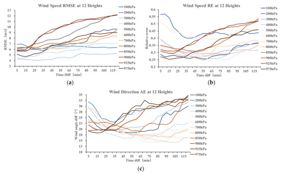
Figure 7.
The wind speed RE (a), wind speed RMSE (b), and wind direction AE (c) between WRF wind fields and Farneback OF wind fields of different satellite revisiting times at 12 heights.
3.3. Analysis of AMVs Error and Algorithm Requirements under Different Weather Systems
In order to analyze AMVs error under different weather conditions, we choose 400 hPa height wind field as an example, where the error decreases significantly with the revisiting time. As shown in Figure 7a,c, the wind speed RE and wind direction AE are 35.17% and 22.79°, respectively, while the revisiting time is set to 5 min. These errors are reduced to 25.37% and 16.05°, respectively, when the revisiting time extends to 50 min. Figure 8 depicts the WRF wind field (Figure 8a,c), the OF wind field (Figure 8b,d), and the relationship between them (Figure 8e,f). Comparing Figure 8b,d, the tracking effect in the typhoon’s central area is significantly more accurate than that of 50 min. The Beaufort wind force scale indicates that force 8 represents fresh gale in a cyclonic storm [35]. The scale 8 ranges in 17.5–20.5 m/s. Here, we assume the wind speed in 0–17.5 m/s mainly exists in the non-typhoon area and “>17.5 m/s” represents the typhoon area. Figure 8g,h show the wind-speed errors (AE and RE) in the non-typhoon area decreases and increases in the typhoon area, respectively. As the high-wind-speed range is mainly located in the typhoon area, where the water vapor stays strong and exhibits rotational movement under strong wind speed conditions, longer revisiting time will result in inaccurate displacement tracking due to the large difficulty of directly judging the large and rotating water vapor trajectory through two images.
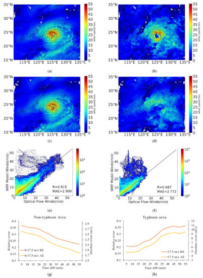
Figure 8.
WRF wind field at 400 hPa with the revisiting time of 5 min (a) and 50 min (c). Farneback wind field at 400 hPa with the revisiting time of 5 min (b) and 50 min (d). The background color shows the wind speed. Comparison of two wind fields with the revisiting time of 5 min (e) and 50 min (f). The X- and Y-axis of (e,f) represent OF and WRF wind speed, respectively. The wind speed RE (primary Y-axis) and AE (secondary Y-axis) of non-typhoon area (g) and typhoon area (h).
The typhoon area we choose to analyze covers 600 × 500 km, containing the fields of which the wind speed is greater than force 8 (Figure 9a). Figure 9 depicts the WRF wind field (a) and the OF wind field (b) in the center of the typhoon area at 400 hPa when the revisiting time is set to 5 min. The wind-tracking accuracy outside the typhoon eyewall is high, while it is poor in the eyewall area. As shown in Table 4, the wind speed RE and wind direction AE in the whole simulated area are 35.17% and 22.9°, respectively, while those error parameters in the typhoon area decrease to 15.31% and 7.67°, respectively. Combining with Figure 8b,d, we can conclude that the satellite revisiting time of the data used for fast-evolving and fast-changing weather systems wind tracking such as typhoons should be as short as possible.
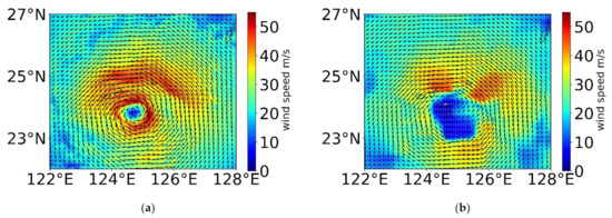
Figure 9.
WRF wind field (a) and OF wind field (b) at 400 hPa of the typhoon area with the 5 min revisiting time.
Table 4.
The wind-tracking errors of the whole simulated area and typhoon central area at 400 hPa, with revisiting time set to 5 min.
Figure 8g shows that the wind-tracking error of most non-typhoon areas decreases with the increase of revisiting time. To explore the factors affecting wind retrieval errors in the slowly evolving weather systems, we select an area with low water vapor content and relatively smooth water vapor movement, as shown in Figure 10. It covers 800 × 1000 km. Figure 10a–d, respectively, represent the WRF wind field and OF wind field of the selected smooth area at 400 hPa with 5 min (50 min) revisiting time. Comparing with 5 min revisiting time, the wind speed RE and the wind direction AE reduced by about 15.45% and 13.61°, respectively, when the revisiting time is set to 50 min (see Table 5). This error reduction is reasonable as the water vapor in this area moves slowly with a stable moving direction and small water vapor gradient. When the time interval is short, the difference between two water-vapor images is too smooth to be identified due to the very small displacement. The algorithm noise accounts for a large amount and the low signal-to-noise ratio leads to large errors. Therefore, for slow-evolving weather systems with smooth water vapor flow, tracking water vapor with longer time intervals can improve the accuracy of AMVs. It is concluded that the Farneback OF wind-tracking errors may be affected by many factors such as water vapor content, water vapor gradient, and wind speed [9].
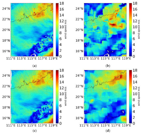
Figure 10.
The WRF wind field (a) and OF wind field (b) of the selected smooth area with 5 min revisiting time at 400 hPa. The WRF wind field (c) and OF wind field (d) of the selected smooth area with 50 min revisiting time at 400 hPa.
Table 5.
The wind-tracking errors of the selected smooth area at 400 hPa with 5 min and 50 min revisiting time.
3.4. Relationship between AMVs Error and Water Vapor Content, Gradient, and Wind Speed
Different weather conditions possess different atmospheric state parameters, including moisture, wind, temperature, and pressure. To deep-dive the reason that different weather conditions require different time intervals, we explore the relationship between the wind track errors and atmospheric state parameters. Derek et al. (2019) concluded that AMVs errors produced by the local area pattern-matching algorithm are state-dependent on the water vapor content, moisture gradient, wind speed, and wind–moisture angle. To explore whether the OF tracking algorithm could reduce the errors’ dependence on these atmospheric state parameters, we plot the wind speed AE at 400 hPa with 5 min revisiting time as a function of water vapor content (Figure 11a), gradient (Figure 11b), wind speed (Figure 11c), and wind–moisture gradient angle (Figure 11d). Derek et al. (2019) found that the largest wind speed AE exists at very low water vapor content, while Figure 9a shows there is no significant relationship between the wind speed AE and water vapor content, indicating that the Farneback OF wind-tracking algorithm is less affected by water vapor content. The tracking error tends to be large near the low water vapor gradient, as shown in Figure 11b, which is consistent with Derek et al. (2019). This is because that low water vapor gradient will smooth the difference between two images and cause the OF to be unable to be captured. Figure 11c shows that the AE concentrated in the area with low wind speed. As the wind speed increases, the error gradually becomes larger. The maximum error is linearly related to the wind speed, indicating that the Farneback OF wind-tracking algorithm is closely related to the wind speed, which is also consistent with the poor tracking effect in the typhoon eyewall area. The wind–moisture gradient angle is defined as the derivation between the wind direction and water vapor gradient angle, with ±90° indicating the wind direction parallel to the water vapor isolines. Derek et al. (2019) shows that the largest error occurs near ±90°, while in our study, the error is not related to the angle derivation. The traditional algorithm will smooth and blur the water vapor in a certain area, causing the moisture discontinuity to be excessively eliminated and leading to a very small tracked average wind vector. In comparison, the Farneback OF wind algorithm can achieve pixel-level moisture tracking and is not affected by the relationship between wind direction and moisture gradient.
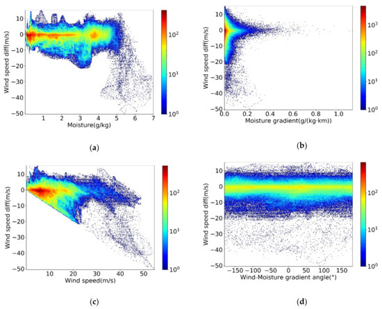
Figure 11.
The wind speed AE as a function of water vapor content (a), water vapor gradient (b), wind speed (c), and wind–moisture gradient angle (d) at 400 hPa.
3.5. Error Comparison by Using Different Types of Water Vapor Data
Though both relative humidity and specific humidity characterize the water vapor, previous analyses are based on specific humidity. The relative humidity is defined as the ratio of water vapor pressure to saturated water vapor pressure, which is also affected by temperature changes. In this session, both water vapor variables are used to calculate the AMVs’ error. Figure 12a,b represent the wind-speed RE at different heights and time intervals tracked using relative humidity and specific humidity, respectively. It is found that the error of using specific humidity is significantly smaller than that of using relative humidity at nearly all heights. In particular, the error of upper and lower layers and the sensitivity of the error to the time resolution are reduced significantly by using specific humidity. This could be attributed to the continuous heat transfer among the upper and lower layers in severe convective areas, resulting in large temperature fluctuations. Therefore, the specific humidity can more accurately describe the water vapor change and movement, comparing with relative humidity, especially under convective areas.
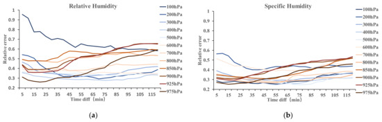
Figure 12.
Wind speed RE at different heights and time intervals by using relative humidity (a) and specific humidity (b) is a figure.
3.6. Error Comparison by Using Water Vapor and Brightness Temperature Data
To confirm that our OF wind-tracking algorithm is suitable for the wind retrieval from MW instruments, we track the simulated MWHS brightness temperature to retrieve winds. We calculate the wind speed RE (Figure 13a), wind speed RMSE (Figure 13b), and the wind direction AE (Figure 13c) of the five layers listed in Table 2. The errors based on BT and water vapor profiles are shown as dash and solid lines, respectively, in Figure 13, with different colors indicating varying vertical heights. The general tendency of two data errors is basically the same. With the time interval flowing, the wind speed RE changes very gently. The wind speed RMSE increases slowly and the wind direction AE decreases slowly over time. The wind speed and wind direction errors from tracking BT and water vapor have the same tendency and distribution with heights. For instance, the largest wind speed error of BT and water vapor all occur at 600 hPa, and the least error is present at 800 hPa. While the OF wind-tracking algorithm can be used for microwave sounding instruments, the wind speed and wind direction errors of using BT are larger than that of using water vapor data. The uncertainty in the height assignment of BT data could be part of error sources. Since BT at 183 GHz is affected by atmospheric variables such as water vapor and temperature profiles, its change with time is a direct reflection of water vapor movement in the atmosphere.
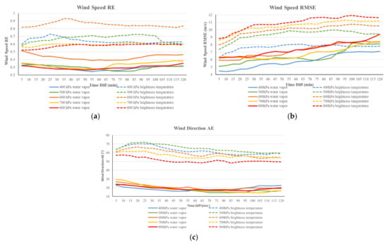
Figure 13.
Wind speed RE (a), wind speed RMSE (b), and wind direction AE (c) at different heights and time intervals by using water vapor and brightness temperature.
In addition, BT simulated by the radiative transfer model also suffers from the systematic errors in atmosphere gaseous absorption, cloud and precipitation scattering, and emission. Brogniez et al. [36] discussed the systematic errors and uncertainties between 183 GHz simulations through radiative transfer model and spaceborne measurements. The channel dependent errors located in the wings of line are nearly 3 K larger than those in the center of the line. Brightness temperatures at the wings of the 183.31 GHz water vapor absorption band are mainly sensitive to the lower tropospheric humidity. Therefore, the systematic errors are larger in the lower troposphere As for the water vapor data simulated by WRF model; we also ignored the turbulence in the microwave instrument FOV. Calbet et al. [37] compared the radiative transfer modeling errors at 183 GHz of the inhomogeneous and uniform FOVs. The results show that the turbulent nature of water vapor is a critical factor in simulations, and the biases are also frequency-dependent. The turbulence in the upper troposphere, storm, or cumulus clouds can cause large water vapor inhomogeneity and result in large errors in the upper atmosphere. The larger inhomogeneity of water vapor retrieved from microwave sounding instruments may be purely a result of the scan-angle dependent FOV. Meanwhile, the different weather conditions from clear to cloud and rain conditions can influence the accuracy of water vapor retrieval, especially in the typhoon area [23]. Since the geostationary microwave observation data are not available yet, we choose to use the simulated BT data and WRF water vapor data for our current experiments.
4. Conclusions
This study explores the potential of the satellite microwave sounding data for tracking the atmospheric winds. The Farenback OF wind-tracking algorithm is developed to obtain an all-sky 3D wind field of Typhoon Lekima and its surrounding areas. The sensitivity of wind-tracking errors is expressed as a function of satellite revisiting time and FOV sizes. The relationships between wind retrieval error and water vapor content, water vapor gradient, wind speed, and wind–moisture gradient angles are analyzed as well. Our conclusions are summarized as follows:
- Specific humidity is suggested to be used as a water vapor tracer to obtain wind field, especially under convective areas. Compared with relative humidity, specific humidity is less affected by temperature changes and more accurately characterizes water vapor changes and movement. Tracking specific humidity features can achieve a more accurate wind field.
- The wind retrieval error decreases as the FOV size decreases, and the error sensitivity to the satellite revisiting time gradually increases. Therefore, if the sensor’s spatial resolution is extremely poor, shortening the revisiting time will not improve the wind field results.
- For fast-evolving weather systems such as typhoons, the Farneback OF wind-tracking algorithm requires a very fine satellite revisiting time. In the central area of the typhoon, due to the fast-moving water vapor field with vertical convergence and divergence, the error is reduced with shorter temporal–spatial resolution.
- For the non-typhoon areas where the water vapor movement is relatively stable, the water vapor field with a time interval of at least 30 min is tracked for conducting a more accurate wind field. The difference between images is too subtle to be identified at a short revisiting time. The algorithm noise will seriously interfere with the signal, which leads to a large proportion of the signal and large retrieval errors.
- The Farneback OF wind-tracking algorithm can realize pixel-wise tracking. It can still obtain an accurate wind field when water vapor content is very low or the wind direction is parallel to the moisture gradient. Compared with the traditional wind-tracking method, our algorithm is more accurate for broader applications.
- The error of tracking simulated BT is larger than that of tracking WRF water vapor fields. Height assignment uncertainty, inclusion of temperature fields, and the systematic errors of BT simulated by radiative transfer model may increase the errors. After the geostationary microwave sounder data are available, the retrievals will consider accuracy, the uncertainty in water valor inhomogeneity, scan angle, and various weather events so that a high quality of water vapor field can be derived for wind tracking.
As Farneback (2003) pointed out, the main disadvantage of the algorithm is its assumption of the slowly changing displacement field, resulting in image discontinuities being smoothed. Thus, a certain error still exists in a relatively flat water vapor area with a short revisiting time. Future work will consider combining some image segmentation methods to amplify the small displacements in these areas to reduce the noise proportion and improve the accuracy. The current microwave measurements mainly rely on polar-orbiting satellites of which the time resolution cannot meet the demand for wind tracking. However, the Farneback OF wind-tracking algorithm in this study is ready for the applications of future geostationary microwave sounders and a constellation of more small satellites cubesats to obtain more accurate atmospheric 3D wind fields.
Author Contributions
Conceptualization, F.W. and H.H.; writing—original draft preparation, Y.Z. All authors have read and agreed to the published version of the manuscript.
Funding
This research was funded by the National Key Research and Development Program of China Development of Meteorological Satellite Remote Sensing Technology and Platform for Global Monitoring, Assessments and Applications under the funding code of 2018YFC1506501.
Conflicts of Interest
The authors declare no conflict of interest.
References
- Van Kuik, G.; Peinke, J.; Nijssen, R.; Lekou, D.; Mann, J.; Sørensen, J.N.; Ferreira, C.; van Wingerden, J.-W.; Schlipf, D.; Gebraad, P. Long-term research challenges in wind energy—A research agenda by the European Academy of Wind Energy. Wind Energy Sci. 2016, 1, 1–39. [Google Scholar] [CrossRef]
- Abrams, D.I. The therapeutic effects of Cannabis and cannabinoids: An update from the National Academies of Sciences, Engineering and Medicine report. Eur. J. Intern. Med. 2018, 49, 7–11. [Google Scholar] [CrossRef]
- Santek, D.; Key, J.; Velden, C.; Bormann, N.; Thépaut, J.-N.; Menzel, W.P. Deriving Winds from Polar Orbiting Satellite Data. In Proceedings of the 6th International Winds Workshop, Madison, WI, USA, 7–10 May 2002; pp. 7–10. [Google Scholar]
- Meissner, T.; Ricciardulli, L.; Manaster, A. Tropical Cyclone Wind Speeds from WindSat, AMSR and SMAP: Algorithm Development and Testing. Remote Sens. 2021, 13, 1641. [Google Scholar] [CrossRef]
- Chronis, T.; Papadopoulos, V.; Nikolopoulos, E. QuickSCAT observations of extreme wind events over the Mediterranean and Black Seas during 2000–2008. Int. J. Climatol. 2011, 31, 2068–2077. [Google Scholar] [CrossRef]
- Gao, Y.; Sun, J.; Zhang, J.; Guan, C. Extreme Wind Speeds Retrieval Using Sentinel-1 IW Mode SAR Data. Remote Sens. 2021, 13, 1867. [Google Scholar] [CrossRef]
- Quartly, G.D.; Chen, G.; Nencioli, F.; Morrow, R.; Picot, N. An Overview of Requirements, Procedures and Current Advances in the Calibration/Validation of Radar Altimeters. Remote Sens. 2021, 13, 125. [Google Scholar] [CrossRef]
- Hautecoeur, O.; Borde, R. Derivation of wind vectors from AVHRR/MetOp at EUMETSAT. J. Atmos. Ocean. Technol. 2017, 34, 1645–1659. [Google Scholar] [CrossRef]
- Santek, D.; Nebuda, S.; Stettner, D. Demonstration and Evaluation of 3D Winds Generated by Tracking Features in Moisture and Ozone Fields Derived from AIRS Sounding Retrievals. Remote Sens. 2019, 11, 2597. [Google Scholar] [CrossRef]
- Ma, Z.; Maddy, E.S.; Zhang, B.; Zhu, T.; Boukabara, S.A. Impact assessment of Himawari-8 AHI data assimilation in NCEP GDAS/GFS with GSI. J. Atmos. Ocean. Technol. 2017, 34, 797–815. [Google Scholar] [CrossRef]
- Velden, C.S.; Olander, T.L.; Wanzong, S. The impact of multispectral GOES-8 wind information on Atlantic tropical cyclone track forecasts in 1995. Part I: Dataset methodology, description, and case analysis. Mon. Weather Rev. 1998, 126, 1202–1218. [Google Scholar] [CrossRef]
- Wang, Y.; He, J.; Chen, Y.; Min, J. The Potential Impact of Assimilating Synthetic Microwave Radiances Onboard a Future Geostationary Satellite on the Prediction of Typhoon Lekima Using the WRF Model. Remote Sens. 2021, 13, 886. [Google Scholar] [CrossRef]
- Fujita, T.T.; Watanabe, K.; Izawa, T. Formation and structure of equatorial anticyclones caused by large-scale cross-equatorial flows determined by ATS-I photographs. J. Appl. Meteorol. Climatol. 1969, 8, 649–667. [Google Scholar] [CrossRef][Green Version]
- Endlich, R.; Wolf, D.; Hall, D.; Brain, A. Use of a pattern recognition technique for determining cloud motions from sequences of satellite photographs. J. Appl. Meteorol. Climatol. 1971, 10, 105–117. [Google Scholar] [CrossRef][Green Version]
- Leese, J.A.; Novak, C.S.; Clark, B.B. An automated technique for obtaining cloud motion from geosynchronous satellite data using cross correlation. J. Appl. Meteorol. Climatol. 1971, 10, 118–132. [Google Scholar] [CrossRef]
- Menzel, W.P.; Merrill, R.T. The NESDIS/CIMSS wind algorithm: Current status and future improvements. In Proceedings of the Workshop on Wind Extraction from Operational Meteorological Satellite Data, Madison, WI, USA, 17–19 September 1991; pp. 10–77. [Google Scholar]
- Mueller, K.; Moroney, C.; Jovanovic, V.; Garay, M.; Muller, J.; Di Girolamo, L.; Davies, R. MISR Level 2 Cloud Product Algorithm Theoretical Basis; JPL Tech. Doc. JPL D-73327; Jet Propulsion Laboratory: La Cañada Flintridge, CA, USA, 2013.
- Xu, J.; Holmlund, K.; Zhang, Q.; Schmetz, J. Comparison of two schemes for derivation of atmospheric motion vectors. J. Geophys. Res. Atmos. 2002, 107, ACL 4-1–ACL 4-15. [Google Scholar] [CrossRef]
- Mueller, K.J.; Wu, D.L.; Horváth, Á.; Jovanovic, V.M.; Muller, J.-P.; Di Girolamo, L.; Garay, M.J.; Diner, D.J.; Moroney, C.M.; Wanzong, S. Assessment of MISR cloud motion vectors (CMVs) relative to GOES and MODIS atmospheric motion vectors (AMVs). J. Appl. Meteorol. Climatol. 2017, 56, 555–572. [Google Scholar] [CrossRef]
- Salonen, K.; Cotton, J.; Bormann, N.; Forsythe, M. Characterising AMV height assignment error by comparing best-fit pressure statistics from the Met Office and ECMWF system. In Proceedings of the 11th International Wind Workshop, Auckland, New Zealand, 20–24 February 2012. [Google Scholar]
- Santek, D.; Nebuda, S.; Stettner, D. Feature-tracked winds from moisture fields derived from AIRS sounding retrievals. In Proceedings of the 12th International Winds Workshop, Copenhagen, Denmark, 15–20 June 2014. [Google Scholar]
- Hu, H.; Weng, F.; Han, Y.; Duan, Y. Remote sensing of tropical cyclone thermal structure from satellite microwave sounding instruments: Impacts of background profiles on retrievals. J. Meteorol. Res. 2019, 33, 89–103. [Google Scholar] [CrossRef]
- Hu, H.; Han, Y. Comparing the Thermal Structures of Tropical Cyclones Derived from Suomi NPP ATMS and FY-3D Microwave Sounders. IEEE Trans. Geosci. Remote Sens. 2020. [Google Scholar] [CrossRef]
- Lin, L.; Weng, F. Estimation of hurricane maximum wind speed using temperature anomaly derived from Advanced Technology Microwave Sounder. IEEE Geosci. Remote Sens. Lett. 2018, 15, 639–643. [Google Scholar] [CrossRef]
- Ma, Y.; Zou, X.; Weng, F. Potential applications of small satellite microwave observations for monitoring and predicting global fast-evolving weathers. IEEE J. Sel. Top. Appl. Earth Obs. Remote Sens. 2017, 10, 2441–2451. [Google Scholar] [CrossRef]
- Wang, S.; Shi, S.; Ni, B. Joint Use of Spaceborne Microwave Sensor Data and CYGNSS Data to Observe Tropical Cyclones. Remote Sens. 2020, 12, 3124. [Google Scholar] [CrossRef]
- Lambrigtsen, B.; Van Dang, H.; Turk, F.J.; Hristova-Veleva, S.M.; Su, H.; Wen, Y. All-weather tropospheric 3-D wind from microwave sounders. IEEE J. Sel. Top. Appl. Earth Obs. Remote Sens. 2018, 11, 1949–1956. [Google Scholar] [CrossRef]
- Posselt, D.J.; Wu, L.; Mueller, K.; Huang, L.; Irion, F.W.; Brown, S.; Su, H.; Santek, D.; Velden, C.S. Quantitative Assessment of State-Dependent Atmospheric Motion Vector Uncertainties. J. Appl. Meteorol. Climatol. 2019, 58, 2479–2495. [Google Scholar] [CrossRef]
- Sun, F.; Min, M.; Qin, D.; Wang, F.; Hu, J. Refined typhoon geometric center derived from a high spatiotemporal resolution geostationary satellite imaging system. IEEE Geosci. Remote Sens. Lett. 2018, 16, 499–503. [Google Scholar] [CrossRef]
- Farnebäck, G. Two-frame motion estimation based on polynomial expansion. In Proceedings of the Scandinavian Conference on Image Analysis, Halmstad, Sweden, 29 June–2 July 2003; pp. 363–370. [Google Scholar]
- Farnebäck, G. Polynomial Expansion for Orientation and Motion Estimation; Linköping University Electronic Press: Linköping, Sweden, 2002. [Google Scholar]
- Brox, T.; Bruhn, A.; Papenberg, N.; Weickert, J. High accuracy optical flow estimation based on a theory for warping. In Proceedings of the European Conference on Computer Vision, Prague, Czech Republic, 11–14 May 2004; pp. 25–36. [Google Scholar]
- Burt, P.J.; Adelson, E.H. The Laplacian pyramid as a compact image code. In Readings in Computer Vision; Elsevier: Amsterdam, The Netherlands, 1987; pp. 671–679. [Google Scholar]
- Baker, N.L. Quality control for the navy operational atmospheric database. Weather Forecast. 1992, 7, 250–261. [Google Scholar] [CrossRef]
- Saucier, W.J. Principles of Meteorological Analysis; University of Chicago Press: Chicago, IL, USA, 1955. [Google Scholar]
- Brogniez, H.; English, S.; Mahfouf, J.-F.; Behrendt, A.; Berg, W.; Boukabara, S.; Buehler, S.A.; Chambon, P.; Gambacorta, A.; Geer, A. A review of sources of systematic errors and uncertainties in observations and simulations at 183 GHz. Atmos. Meas. Tech. 2016, 9, 2207–2221. [Google Scholar] [CrossRef]
- Calbet, X.; Peinado-Galan, N.; DeSouza-Machado, S.; Kursinski, E.R.; Oria, P.; Ward, D.; Otarola, A.; Rípodas, P.; Kivi, R. Can turbulence within the field of view cause significant biases in radiative transfer modeling at the 183 GHz band? Atmos. Meas. Tech. 2018, 11, 6409–6417. [Google Scholar] [CrossRef]


Publisher’s Note: MDPI stays neutral with regard to jurisdictional claims in published maps and institutional affiliations. |
© 2021 by the authors. Licensee MDPI, Basel, Switzerland. This article is an open access article distributed under the terms and conditions of the Creative Commons Attribution (CC BY) license (https://creativecommons.org/licenses/by/4.0/).