Abstract
Detection of aircrafts in satellite images is a challenging problem when the background is strongly reflective clouds with varying transparency. We develop a fast and effective detection algorithm that can find almost all aircrafts above and between clouds in Sentinel-2 multispectral images. It exploits the time delay of a few seconds between the recorded multispectral images such that a moving aircraft is observed at different positions due to parallax effects. The aircraft speed, heading and altitude are also calculated accurately. Analysing images over the English Channel during fall 2020, we obtain a detection accuracy of 80%, where the most of the remaining were covered by clouds. We also analyse images in the 1.38 μm water absorption band, where only 61% of the aircrafts are detected.
Keywords:
remote sensing; Sentinel-2; multispectral imaging; aircrafts; velocities; clouds; parallax; planebow 1. Introduction
Surveillance for air space situational awareness is essential for monitoring and controlling air traffic and its climate impact. Dark aircrafts are non-cooperative vessels with non-functioning transponder systems, such as the automatic dependent surveillance broadcast (ADS-B) [1] or similar devices. Their transmission may have temporal gaps or be jammed, spoofed, sometimes experience erroneous returns, or simply be turned off deliberately or by accident. Furthermore, ADS-B is mostly land-based and satellite coverage at open sea and at high latitudes is sparse, which means that other surveillance systems such as satellite systems are required. Numerous satellites in low-Earth orbits provide Earth observation images with good resolution, such as the Sentinels [2]. Most are in polar orbits, where the swaths from different satellite orbits overlap at higher latitudes, and the resulting frequent transits over the polar regions make these satellites particularly useful for Arctic surveillance. Aircrafts and ships cannot hide from satellites unless they are stealth in radio and multispectral spectral bands.
The literature on aircraft detection in satellite images concentrates on aircrafts on the ground in airports, where elaborate detection algorithms have been developed (see, e.g., [3,4] and refs. herein). Detection of flying aircrafts from satellites has only been studied for Landsat data in the 1.38 μm band [5] and for Sentinel-2 (S2) mostly cloud-free images [3,6,7].
Cloud cover inhibits optical detection from satellites and, therefore, cloud-penetrating synthetic aperture radars (SAR) are most commonly used for ship detection, although their resolution generally is worse than optical sensors and the number of bands is fewer. However, the SAR recording technique displaces sailing ships proportionally to their speed by hundreds of meters [8] and this would make the detection of fast-flying aircrafts even more difficult.
Since aircrafts fly above clouds most of the time, they can be detected by optical sensors. However, the underlying cloud background can be highly reflective with spatially varying albedo, which makes detection a challenging problem. The purpose of this work is to find robust, effective, and optimal methods for detecting and classifying aircrafts in S2 images with clouds, and to determine their velocities and altitudes.
2. Satellite Images and Method of Analysis
To demonstrate our flying aircraft detection method, we shall use data from the Sentinel-2 (S2) satellites under the Copernicus program [2] as Figure 1. They provide excellent and freely available imagery with pixel resolutions down to 10 m in 13 multispectral bands. The orbital periods are 5 days between the S2 satellites A + B, but revisit up to daily in polar regions due to overlapping swaths.
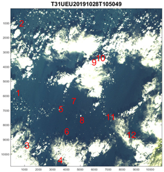
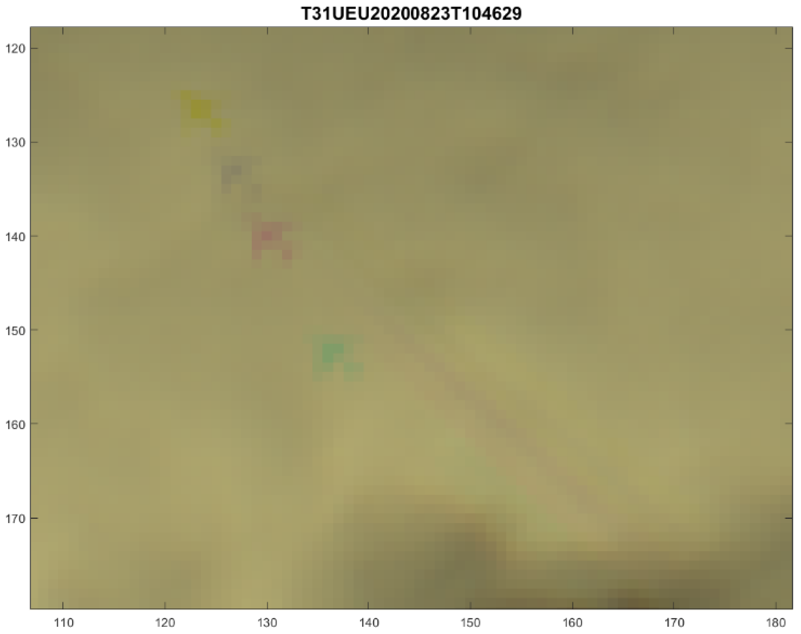
Figure 1.
RGB image of the S2 tile T31UEU over the English Channel, 28 October 2019, 10:56:30 UTC. Red numbers indicate the positions of the 12 detected aircraft. Axes are pixel numbers.
2.1. Sentinel-2 Multispectral Images
We analyse S2 Level-1C top-of-atmosphere images, which are not corrected for aerosol reflections, atmospheric moisture absorption, or clouds, and contain the water absorption band around 1.38 μm. We choose scenes over the English Channel (see Figure 1), where the air traffic is dense and cloud cover frequent. All scenes covering this tile are analysed over a period between 16 August and 20 October in 2020 as well as the scene of Figure 1 from before the COVID-19 pandemic, when the air traffic was more than double. The recording time of the image is 15 s and we match with ADS-B in this time interval so that the positions match for the fast-flying aircrafts. The time T105049 in the Sentinel filenaming convention shown above Figure 1 is the data’s start sensing time. The actual tile image scene is recorded almost six minutes later at 10:56:30 UTC. Because the aircrafts fly so fast, we can determine this time by comparing to ADS-B, with accuracy down to a few seconds. We can even observe the 15 s recording time difference from top to bottom. The correct timing is done once and for all for Sentinel 2A and 2B separately as they differ.
The S2 Multispectral Sensor Imager (MSI) [2] records images in 13 multispectral bands (see Table 1) with different resolutions and time delays due to their push-broom recording technique. There are 4 bands with 10 m, 6 bands with 20 m, and 3 bands with 60 m pixel resolution. These are giga-pixel scenes with 12-bit grey levels. The spatial coordinates are the pixel coordinates (i, j) multiplied by the pixel resolution l = 10 m, 20 m, or 60 m for the S2 multispectral images , in the 13 bands. The bands are time-ordered according to temporal offset , m = 1,…, 13, with respect to the blue band, as shown in Table 1.

Table 1.
The 13 spectral bands for S2-B MSI ordered according to wavelength and temporal delay tm, m = 1,…, 13.
2.2. Background Subtraction
Aircraft detection was analysed in [6] over sea for clear sky. The dark sea background made it easy to detect aircrafts (and ships) and accurately determine their velocities and altitudes. In a highly reflective cloud background with varying albedo, the simple threshold detection method of [6] fails because the clouds’ reflection exceeds the threshold.
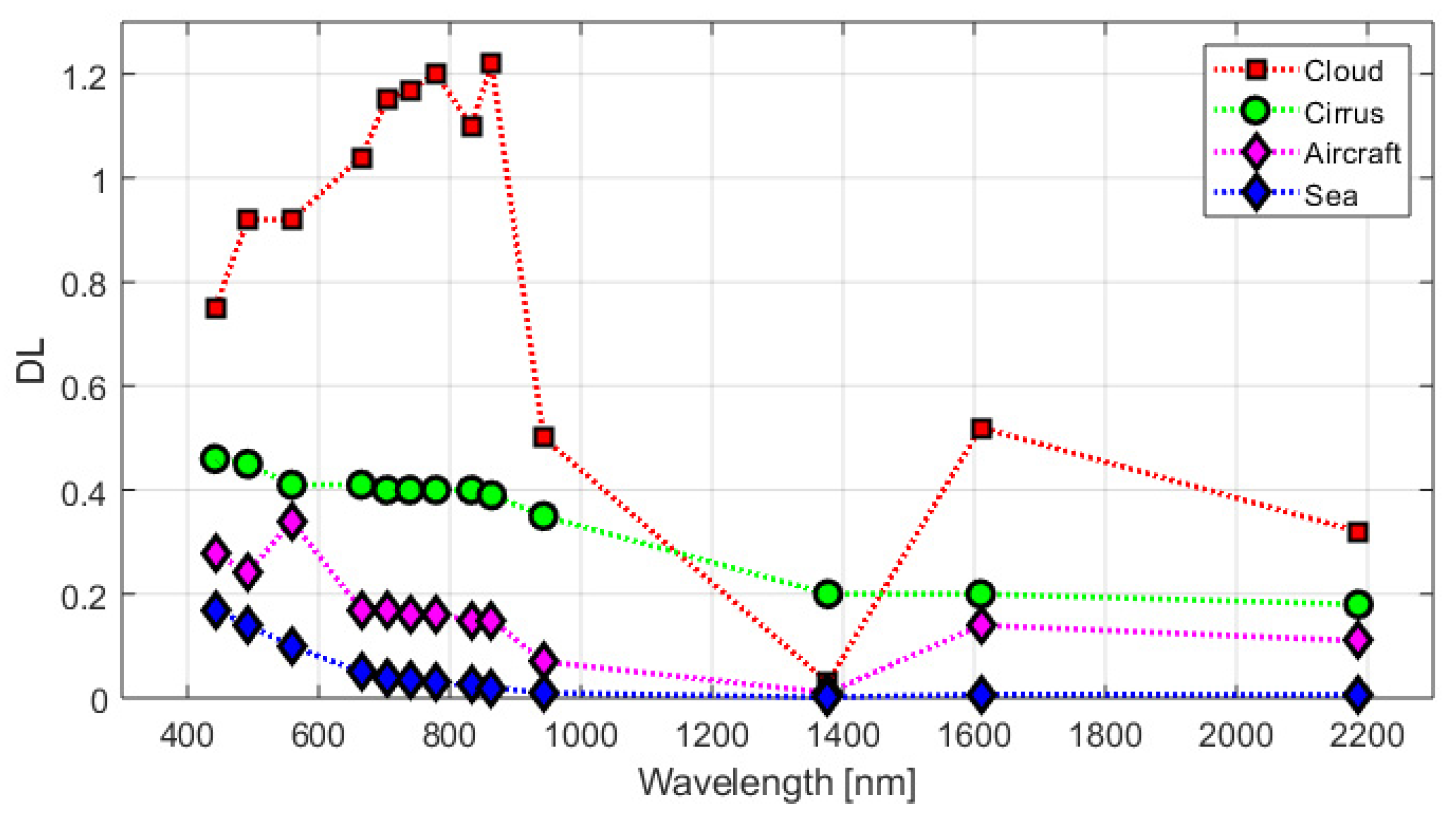
In order to construct an effective aircraft detection algorithm, one must first understand the reflection spectra for the backgrounds. As shown in Figure 2, the sea reflection decreases with wavelength, whereas the reflection from clouds is stronger at larger wavelengths. As the cloud altitudes and thicknesses vary, we observe mixed spectra from low to high reflective and cirrus clouds.
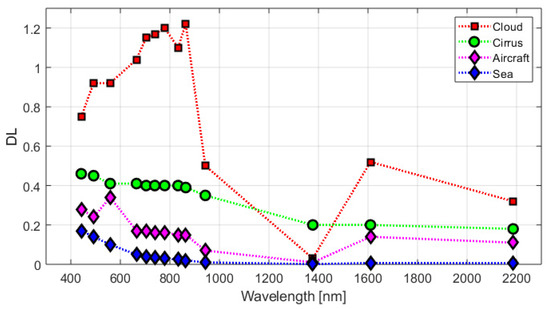
To determine how the aircrafts change the spectrum relative to a background, we define the background spectrum vectors , where the index i = 1,…, N, refers to sea, various types of clouds, snow, or land. Examples are shown in Figure 2. As the background can be a mixture of these spectra, we multiply them by weights , i = 1,…, N, and subtract
The weights are determined for each pixel by minimising the mean square of Equation (1), which corresponds to an N-parameter linear regression fit or a spectral mixture analysis. The resulting weights are: , where is the inverse of the N × N matrix with elements , where the i = 1,…, N and j = 1,…, N indices both refer to sea, clouds, or other background spectra, and the dot is a vector product of up to M = 13 multispectral band vectors. The background-subtracted spectrum displays the change due to the aircraft, as shown in Figure 3 and Figure 4.

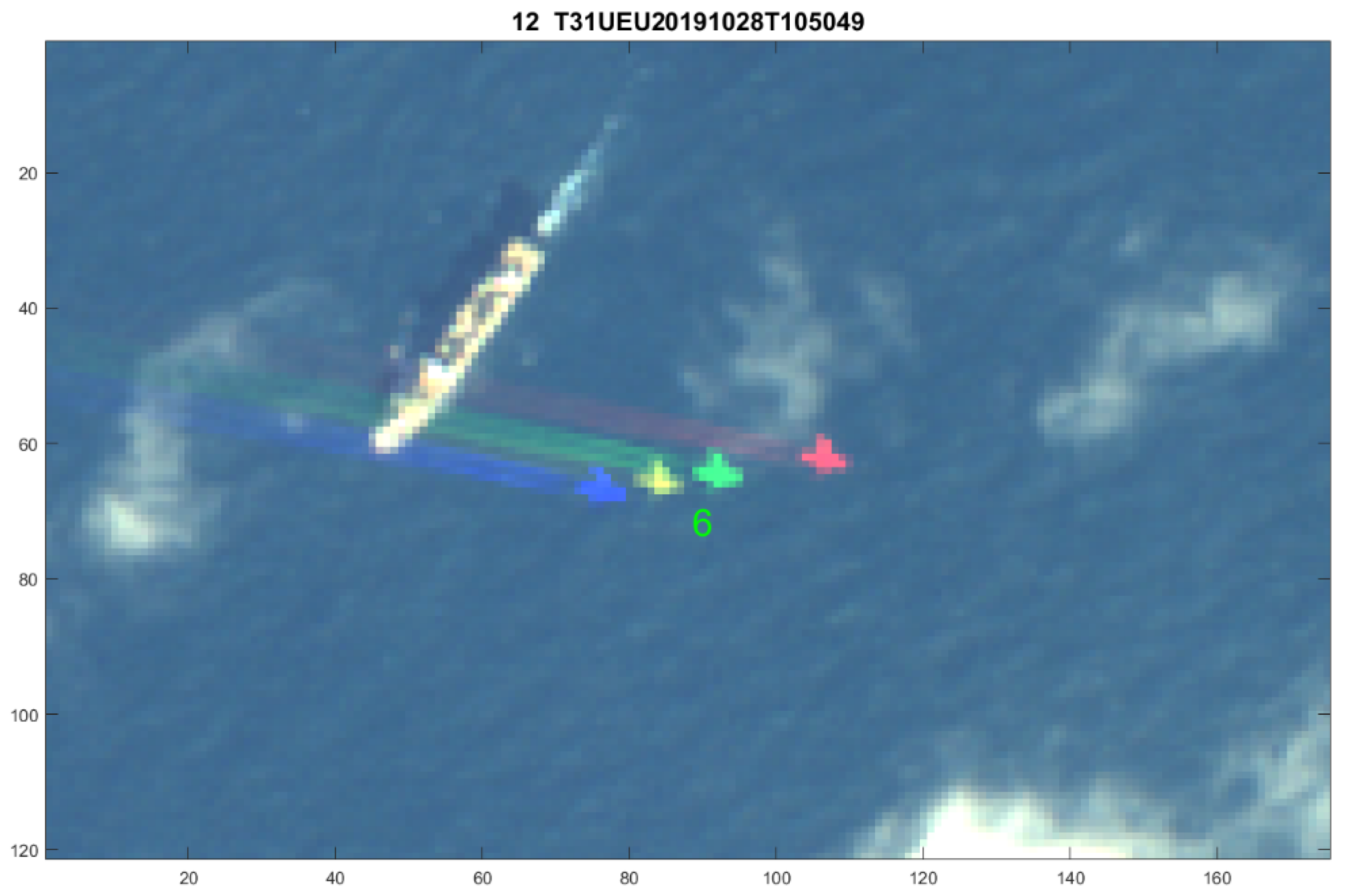
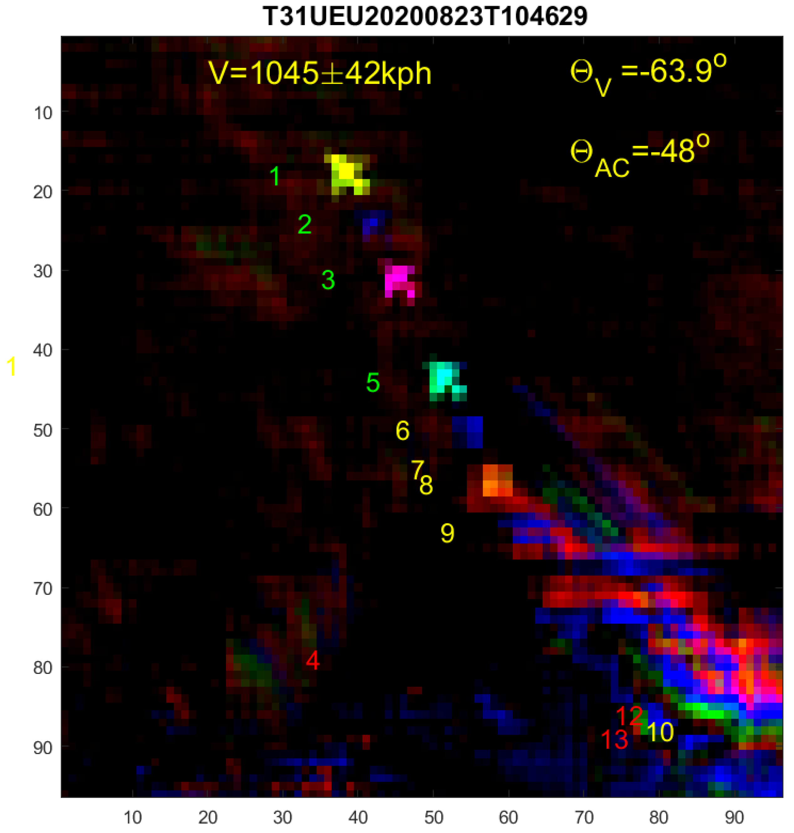
Figure 3.
Closer look at aircraft #5 of Figure 1 with a background of sea, clouds, and a ship. The m = 2 band is stacked by yellow. Contrails form a rainbow due to the satellite parallax effect, and the aircraft moves forward due to time delays.

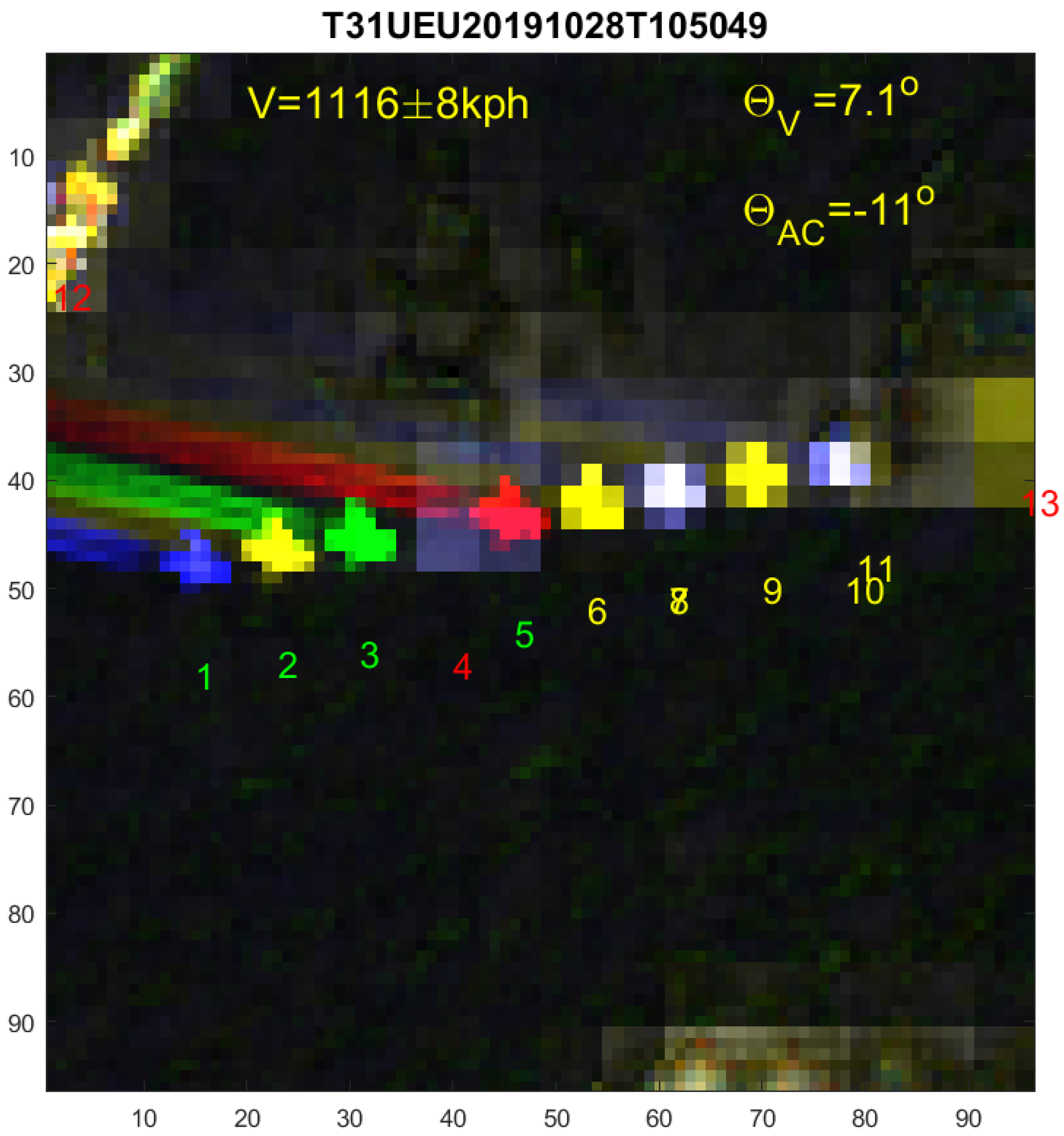
Figure 4.
Background-subtracted image of Figure 3, where the sea and clouds are effectively removed. Red, green, and blue are true colours whereas the 10 remaining are stacked as false colours (alternating yellow and white). Due to parallax effects, the aircraft shows up 13 times on a line. Contrails from each wing motor form a planebow and clearly indicate the angle for the aircraft velocity VAC direction. Numbers m = 1,…, 13 indicate central aircraft position in each time ordered band (but moved 10 pixels down). Green, yellow, and red numbers refer to high-, medium-, and low-resolution bands, respectively. Note that 12 is misplaced to the ship, and 7 and 8 are almost on top because they are recorded almost simultaneously.
2.3. Multispectral Temporal Offsets, Positions, and Velocities
From the background-subtracted spectra, the positions in each band m = 1,…, 13, are determined as the central object coordinate and we also determine its orientation angles .
An object moving with apparent velocity will ideally be recorded at position
Here, is the vessel position at zero temporal offset—ideally, the blue band for which (see Table 1). The object positions that are calculated for each multispectral image will generally scatter around the linear prediction of Equation (2). We define the variance as the mean square average of the deviations
Ideally, M = 13, when all bands are included, but in cloudy backgrounds, the low-resolution bands often fail, and we therefore sum the four high-resolution bands only as they are more precise. By minimising this variance, which is equivalent to a two-parameter linear regression, we obtain the best fit values for aircraft position and apparent velocity vector .
The apparent velocity vector is , and contains two parallax effects due to the aircraft and satellite motion, as described in [6]. The S2 satellites fly in a sun-synchronous orbit at mean altitude of HS2 = 786 km with speed VS2 = 7.44 km/s, descending with inclination angle = −104° at the latitude of the English Channel [6]. During the multispectral delay, the aircraft and its contrails are moved with respect to the ground by the parallaxes depending on the aircraft velocity , and altitude HAC. The aircraft and its condensation stripes are separated for each multispectral band and appear as a “planebow”, when all bands are stacked in a false colour image, as shown in Figure 4, and the aircraft shows up as 13 pearls on a string along .
As result, we find the aircraft velocity [6]
and altitude
The aircraft heading angle may be determined from the aircraft orientation angles discussed above, and/or by the condensation trails, which are visible at altitudes 7.5–11 km (see Figure 3). See [6] for the more complicated case including jet streams.
Flying aircrafts are special because of the temporal delay between recordings. For example, a pixel covering the aircraft when the green band is recorded will have a peak at the green wavelength but be lower in all other bands (see Figure 2), and likewise for the other bands. The difference between bands in pixel reflection is therefore a good measure of the change due to parallax effects and can be exploited for aircraft detection. However, numerous false alarms occur from clouds with relatively sharp boundaries due to the satellite parallax. We find that these false alarms are minimal for the difference between the green and blue bands as they are recorded with a 0.527 s time difference only so that the cloud parallax change is smallest. As seen in Figure 2, the aircraft increases its DL by ca. 20% in the green band, and we find an optimal threshold of T = 0.05 DL in order to detect most aircraft without too many false alarms (see Figure 1).
Adjacent detected pixels are connected to objects. For each object, a small 96 × 96 pixel clip is selected around the central object coordinate, which covers the aircraft extent, including movement and part of its condensation trail (see [6] for details). The same 960 × 960 m region is now extracted for all 13 bands, and we construct the spectral reflection vector for each pixel; see Figure 4.
2.4. The Parallax Method
For optimising the aircraft detection and classification in S2 images, we employ the following parallax method or algorithm:
- For a given scene, the multispectral S2 images are collected from [2].
- Change detection of objects by the green–blue difference above threshold .
- For each object, a clip is extracted in the four high-resolution bands with background subtraction; see Equation (1).
- For each clip, V, , , , and are calculated from Equations (2)–(5).
- False alarms are removed by requiring high velocity V > 100 m/s and low scatter σ < V/5.
- Positions , , and are compared to ADS-B numbers for aircrafts at the same place and time.
To speed up the algorithm, only two images are used in step 2, and only the clips for the four high-resolution images (M = 4) are analysed in steps 3 and 4. Over sea, we only subtract sea and the dominant cloud background in the clip, i.e., N = 2. For better but slower analysis in a less cloudy background, the algorithm can run with more multispectra (M) and background subtractions (N) up to 13.
Step 5 is essential because step 2 results in a large number of false alarms, especially in images with cauliflower clouds as their edges are prone to the parallax effect. However, their positions are much more irregular, whereas aircrafts appear as pearls on a string. This is exploited by the high velocity and low scatter conditions, which effectively removes most false alarms. The false alarm threshold σ < V/5 is chosen by experience in order to reduce false alarms maximally while retaining most aircrafts. This results in high recall values.
2.5. The Water Absorption Band at 1.38 μm
As described in [5], the 1.38 μm band is also useful for detecting high-altitude aircrafts. Water in the atmosphere absorbs strongly at this wavelength and suppresses the background from the surface of the Earth as well as low-lying clouds, whereas high-altitude aircrafts are unaffected and thus contrast enhanced. The aircraft spectrum in Figure 2 is for a pixel at the green aircraft position of Figure 3 and Figure 4 and therefore the spectrum has enhanced for band 3. For a pixel at the aircraft position in the 1.38 μm band, the spectrum would not be zero for band 10 (m = 4) as it would be for all low-altitude objects due to water absorption.
However, whereas the Landsat data in [5] have 30 m pixel resolution, the S2 data have only 60 m resolution in the 1.38 μm band , and aircrafts are therefore detected in very few pixels. When high-altitude clouds are present, they lead to numerous false alarms. We find that subtracting a background smeared over a few pixels suppresses clouds and reduces the number of false alarms considerably.
3. Results
The resulting aircraft detections from manual inspection in the four high-resolution bands, the 1.38 μm band, and the parallax algorithm are now compared to ground truth values from ADS-B.
3.1. Detections and False Alarms
We analysed 27 scenes of the English Channel over a continuous period of two months with varying cloud cover. According to ADS-B, there were 112 aircrafts present in total. We only found one aircraft without an ADS-B signal. The number of detected aircrafts is given in Table 2 vs. cloud cover in five bins. Almost all were found by manual inspection when the cloud cover was low, whereas around half were invisible for strong cloud cover. On average, 80% were observed by manual inspection in the four high-resolution bands. An estimated 10% could not be detected visually as they flew below or in clouds. The remaining 10% of undetected aircrafts may have been covered by high-altitude cirrus clouds or had reflections too close to background clouds. Only one (dark) aircraft without an ADS-B signal was found in all.
Table 2.
The number of detected aircrafts vs. cloud cover by ADS-B, manual inspection, the parallax method, and by manual inspection in the 1.38 μm band.
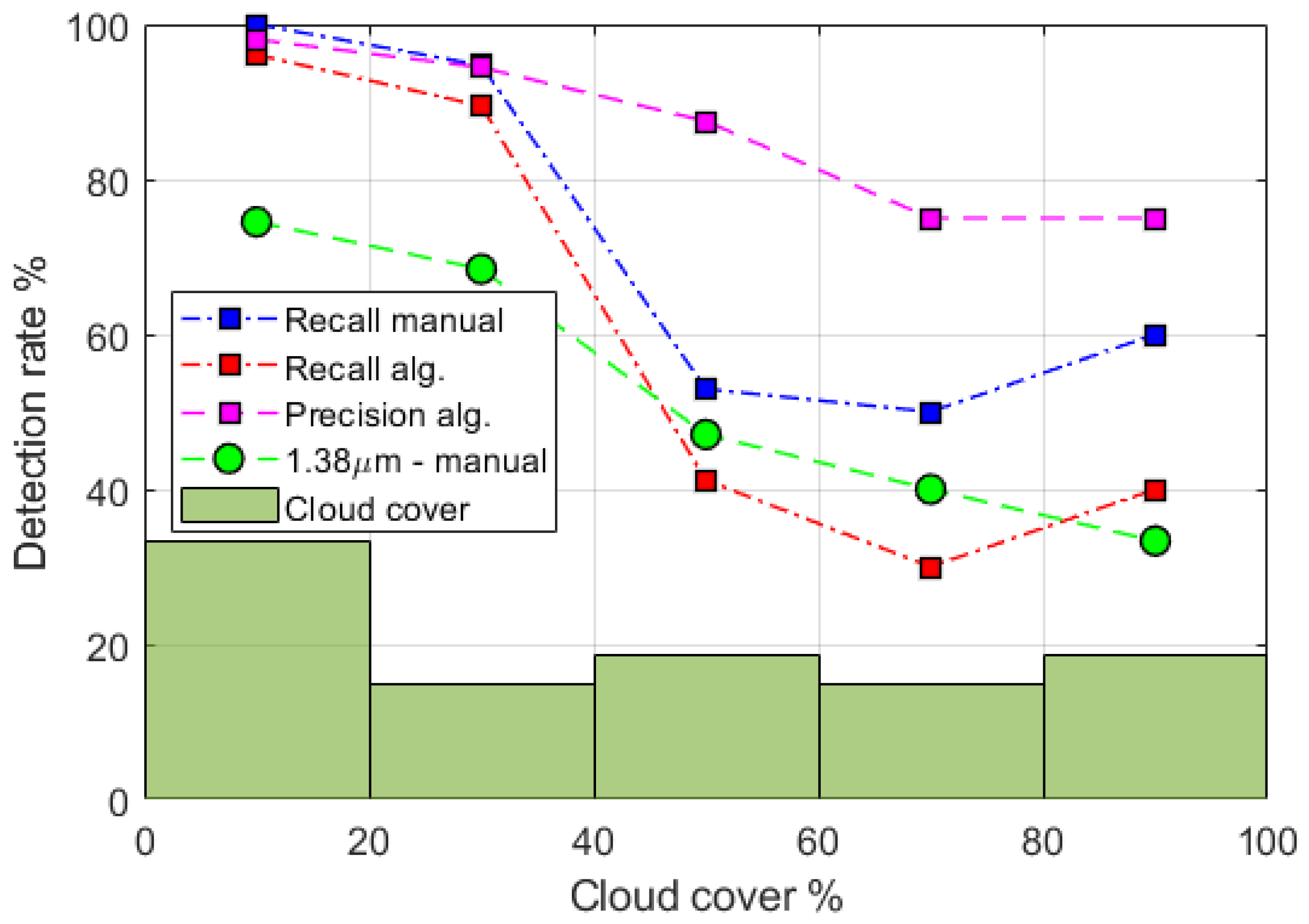
The green–blue parallax algorithm was able to detect most of the aircrafts found by manual inspection, as shown in Figure 5 by the recall, which is the number of detected aircrafts relative to ADS-B for a given cloud cover. The average recall is 73%. There were only seven false alarms by the parallax method, which gives an average precision of 92%. Two aircrafts were less reflective than the cloud background as in Figure 6, requiring inverted detection. Three aircrafts (not included) were only visible by their contrails.
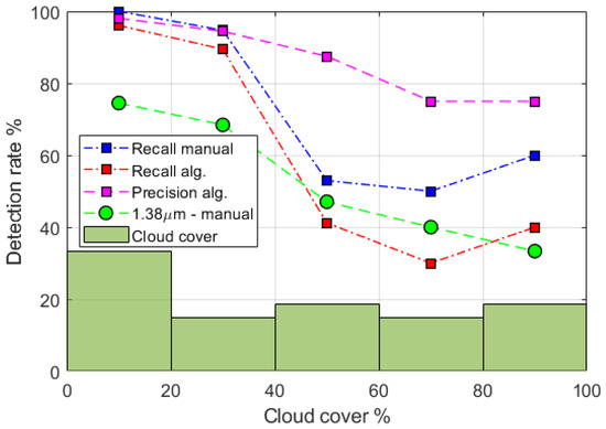
Figure 5.
The detection rates generally decrease with increasing cloud cover. The curves display detection by manual inspection, the parallax method (precision and recall), and manual inspection in the 1.38 μm band. The green bars show the percentage of scenes in the period vs. cloud cover bins.

Figure 6.
As in Figure 3 but for an aircraft above a stronger reflecting cloud such that its colours are inverted.
The number of false alarms from cloud edges was low, except for dense cloud cover. The precision curve in Figure 5 is the detected aircrafts relative to the total number of detections including false alarms. Lowering the threshold T and relaxing the velocity and scatter conditions led to numerous false alarms and lower precision but the recall did not improve by much.
In the 1.38 μm band, only 61% of the aircrafts could be found by manual inspection due to the lower resolution and the fact that some of the low-flying aircrafts became undetectable due to water absorption in the atmosphere even with clear sky. Only two aircrafts seen in the 1.38 μm band were not detected by the parallax method.
3.2. Aircraft Velocity and Altitude
The aircraft velocity and altitude are calculated from Equations (3) and (4). Typically, the aircraft position is determined within a pixel in each multispectral image. The two-dimensional linear regression fit of vs. tm therefore has a standard deviation less than σ ~ 10 m over the temporal delay interval of 2.586 s, which results in an uncertainty for the apparent velocity of ~4 m/s. This is relatively accurate when compared to typical aircraft velocities of 100–300 m/s.
In Figure 3 and Figure 4, the aircraft engines under each wing create two long condensation trails for each band, which determine the aircraft heading angle = −11°, whereas the apparent angle is = 7.1°. It moves a distance of ~80 pixels or 800 m in the time interval of 2.586 s, and thus flies with an apparent speed of V = 310 m/s = 1116 kph with uncertainty σ 8 kph. From Equations (4) and (5), we find the aircraft speed kph and altitude km, in good agreement with ADS-B.
In Figure 6 and Figure 7, an aircraft is detected by the algorithm, but as it is reflecting less than the underlying cloud, its colours are inverted, which we take into account. The scatter σ generally increases in a background of dense clouds, especially for the bands with poor resolution.
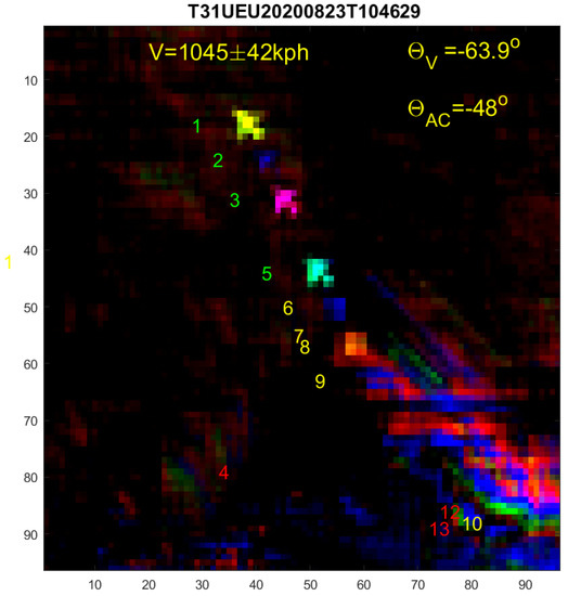
Figure 7.
Background-subtracted Figure 6.
4. Discussion
A direct comparison to the results of [5,7] is difficult because the regions and periods differ, and detection rates depend strongly on the selected scenes and their cloud cover. For example, excluding the last week of October, with dense cloud cover, in our analysis leads to an increase of 10% in the detection rates. As we have included all S2 images in a given tile and two-month period, our results can be used as benchmark in the future.
Aircraft detection was performed for the Landsat 8 OLI 1.38 μm band in [5]. Its 30 m pixel resolution is better than S2, which was exploited in a detailed spatial discrimination algorithm that could detect most large aircrafts above 5 km altitude. Of 566 aircrafts present according to ADS-B, detection rates varied between continents due to varying cloud cover and atmospheric moisture. The worst case was China, where 8% of the aircrafts were not detected manually and 68% were missed by the algorithm. Restricted to the same altitudes and large aircrafts, we missed, on average, 29% by manual inspection in the 1.38 μm band. The larger miss rate reflects the lower resolution.
Liu et al. [7] detected 3724 aircrafts in S2 MSI images from the reflectance differences between the red, green, and blue bands. According to ADS-B [1], there were 5820 aircrafts present, i.e., 40% were not detected. These were mainly smaller and slower aircrafts flying at low altitudes, where cloud cover could explain 72% of the failed detections. For comparison, our method missed 29%, of which all were in a dense background of clouds. The low miss rate is partly due to the inversion method for strong cloud reflection backgrounds. Restricting to cloud-free images, we missed no aircrafts [6]. In the presence of clouds, the method is limited to aircrafts above clouds and with reflections differing from clouds more than the threshold, which cannot be set too low due to false alarms from, e.g., cloud edges.
Note that the aircraft altitudes were not calculated in [7] and their aircraft velocities deviated substantially from those reported by ADS-B especially at high altitudes. This indicates that the satellite parallax effect was omitted. We find good agreement for both altitudes, direction, and velocities, when both the aircraft and satellite parallaxes are included.
5. Summary and Outlook
We designed a parallax method that analyses multispectral images for detecting aircrafts above clouds. It utilises the time delays in multispectral S2 satellite images and is better than detections in the 1.38 μm band. Both methods are fast, robust, and with high detection and low false alarm rates, except for high-altitude clouds. Analysing 27 scenes over the English Channel for a two-month period with 112 aircrafts and comparing to ADS-B, we find 80% by manual inspection and 73% by the parallax method on average. Even contrails and aircrafts above highly reflective clouds could be detected by an inversion method. Aircraft velocity, heading, and altitude were also calculated accurately. In comparison, the 1.38 μm band detected only 61% due to clouds, water absorption in the atmosphere, and lower resolution.
The parallax algorithm can produce a database of aircraft images wherefrom directions, velocities, and altitudes are calculated. These can then be complemented by corresponding ADS-B numbers and form an annotated database for training neural networks. Such more advanced algorithms may further improve the relatively simple spectral change detection yet effective parallax method developed here. Based on this work, we expect that deep learning can improve aircraft detection rates up to or above the manual inspection rates, and may even exceed 90% on average, when aircrafts flying in or below clouds are excluded. This will be investigated in future work.
Author Contributions
Methodology and writing, H.H.; software and formal analysis, P.H. Both authors have read and agreed to the published version of the manuscript.
Funding
This work was in part supported by the Danish Defence and Joint Arctic Command.
Data Availability Statement
From the ESA Copernicus Program [2].
Conflicts of Interest
The authors declare no conflict of interest.
References
- ADS-B: Live Flight Tracker. Available online: https://planefinder.net/ (accessed on 1 July 2021).
- ESA Copernicus Program, Sentinel Scientific Data Hub. Available online: https://schihub.copernicus.eu (accessed on 1 July 2021).
- Skakun, S.; Vermote, E.; Roger, J.-C.; Justice, C. Multispectral Misregistration of Sentinel-2A Images: Analysis and Implications for Potential Applications. IEEE Geosci. Remote Sens. Lett. 2017, 14, 2408–2412. [Google Scholar] [CrossRef] [PubMed]
- Shi, F.; Qiu, F.; Li, X.; Tang, Y.; Zhong, R.; Yang, C. A Method to Detect and Track Moving Airplanes from a Satellite Video. Remote Sens. 2020, 12, 2390. [Google Scholar] [CrossRef]
- Zha, F.; Xia, L.; Kylling, A.; Li, R.Q.; Shang, X.; Xu, M. Detection of flying aircraft from Landsat 8 OLI data. J. Photogramm. Remote Sens. 2018, 141, 176–184. [Google Scholar] [CrossRef]
- Heiselberg, H. Aircraft and Ship Velocity Determination in Sentinel-2 Multispectral Images. Sensors 2019, 19, 2873. [Google Scholar] [CrossRef] [PubMed] [Green Version]
- Liu, Y.; Xu, B.; Zhi, W.; Hu, C.; Dong, Y.; Jin, S.; Lu, Y.; Chen, T.; Xu, W.; Liu, Y.; et al. Space eye on flying aircraft: From Sentinel-2 MSI parallax to hybrid computing. Remote Sens. Environ. 2020, 246, 111867. [Google Scholar] [CrossRef]
- Ouchi, K. On Multilook Images of Moving Targets by Synthetic Aperture Radars. IEEE Trans. Antennas Propag. 1985, 33, 823–827. [Google Scholar] [CrossRef]

Publisher’s Note: MDPI stays neutral with regard to jurisdictional claims in published maps and institutional affiliations. |
© 2021 by the authors. Licensee MDPI, Basel, Switzerland. This article is an open access article distributed under the terms and conditions of the Creative Commons Attribution (CC BY) license (https://creativecommons.org/licenses/by/4.0/).