
Progress in Grassland Cover Conservation in Southern European Mountains by 2020: A Transboundary Assessment in the Iberian Peninsula with Satellite Observations (2002–2019)

 , ,
, ,  ,
,  ,
,  and
and
Abstract
:1. Introduction
- (1)
- What is the progress made in grassland cover conservation by 2020 according to the extent and net shift observed between 2002 and 2019?
- (2)
- To what extent do protected and unprotected land governance regimes differ in grassland cover conservation?
- (3)
- What is the accuracy level of MCE approaches in mountain grasslands? What is the relationship between class-allocation uncertainty and classification accuracy?
2. Materials and Methods
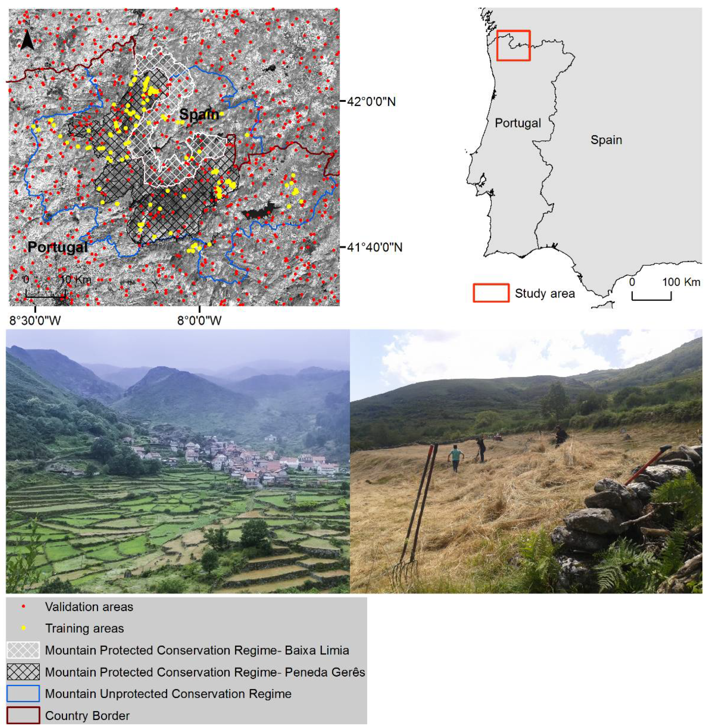
2.1. Study Area
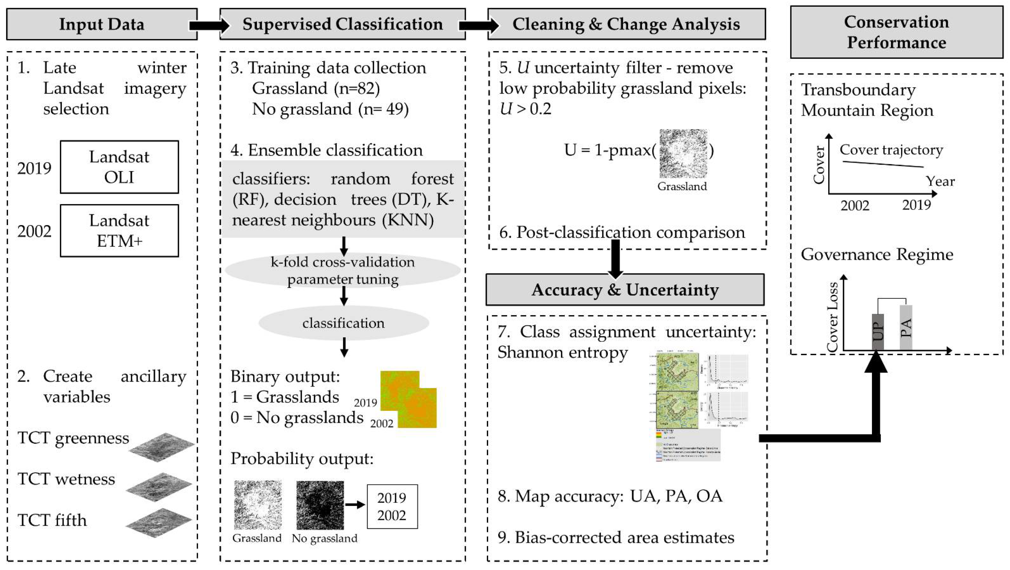
2.2. Workflow
2.2.1. Landsat Imagery and Ancillary Derivatives
2.2.2. Supervised Classification of Grassland Cover
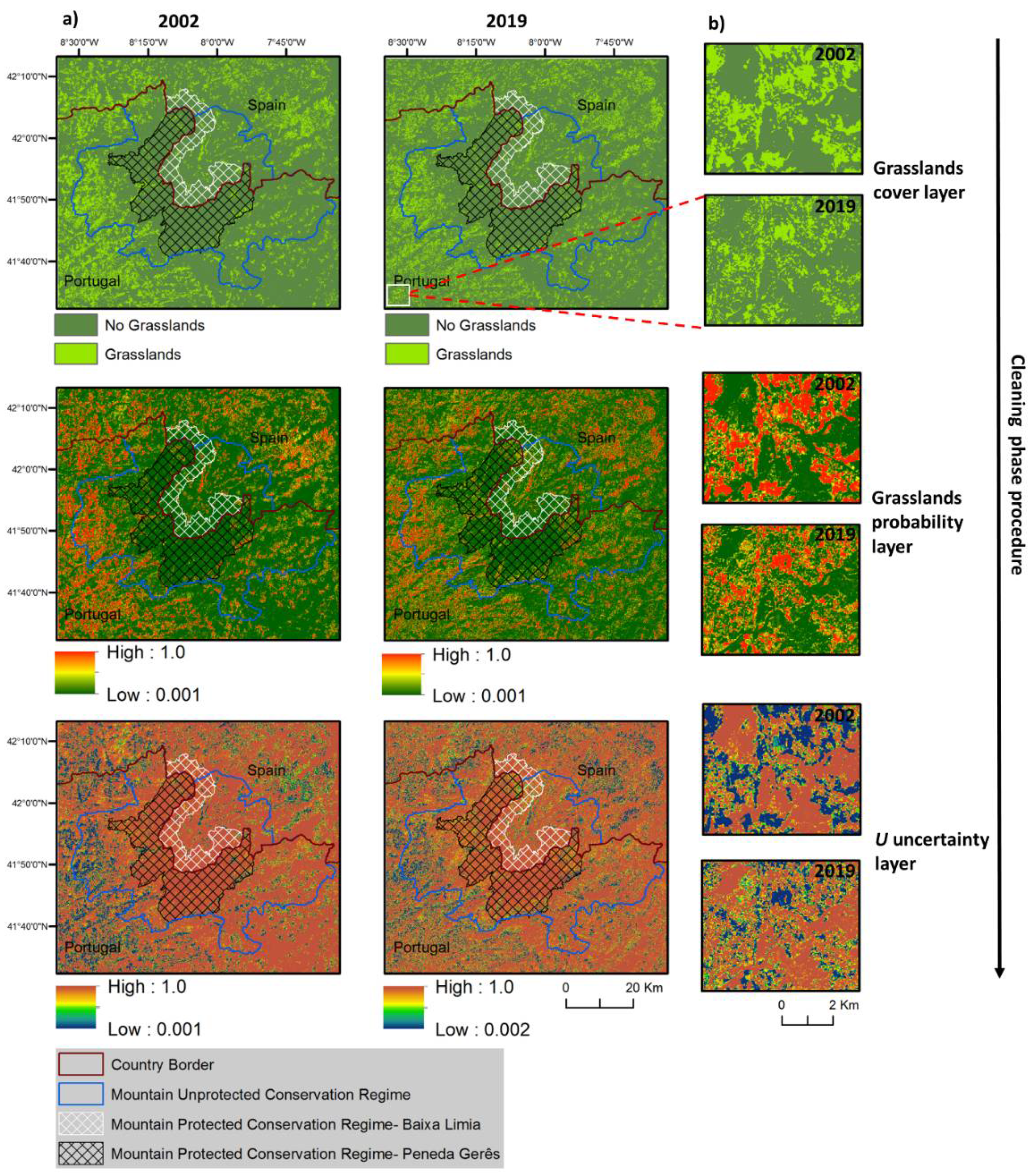
2.2.3. Cleaning Phase and Map of Grasslands Cover Change
2.2.4. Accuracy and Uncertainty Assessment: Pixel Class Assignment and Estimation of Bias-Corrected Grasslands Cover Change Areas
2.3. Statistical Analysis
3. Results
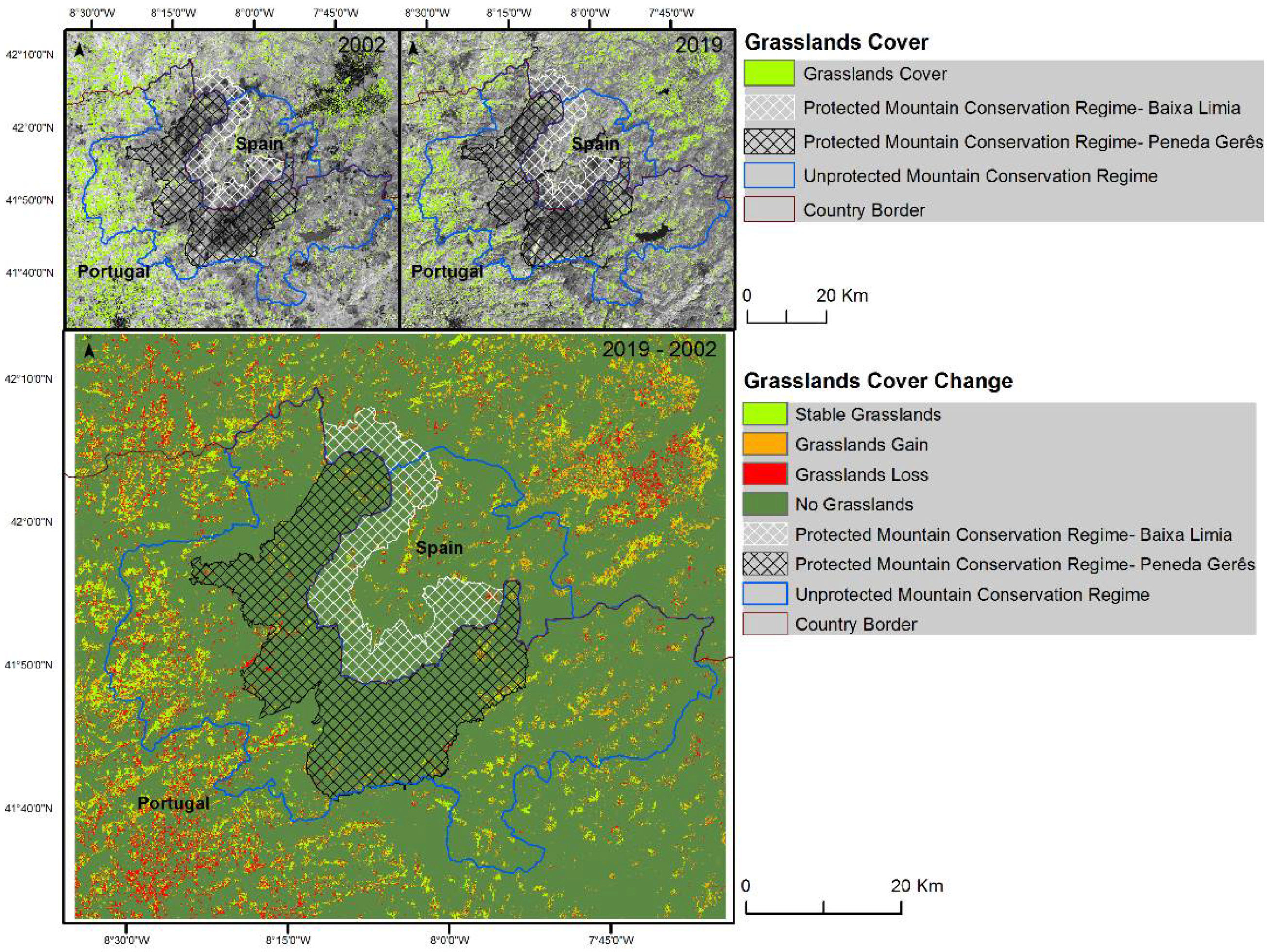
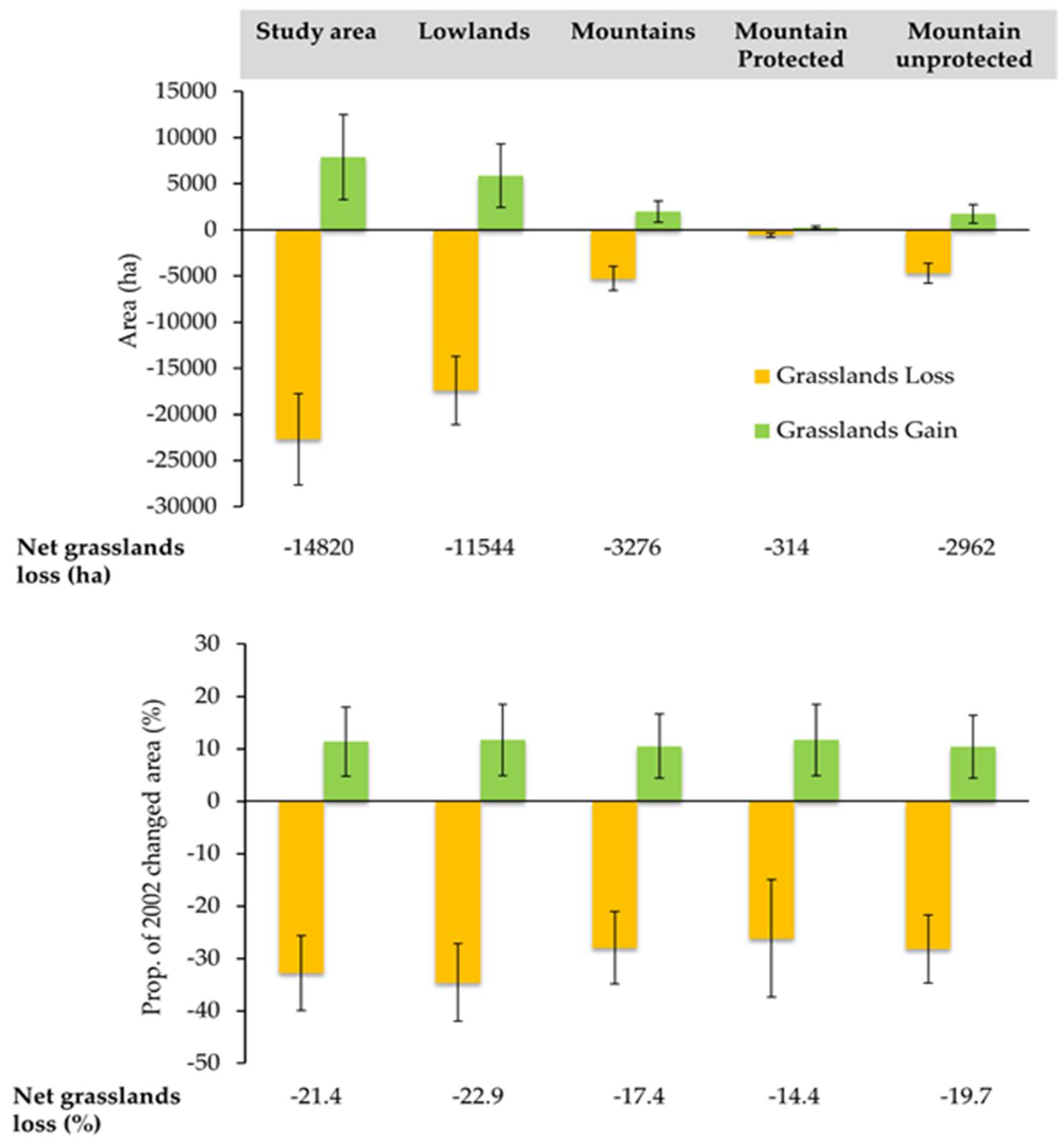
3.1. Grassland Cover Change in the Peneda-Gerês Transboundary Mountain Region
3.2. The Progress in Mountain Grasslands Conservation by 2020 and the Difference among Land Governance Regimes
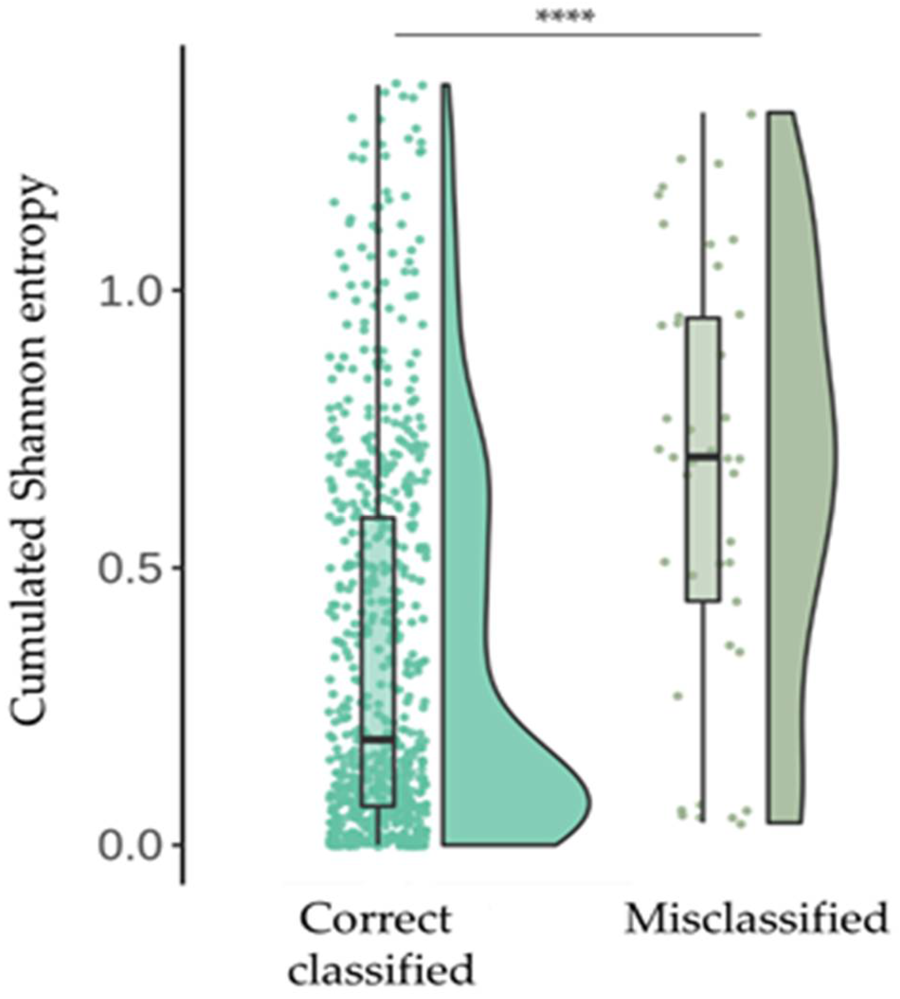
3.3. The Confidence of Grasslands Pixel Assignment and Uncertainty in Grasslands Cover Change Estimates
4. Discussion
4.1. Progress in the Conservation of Mountain Grasslands in Southern Europe by 2020
4.2. Accuracy and Uncertainty
5. Conclusions
Author Contributions
Funding
Institutional Review Board Statement
Informed Consent Statement
Data Availability Statement
Acknowledgments
Conflicts of Interest
Appendix A

| Classifier | Grid Search- Parameters Tuning | Parameterization |
|---|---|---|
| Random forest (RF) | ‘n_estimators’: [100, 300, 500, 800, 1000], ‘max_depth’:[4, 8, 16,24], ‘min_samples_leaf’:[1,2,4], ‘min_samples_split’:[2,4,6],‘criterion’: [‘gini’, ‘entropy’], ‘bootstrap’: [True, False], | n-estimators:500, criterion= ‘gini’, max_features= ‘auto’, max_depth=3, min_smaples_split=2, min_samples_leaf=1, oob_score=TRUE |
| Decision trees (DT) | ‘max_depth’:[4, 8, 16, 24], ‘min_samples_leaf’:[1,2,3,4], ‘min_samples_split’:[2,4,6], ‘criterion’: [‘gini’, ‘entropy’] | criterion= ‘gini, random_state=100, max_depth=3, min_samples_leaf=3, min_smaples_split=2, splitter=”best” |
| K-nearest neighbor (KNN) | ‘n_neighbors’:[3, 4, 5, 6], ‘leaf_size’:[1,3,5], ‘weights’: [‘distance’, ‘uniform’] | n_neighbors=3, weights=‘distance’ |
| Ensemble | Estimators= ‘RF, DT, KNN’, voting= ‘soft’ |
Appendix B
| Study Area | Reference categories | |||||||
| Map categories | No grasslands | Stable grasslands | Grasslands gain | Grasslands loss | Total | Am,i (ha) | wi | |
| No grasslands | 601 | 5 | 0 | 1 | 607 | 546995.2 | 0.86 | |
| Stable grasslands | 6 | 36 | 0 | 0 | 42 | 37712.6 | 0.06 | |
| Grasslands gain | 10 | 7 | 7 | 1 | 25 | 22149.9 | 0.03 | |
| Grasslands loss | 3 | 4 | 2 | 25 | 34 | 28434.3 | 0.04 | |
| Total | 620 | 52 | 9 | 27 | 708 | |||
| Lowlands | Reference categories | |||||||
| Map categories | No grasslands | Stable grasslands | Grasslands gain | Grasslands loss | Total | Am,i (ha) | wi | |
| No grasslands | 601 | 5 | 0 | 1 | 607 | 310314.9 | 0.83 | |
| Stable grasslands | 6 | 36 | 0 | 0 | 42 | 26959.7 | 0.07 | |
| Grasslands gain | 10 | 7 | 7 | 1 | 25 | 16367.9 | 0.04 | |
| Grasslands loss | 3 | 4 | 2 | 25 | 34 | 22116.1 | 0.06 | |
| Total | 620 | 52 | 9 | 27 | 708 | |||
| Mountains | Reference categories | |||||||
| Map categories | No grasslands | Stable grasslands | Grasslands gain | Grasslands loss | Total | Am,i (ha) | wi | |
| No grasslands | 601 | 5 | 0 | 1 | 607 | 236680.2 | 0.91 | |
| Stable grasslands | 6 | 36 | 0 | 0 | 42 | 10752.9 | 0.04 | |
| Grasslands gain | 10 | 7 | 7 | 1 | 25 | 5782.1 | 0.02 | |
| Grasslands loss | 3 | 4 | 2 | 25 | 34 | 6318.3 | 0.02 | |
| Total | 620 | 52 | 9 | 27 | 708 | |||
| Mountain Protected | Reference categories | |||||||
| Map categories | No grasslands | Stable grasslands | Grasslands gain | Grasslands loss | Total | Am,i (ha) | wi | |
| No grasslands | 601 | 5 | 0 | 1 | 607 | 67344.6 | 0.97 | |
| Stable grasslands | 6 | 36 | 0 | 0 | 42 | 884.1 | 0.01 | |
| Grasslands gain | 10 | 7 | 7 | 1 | 25 | 791.7 | 0.01 | |
| Grasslands loss | 3 | 4 | 2 | 25 | 34 | 581.6 | 0.01 | |
| Total | 620 | 52 | 9 | 27 | 708 | |||
| Mountain Unprotected | Reference categories | |||||||
| Map categories | No grasslands | Stable grasslands | Grasslands gain | Grasslands loss | Total | Am,i (ha) | wi | |
| No grasslands | 601 | 5 | 0 | 1 | 607 | 169335.3 | 0.89 | |
| Stable grasslands | 6 | 36 | 0 | 0 | 42 | 9868.9 | 0.52 | |
| Grasslands gain | 10 | 7 | 7 | 1 | 25 | 4990.3 | 0.02 | |
| Grasslands loss | 3 | 4 | 2 | 25 | 34 | 5736.7 | 0.03 | |
| Total | 620 | 52 | 9 | 27 | 708 | |||
References
- Sühs, R.B.; Giehl, E.L.H.; Peroni, N. Preventing traditional management can cause grassland loss within 30 years in southern Brazil. Sci. Rep. 2020, 10, 783. [Google Scholar] [CrossRef] [PubMed]
- Fischer, J.; Hartel, T.; Kuemmerle, T. Conservation policy in traditional farming landscapes. Conserv. Lett. 2012, 5, 167–175. [Google Scholar] [CrossRef] [Green Version]
- Schirpke, U.; Kohler, M.; Leitinger, G.; Fontana, V.; Tasser, E.; Tappeiner, U. Future impacts of changing land-use and climate on ecosystem services of mountain grassland and their resilience. Ecosyst. Serv. 2017, 26, 79–94. [Google Scholar] [CrossRef] [PubMed]
- Spiegelberger, T.; Matthies, D.; Müller-Schärer, H.; Schaffner, U. Scale-dependent effects of land use on plant species richness of mountain grassland in the European Alps. Ecography 2006, 29, 541–548. [Google Scholar] [CrossRef]
- Gartzia, M.; Fillat, F.; Pérez-Cabello, F.; Alados, C.L. Influence of Agropastoral System Components on Mountain Grassland Vulnerability Estimated by Connectivity Loss. PLoS ONE 2016, 11, e0155193. [Google Scholar] [CrossRef]
- Lavorel, S.; Grigulis, K.; Leitinger, G.; Kohler, M.; Schirpke, U.; Tappeiner, U. Historical trajectories in land use pattern and grassland ecosystem services in two European alpine landscapes. Reg. Environ. Chang. 2017, 17, 2251–2264. [Google Scholar] [CrossRef] [PubMed]
- Grau, H.R.; Aide, M. Globalization and Land-Use Transitions in Latin America. Ecol. Soc. 2008, 13. [Google Scholar] [CrossRef] [Green Version]
- European Comission, DG Environment. LIFE and Europe´s Grasslands: Restoring a Forgotten Habitat; LIFE III; European Union: Luxembourg, 2008. [Google Scholar]
- Lakner, S.; Zinngrebe, Y.; Koemle, D. Combining management plans and payment schemes for targeted grassland conservation within the Habitats Directive in Saxony, Eastern Germany. Land Use Policy 2020, 97, 104642. [Google Scholar] [CrossRef]
- Diversity, C.O.B. Decision adopted by the conference of the parties to the convention on biological diversity at its tenth meeting. Decision x/2. The strategic plan for biodiversity 2011–2020 and the aichi biodiversity targets. unep/cbd/cop/dec/x/, Ed. 2010. Nagoya, Japan, 18–29 October 2010. 29 October.
- Hinojosa, L.; Napoléone, C.; Moulery, M.; Lambin, E.F. The “mountain effect” in the abandonment of grasslands: Insights from the French Southern Alps. Agric. Ecosyst. Environ. 2016, 221, 115–124. [Google Scholar] [CrossRef]
- Hinojosa, L.; Tasser, E.; Rüdisser, J.; Leitinger, G.; Schermer, M.; Lambin, E.F.; Tappeiner, U. Geographical heterogeneity in mountain grasslands dynamics in the Austrian-Italian Tyrol region. Appl. Geogr. 2019, 106, 50–59. [Google Scholar] [CrossRef]
- Regos, A.; Ninyerola, M.; Moré, G.; Pons, X. Linking land cover dynamics with driving forces in mountain landscape of the Northwestern Iberian Peninsula. Int. J. Appl. Earth Obs. Geoinf. 2015, 38, 1–14. [Google Scholar] [CrossRef]
- Aune, S.; Bryn, A.; Hovstad, K.A. Loss of semi-natural grassland in a boreal landscape: Impacts of agricultural intensification and abandonment. J. Land Use Sci. 2018, 13, 375–390. [Google Scholar] [CrossRef]
- Halada, Ľ.; David, S.; Hreško, J.; Klimantová, A.; Bača, A.; Rusňák, T.; Buraľ, M.; Vadel, Ľ. Changes in grassland management and plant diversity in a marginal region of the Carpathian Mts. in 1999–2015. Sci. Total Environ. 2017, 609, 896–905. [Google Scholar] [CrossRef] [PubMed]
- Jaworek-Jakubska, J.; Filipiak, M.; Napierała-Filipiak, A. Understanding of Forest Cover Dynamics in Traditional Landscapes: Mapping Trajectories of Changes in Mountain Territories (1824–2016), on the Example of Jeleniogórska Basin, Poland. Forests 2020, 11, 867. [Google Scholar] [CrossRef]
- Malavasi, M.; Carranza, M.L.; Moravec, D.; Cutini, M. Reforestation dynamics after land abandonment: A trajectory analysis in Mediterranean mountain landscapes. Reg. Environ. Chang. 2018, 18, 2459–2469. [Google Scholar] [CrossRef]
- Geldmann, J.; Manica, A.; Burgess, N.D.; Coad, L.; Balmford, A. A global-level assessment of the effectiveness of protected areas at resisting anthropogenic pressures. Proc. Natl. Acad. Sci. USA 2019, 116, 23209–23215. [Google Scholar] [CrossRef] [PubMed]
- Chape, S.; Harrison, J.; Spalding, M.; Lysenko, I. Measuring the extent and effectiveness of protected areas as an indicator for meeting global biodiversity targets. Philos. Trans. R. Soc. B Biol. Sci. 2005, 360, 443–455. [Google Scholar] [CrossRef] [Green Version]
- Ridding, L.E.; Redhead, J.W.; Pywell, R.F. Fate of semi-natural grassland in England between 1960 and 2013: A test of national conservation policy. Glob. Ecol. Conserv. 2015, 4, 516–525. [Google Scholar] [CrossRef] [Green Version]
- Huang, C.; Wylie, B.; Yang, L.; Homer, C.; Zylstra, G. Derivation of a tasselled cap transformation based on Landsat 7 at-satellite reflectance. Int. J. Remote Sens. 2002, 23, 1741–1748. [Google Scholar] [CrossRef]
- Olofsson, P.; Foody, G.M.; Herold, M.; Stehman, S.V.; Woodcock, C.E.; Wulder, M.A. Good practices for estimating area and assessing accuracy of land change. Remote Sens. Environ. 2014, 148, 42–57. [Google Scholar] [CrossRef]
- Schleicher, J.; Peres, C.A.; Leader-Williams, N. Conservation performance of tropical protected areas: How important is management? Conserv. Lett. 2019, 12, e12650. [Google Scholar] [CrossRef] [Green Version]
- Leite, A.; Cáceres, A.; Melo, M.; Mills, M.S.L.; Monteiro, A.T. Reducing emissions from Deforestation and forest Degradation in Angola: Insights from the scarp forest conservation ‘hotspot’. Land Degrad. Dev. 2018, 29, 4291–4300. [Google Scholar] [CrossRef]
- Ali, I.; Cawkwell, F.; Dwyer, E.; Barrett, B.; Green, S. Satellite remote sensing of grasslands: From observation to management. J. Plant. Ecol. 2016, 9, 649–671. [Google Scholar] [CrossRef] [Green Version]
- Tarantino, C.; Adamo, M.; Lucas, R.; Blonda, P. Detection of changes in semi-natural grasslands by cross correlation analysis with WorldView-2 images and new Landsat 8 data. Remote Sens. Environ. 2016, 175, 65–72. [Google Scholar] [CrossRef]
- Lopes, M.; Fauvel, M.; Girard, S.; Sheeren, D. Object-Based Classification of Grasslands from High Resolution Satellite Image Time Series Using Gaussian Mean Map Kernels. Remote Sens. 2017, 9, 688. [Google Scholar] [CrossRef] [Green Version]
- Lei, G.; Li, A.; Bian, J.; Yan, H.; Zhang, L.; Zhang, Z.; Nan, X. OIC-MCE: A Practical Land Cover Mapping Approach for Limited Samples Based on Multiple Classifier Ensemble and Iterative Classification. Remote Sens. 2020, 12, 987. [Google Scholar] [CrossRef] [Green Version]
- Shen, H.; Lin, Y.; Tian, Q.; Xu, K.; Jiao, J. A comparison of multiple classifier combinations using different voting-weights for remote sensing image classification. Int. J. Remote Sens. 2018, 39, 3705–3722. [Google Scholar] [CrossRef]
- Loosvelt, L.; Peters, J.; Skriver, H.; Lievens, H.; Van Coillie, F.M.B.; De Baets, B.; Verhoest, N.E.C. Random Forests as a tool for estimating uncertainty at pixel-level in SAR image classification. Int. J. Appl. Earth Obs. Geoinf. 2012, 19, 173–184. [Google Scholar] [CrossRef]
- Vaz, A.S.; Marcos, B.; Gonçalves, J.; Monteiro, A.; Alves, P.; Civantos, E.; Lucas, R.; Mairota, P.; Garcia-Robles, J.; Alonso, J.; et al. Can we predict habitat quality from space? A multi-indicator assessment based on an automated knowledge-driven system. Int. J. Appl. Earth Obs. Geoinf. 2015, 37, 106–113. [Google Scholar] [CrossRef]
- Panuju, D.R.; Paull, D.J.; Griffin, A.L. Change Detection Techniques Based on Multispectral Images for Investigating Land Cover Dynamics. Remote Sens. 2020, 12, 1781. [Google Scholar] [CrossRef]
- Schott, J.R.; Salvaggio, C.; Volchok, W.J. Radiometric scene normalization using pseudoinvariant features. Remote Sens. Environ. 1988, 26, 1–16. [Google Scholar] [CrossRef]
- Baig, M.H.A.; Zhang, L.; Shuai, T.; Tong, Q. Derivation of a tasselled cap transformation based on Landsat 8 at-satellite reflectance. Remote Sens. Lett. 2014, 5, 423–431. [Google Scholar] [CrossRef]
- Kloucek, T.; Moravec, D.; Komarek, J.; Lagner, O.; Stych, P. Selecting appropriate variables for detecting grassland to cropland changes using high resolution satellite data. PeerJ 2018, 6, e5487. [Google Scholar] [CrossRef] [PubMed]
- Google Earth. Peneda-Gerês, Portugal. 41°42’59” N, −8°08’60” W. Google. Available online: https://earth.google.com/web/@41.8801128,-8.220861,532.51768276a,1674.6551658d,35y,27.84655945h,59.98928978t,-0r/data=Cl0aWxJVCiQweGQyNTE0MGM3M2NjNzJiMToweDY4MjBiNDY1NjM0YjNlOTcZTe4cb5fwREAhP-QtVz9uIMAqG1NvYWpvTmF0dXJlIC0gUGVuZWRhIEdlcsOqcxgBIAE (accessed on 19 November 2020).
- Jozdani, S.E.; Johnson, B.A.; Chen, D. Comparing Deep Neural Networks, Ensemble Classifiers, and Support Vector Machine Algorithms for Object-Based Urban Land Use/Land Cover Classification. Remote Sens. 2019, 11, 1713. [Google Scholar] [CrossRef] [Green Version]
- Contributors, G.O. GDAL/OGR Geospatial Data Abstraction Software Library; Open Source Geospatial Foundation: Beaverton, OR, USA, 2020. [Google Scholar]
- Pedregosa, F.; Varoquaux, G.; Gramfort, A.; Michel, V.; Thirion, B.; Grisel, O.; Blondel, M.; Prettenhofer, P.; Weiss, R.; Dubourg, V.; et al. Scikit-learn: Machine Learning in Python. JMLR J. Mach. Learn. Res. 2011, 12, 2825–2830. [Google Scholar]
- Leadley, P.W.; Krug, C.B.; Alkemade, R.; Pereira, H.M.; Sumaila, U.R.; Walpole, M.; Marques, A.; Newbold, T.; Teh, L.S.L.; van Kolck, J.; et al. Progress towards the Aichi Biodiversity Targets: An. Assessment of Biodiversity Trends, Policy Scenarios and Key Actions; CBD technical series nº 78; Secretariat of the Convention on Biological Diversity: Montreal, QC, Canada, 2014. [Google Scholar]
- Shannon, C.E. A Mathematical Theory of Communication. Bell Syst. Tech. J. 1948, 27, 379–423. [Google Scholar] [CrossRef] [Green Version]
- Hothorn, T.; Hornik, K.; van de Wiel, M.A.; Zeileis, A. Implementing a Class of Permutation Tests: The coin Package. J. Stat. Softw. 2008, 28, 23. [Google Scholar] [CrossRef]
- Fava, F.; Parolo, G.; Colombo, R.; Gusmeroli, F.; Della Marianna, G.; Monteiro, A.T.; Bocchi, S. Fine-scale assessment of hay meadow productivity and plant diversity in the European Alps using field spectrometric data. Agric. Ecosyst. Environ. 2010, 137, 151–157. [Google Scholar] [CrossRef]
- Monteiro, A.T.; Fava, F.; Hiltbrunner, E.; Della Marianna, G.; Bocchi, S. Assessment of land cover changes and spatial drivers behind loss of permanent meadows in the lowlands of Italian Alps. Landsc. Urban. Plan. 2011, 100, 287–294. [Google Scholar] [CrossRef]
- García-Llamas, P.; Geijzendorffer, I.R.; García-Nieto, A.P.; Calvo, L.; Suárez-Seoane, S.; Cramer, W. Impact of land cover change on ecosystem service supply in mountain systems: A case study in the Cantabrian Mountains (NW of Spain). Reg. Environ. Chang. 2019, 19, 529–542. [Google Scholar] [CrossRef]
- Rutz, C.; Dwyer, J.; Schramek, J. More New Wine in the Same Old Bottles? The Evolving Nature of the CAP Reform Debate in Europe, and Prospects for the Future. Sociol. Rural. 2014, 54, 266–284. [Google Scholar] [CrossRef] [Green Version]
- Plieninger, T.; Hui, C.; Gaertner, M.; Huntsinger, L. The impact of land abandonment on species richness and abundance in the Mediterranean Basin: A meta-analysis. PLoS ONE 2014, 9, e98355. [Google Scholar] [CrossRef]
- Sil, Â.; Fernandes, P.M.; Rodrigues, A.P.; Alonso, J.M.; Honrado, J.P.; Perera, A.; Azevedo, J.C. Farmland abandonment decreases the fire regulation capacity and the fire protection ecosystem service in mountain landscapes. Ecosyst. Serv. 2019, 36, 100908. [Google Scholar] [CrossRef] [Green Version]
- Speed, J.D.M.; Austrheim, G.; Birks, H.J.B.; Johnson, S.; Kvamme, M.; Nagy, L.; Sjögren, P.; Skar, B.; Stone, D.; Svensson, E.; et al. Natural and cultural heritage in mountain landscapes: Towards an integrated valuation. Int. J. Biodivers. Sci. Ecosyst. Serv. Manag. 2012, 8, 313–320. [Google Scholar] [CrossRef] [Green Version]
- Jäger, H.; Peratoner, G.; Tappeiner, U.; Tasser, E. Grassland biomass balance in the European Alps: Current and future ecosystem service perspectives. Ecosyst. Serv. 2020, 45, 101163. [Google Scholar] [CrossRef]
- Perpiña Castillo, C.; Coll Aliaga, E.; Lavalle, C.; Martínez Llario, J.C. An Assessment and Spatial Modelling of Agricultural Land Abandonment in Spain (2015–2030). Sustainability 2020, 12, 560. [Google Scholar] [CrossRef] [Green Version]
- Ribas, L.G.d.S.; Pressey, R.L.; Loyola, R.; Bini, L.M. A global comparative analysis of impact evaluation methods in estimating the effectiveness of protected areas. Biol. Conserv. 2020, 246, 108595. [Google Scholar] [CrossRef]
- Dengler, J.; Tischew, S. Grasslands of western and northern Europe—Between intensification and abandonment. In Grasslands of the World: Diversity, Management and Conservation; Squires, V.R., Dengler, J., Hua, L., Feng, H., Eds.; CRC Press: Boca Raton, FL, USA, 2018. [Google Scholar]
- Lopes, M.; Fauvel, M.; Ouin, A.; Girard, S. Spectro-Temporal Heterogeneity Measures from Dense High Spatial Resolution Satellite Image Time Series: Application to Grassland Species Diversity Estimation. Remote Sens. 2017, 9, 993. [Google Scholar] [CrossRef] [Green Version]
- Pôças, I.; Cunha, M.; Pereira, L.S. Remote sensing based indicators of changes in a mountain rural landscape of Northeast Portugal. Appl. Geogr. 2011, 31, 871–880. [Google Scholar] [CrossRef]
- Griffiths, P.; Müller, D.; Kuemmerle, T.; Hostert, P. Agricultural land change in the Carpathian ecoregion after the breakdown of socialism and expansion of the European Union. Environ. Res. Lett. 2013, 8, 045024. [Google Scholar] [CrossRef]
- Toivonen, T.; Luoto, M. Landsat TM images in mapping of semi-natural grasslands and analysing of habitat pattern in an agricultural landscape in south-west Finland. Fenn. Int. J. Geogr. 2003, 181, 49–67. [Google Scholar]
- Khatami, R.; Mountrakis, G.; Stehman, S.V. Mapping per-pixel predicted accuracy of classified remote sensing images. Remote Sens. Environ. 2017, 191, 156–167. [Google Scholar] [CrossRef] [Green Version]


| Classification | Reference Training Data | |||
|---|---|---|---|---|
| Method | Classifier Parameterization | Class | Training Sites | N° of Pixels |
| Multiple Classifier Ensemble (MCE) | Random Forests (n_estimators = 500, criterion = ‘gini’, max_depth = 4, min_samples_split= 2, min_samples_leaf = 1, max_features = ‘auto’, bootstrap = True, oob_score = True); Decision Trees (criterion = ‘entropy’, max_depth = 4, min_samples_leaf = 1, min_samples_split = 2, random_state = 100); K-nearest neighbors (n_neighbors = 4, weights = ‘distance’, leaf_size = 1); | Grasslands | 82 | 272 |
| No Grasslands | 49 | 579 | ||
| Total | 131 | 851 | ||
| Period (2019–2002) | Mapped Area (ha) | Bias-Corrected (ha) | Standard Error of Bias-Corrected Area Estimate (ha) | Confidence Interval (95%; ha) | ||||
|---|---|---|---|---|---|---|---|---|
| Stable Grasslands | No Grasslands | Stable Grasslands | No Grasslands | Stable Grasslands | No Grasslands | Stable Grasslands | No Grasslands | |
| Study area | 37713 | 546995 | 46378 | 558345 | 3866 | 3995 | 7577 | 7829 |
| Lowlands | 26959 | 310315 | 32849 | 319598 | 2694 | 2756 | 5280 | 5402 |
| Mountains | 10752.9 | 236680 | 13259 | 238747 | 1228 | 1297 | 2406 | 2542 |
| Mountain protected | 885 | 67345 | 1603 | 67173 | 264 | 288 | 518 | 564 |
| Mountain unprotected | 9869 | 169335 | 11926 | 171574 | 995 | 1041 | 1950 | 2040 |
| Extent of Analysis | Grasslands Cover (ha) | Sample Size (ha) | Pearson’s Chi-Squared (X2) | P (Two-Tailed) | |
|---|---|---|---|---|---|
| Year 2019 | Year 2002 | ||||
| Study area | 58159 | 72401 | 635292 | 1972.1 | p < 0.001 |
| Lowlands | 38733 | 50277 | 375759 | 1698 | p < 0.001 |
| Mountains | 15519 | 18796 | 259533 | 334.9 | p < 0.001 |
| Mountains protected | 1859 | 2173 | 69602 | 25 | p < 0.001 |
| Mountains unprotected | 13661 | 16623 | 189932 | 314.6 | p < 0.001 |
| Grasslands Net Loss (ha) | Sample Size (ha) | Pearson’s Chi-Squared (X2) | P (Two-Tailed) | ||
| Mountains protected | 314 | 2173 | 14.9 | p < 0.001 | |
| Mountains unprotected | 2962 | 16623 | |||
| Study Area | Reference categories | |||||||||
| Map categories | No grasslands | Stable grasslands | Grasslands gain | Grasslands loss | Total | Wi | User’s | Producer’s | Overall | |
| No grasslands | 0.853 | 0.007 | 0.000 | 0.001 | 607 | 0.86 | 0.99 | 0.97 | 0.95 ± 0.02 | |
| Stable grasslands | 0.008 | 0.051 | 0.000 | 0.000 | 42 | 0.06 | 0.86 | 0.70 | ||
| Grasslands gain | 0.014 | 0.010 | 0.010 | 0.001 | 25 | 0.03 | 0.28 | 0.79 | ||
| Grasslands loss | 0.004 | 0.005 | 0.003 | 0.033 | 34 | 0.04 | 0.74 | 0.92 | ||
| Total | 0.879 | 0.073 | 0.012 | 0.036 | 708 | 1.00 | ||||
| Lowlands | Reference categories | |||||||||
| Map categories | No grasslands | Stable grasslands | Grasslands gain | Grasslands loss | Total | Wi | User’s | Producer’s | Overall | |
| No grasslands | 0.818 | 0.007 | 0.000 | 0.001 | 607 | 0.826 | 0.99 | 0.96 | 0.93 ± 0.02 | |
| Stable grasslands | 0.010 | 0.061 | 0.000 | 0.000 | 42 | 0.072 | 0.86 | 0.70 | ||
| Grasslands gain | 0.017 | 0.012 | 0.012 | 0.002 | 25 | 0.044 | 0.28 | 0.78 | ||
| Grasslands loss | 0.005 | 0.007 | 0.003 | 0.043 | 34 | 0.059 | 0.74 | 0.93 | ||
| Total | 0.851 | 0.087 | 0.016 | 0.046 | 708 | 1.00 | ||||
| Mountains | Reference categories | |||||||||
| Map categories | No grasslands | Stable grasslands | Grasslands gain | Grasslands loss | Total | Wi | User’s | Producer’s | Overall | |
| No grasslands | 0.903 | 0.008 | 0.000 | 0.002 | 607 | 0.912 | 0.98 | 0.98 | 0.96 ± 0.01 | |
| Stable grasslands | 0.006 | 0.036 | 0.000 | 0.000 | 42 | 0.041 | 0.86 | 0.68 | ||
| Grasslands gain | 0.009 | 0.006 | 0.006 | 0.001 | 25 | 0.022 | 0.28 | 0.81 | ||
| Grasslands loss | 0.002 | 0.003 | 0.001 | 0.018 | 34 | 0.024 | 0.74 | 0.88 | ||
| Total | 0.92 | 0.052 | 0.008 | 0.002 | 708 | 1.00 | ||||
| Mountain Protected | Reference categories | |||||||||
| Map categories | No grasslands | Stable grasslands | Grasslands gain | Grasslands loss | Total | Wi | User’s | Producer’s | Overall | |
| No grasslands | 0.958 | 0.008 | 0.000 | 0.002 | 607 | 0.968 | 0.99 | 0.99 | 0.97 ± 0.01 | |
| Stable grasslands | 0.002 | 0.011 | 0.000 | 0.000 | 42 | 0.013 | 0.86 | 0.47 | ||
| Grasslands gain | 0.005 | 0.003 | 0.003 | 0.000 | 25 | 0.011 | 0.28 | 0.87 | ||
| Grasslands loss | 0.001 | 0.001 | 0.001 | 0.006 | 34 | 0.008 | 0.74 | 0.75 | ||
| Total | 0.965 | 0.023 | 0.004 | 0.008 | 708 | 1.00 | ||||
| Mountain Unprotected | Reference categories | |||||||||
| Map categories | No grasslands | Stable grasslands | Grasslands gain | Grasslands loss | Total | Wi | User’s | Producer’s | Overall | |
| No grasslands | 0.883 | 0.007 | 0.000 | 0.001 | 607 | 0.892 | 0.99 | 0.99 | 0.96 ± 0.01 | |
| Stable grasslands | 0.007 | 0.045 | 0.000 | 0.000 | 42 | 0.052 | 0.86 | 0.71 | ||
| Grasslands gain | 0.011 | 0.007 | 0.007 | 0.000 | 25 | 0.026 | 0.28 | 0.81 | ||
| Grasslands loss | 0.003 | 0.004 | 0.002 | 0.022 | 34 | 0.030 | 0.74 | 0.90 | ||
| Total | 0.903 | 0.063 | 0.009 | 0.025 | 708 | 1.00 | ||||
Publisher’s Note: MDPI stays neutral with regard to jurisdictional claims in published maps and institutional affiliations. |
© 2021 by the authors. Licensee MDPI, Basel, Switzerland. This article is an open access article distributed under the terms and conditions of the Creative Commons Attribution (CC BY) license (https://creativecommons.org/licenses/by/4.0/).
Share and Cite
Monteiro, A.T.; Carvalho-Santos, C.; Lucas, R.; Rocha, J.; Costa, N.; Giamberini, M.; Costa, E.M.d.; Fava, F. Progress in Grassland Cover Conservation in Southern European Mountains by 2020: A Transboundary Assessment in the Iberian Peninsula with Satellite Observations (2002–2019). Remote Sens. 2021, 13, 3019. https://doi.org/10.3390/rs13153019
Monteiro AT, Carvalho-Santos C, Lucas R, Rocha J, Costa N, Giamberini M, Costa EMd, Fava F. Progress in Grassland Cover Conservation in Southern European Mountains by 2020: A Transboundary Assessment in the Iberian Peninsula with Satellite Observations (2002–2019). Remote Sensing. 2021; 13(15):3019. https://doi.org/10.3390/rs13153019
Chicago/Turabian StyleMonteiro, Antonio T., Cláudia Carvalho-Santos, Richard Lucas, Jorge Rocha, Nuno Costa, Mariasilvia Giamberini, Eduarda Marques da Costa, and Francesco Fava. 2021. "Progress in Grassland Cover Conservation in Southern European Mountains by 2020: A Transboundary Assessment in the Iberian Peninsula with Satellite Observations (2002–2019)" Remote Sensing 13, no. 15: 3019. https://doi.org/10.3390/rs13153019