Article

Semantic Boosting: Enhancing Deep Learning Based LULC Classification

by
Marvin Mc Cutchan
1,2,*,
Alexis J. Comber
3,
Ioannis Giannopoulos
1,2 and
Manuela Canestrini
1
1
Department of Geodesy and Geoinformation, TU Wien, 1040 Vienna, Austria
2
Institute of Advanced Research in Artificial Intelligence (IARAI), 1030 Vienna, Austria
3
Leeds Institute for Data Analytics, University of Leeds, Leeds LS2 9NL, UK
*
Author to whom correspondence should be addressed.
Remote Sens. 2021, 13(16), 3197; https://doi.org/10.3390/rs13163197
Submission received: 26 July 2021 / Revised: 6 August 2021 / Accepted: 8 August 2021 / Published: 12 August 2021

Abstract

:
The classification of land use and land cover (LULC) is a well-studied task within the domain of remote sensing and geographic information science. It traditionally relies on remotely sensed imagery and therefore models land cover classes with respect to their electromagnetic reflectances, aggregated in pixels. This paper introduces a methodology which enables the inclusion of geographical object semantics (from vector data) into the LULC classification procedure. As such, information on the types of geographic objects (e.g., Shop, Church, Peak, etc.) can improve LULC classification accuracy. In this paper, we demonstrate how semantics can be fused with imagery to classify LULC. Three experiments were performed to explore and highlight the impact and potential of semantics for this task. In each experiment CORINE LULC data was used as a ground truth and predicted using imagery from Sentinel-2 and semantics from LinkedGeoData using deep learning. Our results reveal that LULC can be classified from semantics only and that fusing semantics with imagery—Semantic Boosting—improved the classification with significantly higher LULC accuracies. The results show that some LULC classes are better predicted using only semantics, others with just imagery, and importantly much of the improvement was due to the ability to separate similar land use classes. A number of key considerations are discussed.

1. Introduction

Land cover classes or types can be defined and determined in multiple ways. This can lead to ambiguous understandings of their characteristics and consequently their spatial distribution. Such ambiguity can arise from different mapping project objectives and the fact that different entities may view a given type of land cover differently in terms of its physical properties as well as different conceptualisations of land cover classes [1]. In addition, land cover can be modelled and determined from different data sources, the most prominent of which is remotely sensed imagery. This is commonly used to determine the presence of different land covers with respect to their electromagnetic signatures. The characteristics of this data influence how land cover is captured as a function of both the pixel [2] and pixel size [3]. Thus, any knowledge (including data) about the spatial distribution of land cover is inherently linked to how land cover classes are defined and recorded, with clear implications for applications that depend on land cover data. Uncertainty in this knowledge can have profound effects on the results of land use and land cover (LULC, as the terms are frequently used interchangably) data analyses, for example, as drivers of climate [4,5], the environment [6], on the allocation of land and resources [4,5,7], and on understanding biodiversity [8], with implications for decision making. Remotely sensed imagery allows LULC to be classified with high accuracy but only with respect to the aggregated electromagnetic reflectance as recorded in a pixel. This can exclude relevant information, such as how land is used, which is not captured by remotely sensing imagery. The aim of this work is to compensate for such limitations, by including geospatial semantics [9] into the LULC classification process. The semantics describe the types of geo-objects (e.g., House, Bench, Peak, etc.) and therefore relate to social and economic activity describing how the land is used. This paper demonstrates how geospatial semantics (which describes the land use) can be combined with imagery (which describes the land cover) in order to improve LULC classification. The contribution of this work is threefold:
(1)
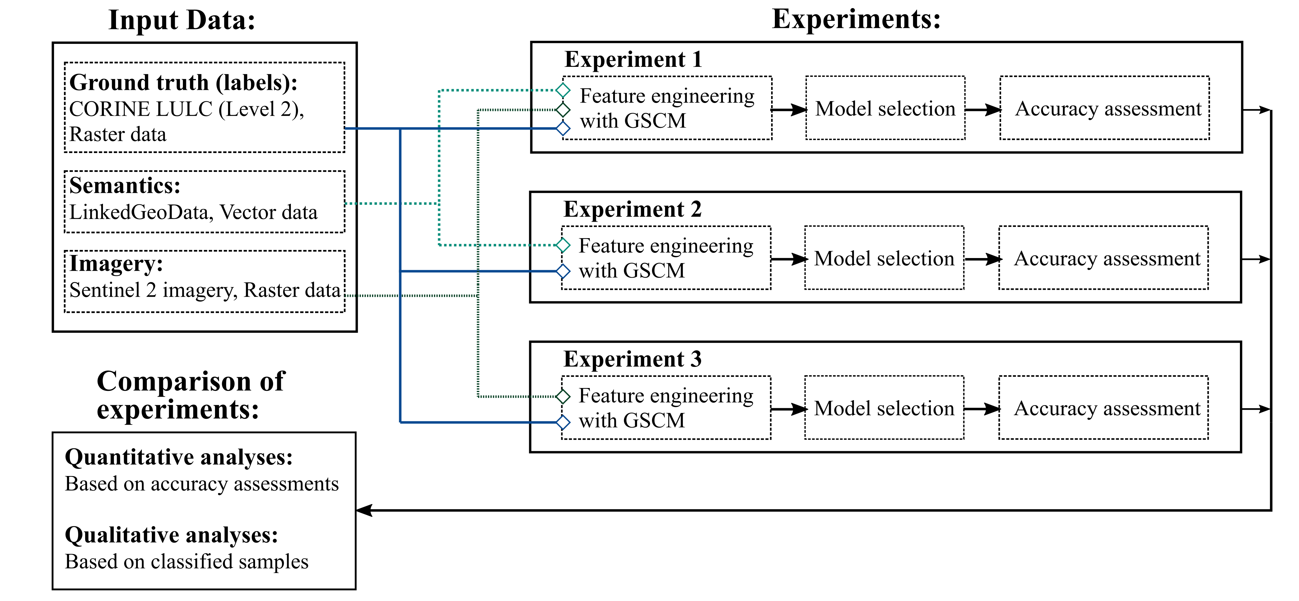
The development and application of a Semantic Boosting approach, for fusing remotely sensed imagery with geospatial semantics (obtained from vector data) for LULC classification based on deep learning;
(2)
A quantitative analysis investigating the potential of geospatial semantics for LULC classification in depth;
(3)
A qualitative analysis focusing on understanding and explaining when and why Semantic Boosting can be beneficial for LULC classification.
Similar to other work [10,11,12,13], CORINE is used here as ground truth data on LULC. The deep learning model seeks to predict the CORINE LULC class for a large area and a fusion of semantics (vector data) and imagery (raster data) is used to enhance this classification. This was compared with the results of classification from two deep learning models, one using imagery only and the other using semantics only in order to generate important insights on the characteristics of Semantic Boosting. This research utilises the following datasets covering the area of Austria, serving as a case study:
The novelty of this work is that it demonstrates the utility of including local semantic information in classifying land cover and how geospatial semantics can improve the accuracy of land cover classification in a meaningful way. Section 2 reviews related research using local ancillary information for land cover classification and some of the assumptions associated with classifying remotely sensed imagery into land cover and land use. Section 3 describes the data and methodology for fusing semantics and remotely sensed imagery for LULC classification. It also describes the experiments which were carried out in order to assess the potential of this data fusion. The results are described in Section 4, with a discussion of the findings and methods in Section 5. Finally, some conclusions are drawn in Section 6.

2. Related Work

2.1. Land Use and Land Cover Semantics

Data on land use and land cover (LULC)—the two concepts are rolled together in most classifications including CORINE as discussed below—are important. They are used to understand environmental dynamics at global [4,5,15], regional [7,8,16], and local [17] scales for natural resource management, climate change, disease spread, air quality, and other ecosystem services. Different land covers and uses are associated with specific processes. For example, urban areas (land use) with lots of artificial surfaces (land cover) can result in heat islands and increase the ozone levels [4]. Agricultural expansion (land use) can decrease the water quality and the amount of carbon dioxide stored in the landscape [4,5,7,16]. The distribution of LULC has a significant impact on the global average surface temperature and variability of the climate system [5]. Reliable land use and land cover data is important for many activities related to planning sustainable global development [18,19,20]. Furthermore, LULC change influences biodiversity [8], ecosystem services [21], carbon emissions [22], and land surface temperature [23,24]. It is modeled using LULC classification products, typically (although erroneously—see [25]) through some post classification procedures (as reviewed in [26,27]). Many LULC change models therefore depend on the quality of the initial LULC classifications.
Regional LULC products have been created, such as CORINE (LULC classification for Europe), NALCD (LULC for North America), and AFRICOVER (LULC for Africa) [28]. These products were created using different methods and different types of remotely sensed imagery. The choice, definition, and number of LULC classes will impact how the features on the ground are represented as well as influence the classification accuracy [29,30]. Accuracy is influenced by the sensor type [29], the spatial resolution of the image data [31], and the number of LULC classes (negatively correlated with overall accuracy [32]). A final observation is that different LULC products have differing levels of accuracy with global, continental, and national products having accuracies ranging from 66.9% to 98.0% [28]. Reference [28] compared different LULC products and found GeoWiki (https://www.geo-wiki.org/ accessed on 30 January 2021) to have the highest accuracy of global LULC products with 10 LULC classes and a spatial resolution of 300 m × 300 m, a South American 30 m × 30 m product with 5 classes to have overall accuracy of 89.0 and a Russian 1 km × 1 km resolution dataset with 8 classes to have the highest accuracy (98.0%) amongst national products.
LULC classification is traditionally performed based on remotely sensed imagery under two inherit assumptions. (1) that LULC processes are captured by electromagnetic reflectances and can be differentiated [33] and (2) that the world can be described as a regular tessellation, i.e., a raster [2]. Reference [33] point out that LULC classes are delineated by subspaces within a feature space defined by numerical values retrieved by the electromagnetic reflectances captured remotely. However, they note that electromagnetic signatures are not consistent for different scenes, sensors, landscape contexts, and spatial scales and that in contrast to land cover, land use cannot be defined by electromagnetic signatures in a coherent and consistent manner. This is because land cover refers to the physical material at the surface of the earth, whereas land use is characterised by how people utilise the corresponding land, and as a result land use and land cover cannot be directly inferred from each other: a single land cover can have different land uses, and a single land use may be composed of different land covers. Thus, although land cover and land use are highly intertwined concepts, they can only be partly be identified from their electromagnetic reflectance values in remotely sensed imagery. The second assumption is introduced by modelling the real world using a raster representation. In a short letter, ref. [2] unpicks the ubiquitous use of the tessellated pixel as the default mode for representing real world objects that are not pixel shaped and landscape processes that do not exhibit this regular characteristic. Additionally, Reference [34] notes that the pixel introduces a topological bias, which differs from the vector model, such that pixel representations do not correctly capture topological relationships. These assumptions can lead to inconsistencies which ultimately propagate error and can confuse the modelling of environmental processes [2].
Thus, the semantics, meaning, and concepts (and accuracy) of any LULC dataset are deeply linked to the methods used to generate the data—its epistemology [35]. This includes decisions over imagery (type, scale), how features are represented, choice of training data, and classification algorithm.

2.2. New Forms and Sources of LULC-Related Information

Next to remotely sensed data, other data sources have been used to detect LULC such as cell phone data [36], social media data [37], or, volunteered geographic information (VGI), such as OpenStreetMap (OSM), with some limitations [38,39,40,41]. Reference [38] developed a LULC product for the city of Heidelberg, Germany, by using OSM data and remotely sensed imagery (Landsat) and harmonising OSM tags with Level 2 CORINE labels. Thus, a LULC class from CORINE was defined by a set of OSM tags and empty OSM areas were filled with classified satellite imagery using a classifier trained on OSM. The resulting LULC data had an overall accuracy of 81% with significant variation in per class accuracies. In [41], imagery was combined with POI data and a raster data from a Chinese internet provider (usage per grid cell) to classify LULC. They transform the imagery into visual continuous bags of words and combine it with labels of the other two datasets (also continuous bags of words) to finally apply a latent Dirichlet allocation (LDA) and random forest classifier to determine six different LULC classes within Shenzhen, China. The overall accuracy was 85.1% with a kappa coefficient of 0.812. However, both [38,41] restrict their work to one specific ROI, as a result failing to show how their approach generalises in areas with different image signatures and contexts such as rural areas, mountainous areas, industrial areas, or high-density built-up areas. We overcome this issue by choosing a ROI of the size of an entire country, i.e., Austria. In contrast to both works, we provide one single feature space for semantics and imagery. In addition, we employ labels from geospatial semantics which have an explicit subclass and superclass relationship to each other, using a Web Ontology Language (OWL) ontology (e.g., a Pet shop is also a Shop), while [38,41] use only thematic information on (POI) labels, which do not have an explicit relationship to each other. Reference [38] assigns OSM labels to LULC classes in a static way and [41] assigns POI labels by applying a series of steps. In contrast, we employ deep learning to determine the relationship between LULC classes and OWL classes. Reference [41] uses a continuous bag of word approach which considers the concepts in a grid cell; however, it ignores the geographical distribution within a grid cell. Our approach, in contrast, cherishes geographical distributions. Reference [41] predicts only six and [38] 10 LULC classes, while this work predicts 12 LULC classes.
Reference [40] illustrates how geospatial semantics from VGI can be used to predict urban growth with promising results. For this purpose they introduce a matrix which quantifies the geospatial semantics with respect to local geospatial configurations of geographical objects into a feature space. They denote this matrix as Geospatial Configuration Matrix (GSCM). Finally, they use the GSCM to predict urban growth for Europe, by means of deep learning. Their final urban growth prediction scores an overall accuracy of 88.6% for a time period of 3 years. We include the GSCM in our proposed method in an extended manner. The relationship between VGI and LULC data has been further explored by [42]. They used the OSM derived LinkedGeoData to examine the associations between LinkedGeodata objects and CORINE areas. The results showed that LULC classes have significant associations with specific classes of LinkedGeodata objects and that certain classes (e.g., restaurant, tree, street) are more likely to appear in areas of specific CORINE classes. This research is a precursor to and informs the current study.

2.3. Summary

There are two inherent and important assumptions made in most LULC classifications of remotely sensed imagery: (1) that the LULC classes of interest can be derived from electromagnetic reflectance and (2) that LULC can be reliably represented in a tessellated manner using pixels. These assumptions have impacts on the final LULC model and the way that “reality” is represented. The vector model enables modelling reality beyond the limitation of the regular and tessellated pixel model. Additionally, its geo-object attributes, such as semantics, enable gaining information on how land is used rather than only how it looks (electromagnetic reflectance of a remotely sensed image). Preliminary work by others found that thematic information from VGI can be used for LULC classification but with limitations. In this work, we overcome these limitations and illustrate how a deep learning model can learn dynamic relationships between geospatial semantics and LULC classes within an entire country and furthermore how semantics boost image based LULC classifications.

3. Methodology

In this work we explore the benefit of incorporating geospatial semantics into the LULC classification by comparing three LULC classification experiments:
  • Geospatial semantics synthesised with remotely sensed imagery (experiment 1);
  • Geospatial semantics only (Experiment 2);
  • Remotely sensed imagery only (Experiment 3).
All three experiments were applied to the Austrian case using data from CORINE as ground truth, LinkedGeoData (semantics) as input for Experiment 1 and 2, and Sentinel-2 imagery input for Experiments 1 and 3. The workflow of the method is illustrated in Figure 1. In all experiments CORINE data (level 2) is used as ground truth and results of the experiments are compared with this in order to determine the classification accuracies. A final comparison uses both quantitative and qualitative assessments. The quantitative is based on an accuracy assessment. The qualitative assessment visually examines selected samples and the spatial distribution of the classification errors. Both assessments are then used to inform the conclusions about the potential of Semantic Boosting.

3.1. Data

Three datasets were used in the analysis: (1) CORINE land cover (Level 2) data from 2018 for training and validating the models, (2) Sentinel-2 remotely sensed imagery, and (3) vector data obtained from LinkedGeoData, which contains geospatial semantics for its geo-objects. All three datasets cover the study area, Austria.

3.1.1. CORINE Land Cover

Sampled CORINE land cover data was used as ground truth. Specifically, it was used to allocate the LULC class label to each of the 156,000 samples (randomly selected). These were used to train and validate the performance of the deep learning classification models using a 10-fold cross-validation. CORINE was used as ground truth, as it is a well-studied data source and 13 out of the 15 available CORINE LULC classes are present in Austria (see Table 1). CORINE has a 100 m × 100 m resolution.

3.1.2. Sentinel-2 Imagery

A Sentinel-2 image was obtained from the S2 Global Mosaic Hub for the entire area of Austria. This platform provides Sentinel-2 images with cloud removal, based on the sen2cor toolbox (https://usermanual.readthedocs.io/en/stable/pages/MosaickingAlgorithms.html accessed on 24 January 2021). This allows a single image mosaic for the entire scenery to be created using multiple single images from different dates, allowing clouds etc. to be removed. In this case images were selected for a three month period (the months July, August, and September, 2018) in order to generate a single mosaic image over Austria. This period was chosen in order to capture the vegetation during its active phase in the phenological cycle during summer. The final mosaic contains 11 out of the 13 available channels: Channels 10 (short wave infrared, cirrus) and 9 (water vapour) were excluded from the S2 Global Mosaic Hub. The spatial resolution of the image mosaic is 10 m × 10 m with any channels with a lower resolution resampled to 10 m × 10 m using a nearest neighbour approach.

3.1.3. LinkedGeoData

LinkedGeoData is a framework which provides OSM data in a linked data format [14]. Here, data from OSM are augmented by linking them to other data via ontology matching supported by standardised onotology schemas. The ontology is defined by LinkedGeoData and not by us. A linked data endpoint is supported by linking specific SPARQL queries (DuCharme [43]), converting OSM data into linked data with semantic descriptions of each geo-object (e.g., streets, buildings, etc.), using classes defined in OWL. Consequently, each geo-object can be described by multiple classes; for example, Chinese restaurant is a subclass of Restaurant and furthermore of class Amenity. Thus, the geo-object is an instance of all three classes. There are 1300 (OWL) classes within the given ontology. Within this work LinkedGeoData was set up on a local computer, storing all OSM data over Austria for December 2018 in a linked data format.

3.2. Data Preparation and Preprocessing

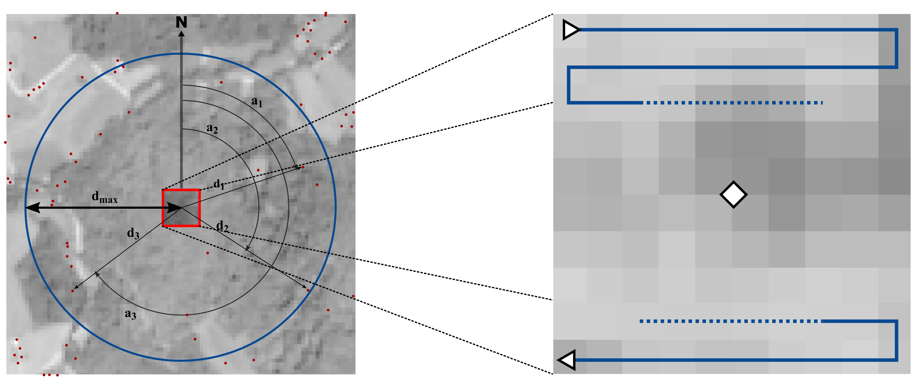
3.2.1. GSCM Construction

In order to train a deep learning model, input data has to be formatted as numerical values in vectors. Therefore, nominal descriptions provided by the semantics are transformed to a new feature space using a GSCM [40], where the records are the samples and the fields are the feature space. Once this matrix is computed, it can be linked to the remotely sensed imagery, extending the GSCM with information on the optical reflectances.
Consider a single grid cell provided by the CORINE LULC dataset. It has a geospatial extent of 100 m × 100 m and a label describing its LULC class. Additional to the grid cell, vector data from LinkedGeoData is present within and outside the grid cell. This vector data contains geo-objects with two attributes, its location (point geometry), and its OWL class. A feature vector for this grid cell is computed, containing descriptive statistics for each OWL class which is present within the grid cell as well as in a defined proximity d m a x around the grid cell centre (see Figure 2, left side): all geo-objects within a distance d m a x to the cell centre are described. Based on this subset of geo-objects, seven descriptive statistics are computed for each OWL class: (1) the minimum distance from the cell centre to a geo-object of this class, (2) the maximum distance to a geo-object of this class from the cell centre, (3) the standard deviation of all distances from the cell centre to geo-objects of this class, (4) the minimum azimuth from the cell centre to a geo-object of this class, (5) the maximum azimuth from the cell centre to a geo-object of this class, (6) the standard deviation of all azimuths from the cell centre to a geo-object of this class, and, (7) the number of geo-objects of this class. As the OWL classes are structured in an ontology, each geo-object can be part of multiple classes. A geo-object of class Pet shop, for example, is also of class Shop. A geo-object is included in all calculations of the descriptive statistical values for each OWL class it is part of. Thus, a geo-object of class Pet shop is not only included in calculating the descriptive values for class Pet shop but all of its parent classes (e.g., Shop and Amenity). The final feature vector contains these seven descriptive values for each class within the proximity of d m a x to the grid cell centre. In cases where there is no geo-object within the proximity d m a x , the corresponding grid cell is excluded from the procedure, as there is no data available around it. In cases where a specific OWL class is not present in the subset of geo-objects which are around the cell centre, its corresponding descriptive values are set by default values of d m a x for descriptive values (1), (2), and 0 for the other descriptive values. A matrix is formed when the procedure for creating a single vector based on semantics is undertaken for multiple grid cells (observations). This is the Geospatial Configuration Matrix (GSCM) [40].
Each row of the GSCM is a sample. It contains the descriptive values as well as the LULC class label which has to be classified correctly. The parameter d m a x defines the maximum distance in which geo-objects and their OWL classes are considered around a grid cell. Thus, d m a x parameterises the first law of Geography [44]. The GSCM can have up to 9100 columns (7 descriptive statistical values for 1300 OWL classes). One critical part of the experiments was to determine an optimal value for d m a x . We used the thresholds suggested by [40]: 20 m, 50 m, 500 m, 1 km, 5 km, 10 km, and 30 km. For every d m a x value a separate GSCM was computed. These were used in Experiments 1 and 2 to assess the impact of different maximum distances used to extract geo-objects.

3.2.2. Linking Semantic and Image Information

The Sentinel-2 image information within a CORINE grid cell was clipped and attached to the corresponding GSCM (see Figure 2, right side). As the dimension of each CORINE grid cell is 100 m × 100 m and the imagery has a resolution of 10 m × 10 m, the clipped image is sized 10 pixel × 10 pixel. These clipped images were then vectorized and the average and standard deviation of each channel were appended to an ordered sequence of then having 1122 elements ((width × height +2) × 11 channels).
Each vector was then appended to the corresponding GSCM row, resulting in a GSCM of 10,222 fields ( 9100 + 1122 ) , composed of 2 sub matrices: one of the semantic information, denoted as S and another containing the image information, denoted as I. This GSCM therefore had the form G S C M = [ S | I ] . In Experiment 1, both sub matrices were used for the classification, thus, G S C M = [ S | I ] . For Experiment 2 only S, the geospatial semantics was used to classify the LULC, with I omitted resulting in G S C M = [ S ] . Experiment 3 used only the image information, thus G S C M = [ I ] . For each LULC class, 12,000 samples were used for training and testing (156,000 samples in total). As seven different d m a x thresholds were used, seven different matrices were evaluated for Experiment 1 and Experiment 2 to assess the impact of each distance on the semantic information incorporated into the analyses. Experiment 3 used one matrix of the image information for all selected grid cells.

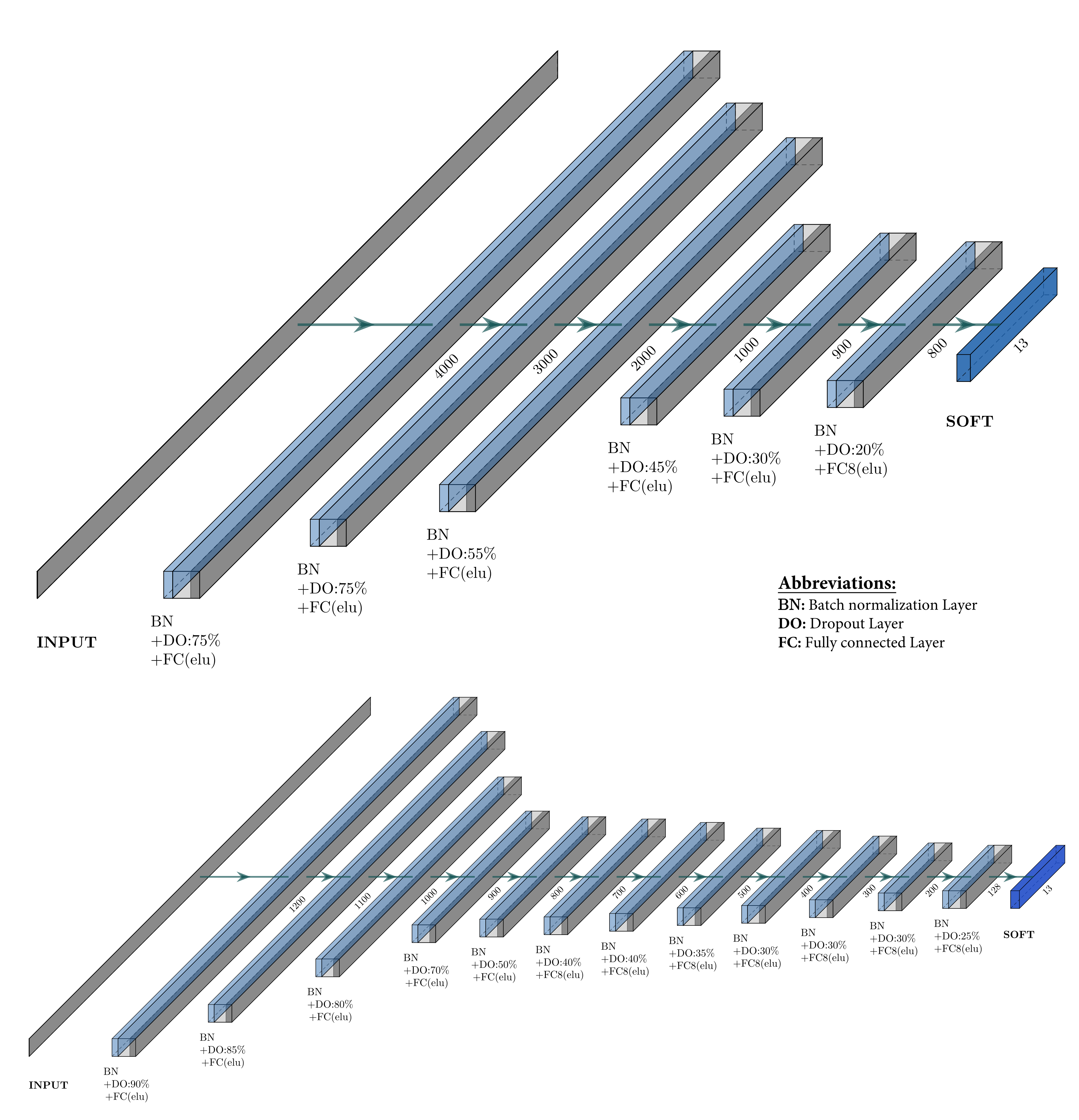
3.2.3. Model Selection and Evaluation

After the GSCMs were constructed, deep learning was performed for LULC classification. However, first, a suitable deep learning model had to be found for each experiment. A multilayer perceptron (MLP) was applied to each experiment, as this was the optimal network type reported by [40]. Next, optimal hyperparameters were determined for the MLP model of each experiment in two steps: (1) finding optimal MLP models for each distance threshold d m a x by combining manual as well as random searches of the hyperparameters. As a result, a MLP architecture was obtained as well as a d m a x value for which the LULC classification worked best in the experiments; (2) given the optimal d m a x value, a second more precise hyperparameter search for the MLP was performed to ensure that the final MLP model was the most suitable, using a nested cross-validation. These steps are explained in detail in the next sections.
Step 1: The activation functions, number of neurons, and the optimiser function were searched for using a combination of manual and random search. Random search was used rather than systematic search, as literature suggests its superiority [45]. The performance of every potential model was internally evaluated through a 10-fold cross-validation to avoid overfitting in the final model. Afterwards, the best model for each experiment was chosen, based on the overall accuracy and the kappa coefficient. For Experiments 1 and 2, this was done for each maximum distance threshold d m a x . As Experiment 3 used remotely sensed imagery only, it did not depend on the threshold d m a x . Therefore, the 10-fold cross-validation was done for each potential model in Experiment 3 but not for multiple d m a x threshold values. After this validation procedure, a d m a x value was obtained which yielded the highest classification accuracy as well as its optimal MLP model for each experiment.
Step 2: A final 5-fold nested cross validation was computed for each experiment, in order to gain confidence that the corresponding MLP models were optimal. In contrast to a normal cross-validation, the nested cross-validation computes an optimal classification model within every fold, by applying a hyperparameter search. We applied a randomised search with an increased hyperparameter search space compared to Step 1. As a nested cross-validation can yield long runtimes due to its computational complexity, we employed it only for the optimal d m a x values for each experiment. Thus, a 5-fold nested cross-validation was undertaken for Experiments 1, 2, and 3, in which three different hyperparameters could be chosen from: (1) the number of layers {1, 2, 3, 4, 5}; (2) the number of neurons a layer has {1400, 1300, 1200, 1100, 1000, 900}, and (3) the dropout rate {0.1, 0.2, 0.3, 0.4, 0.5, 0.6}. In this case, the 5-fold nested cross-validations did not identify classification models with higher overall accuracies or kappa coefficients than were already found. Future research will focus on hyperparameter searching to an even greater degree than undertaken here as the focus of this work is to illustrate the potential of semantics and its fusion with remotely sensed imagery for LULC classification, rather than hyperparameter searching.

3.2.4. Analyses

For each experiment, an accuracy assessment was made using overall accuracy, kappa, producer’s accuracy (recall), and user’s accuracy (precision). This allowed the different experiments to be compared quantitatively. These metrics are defined as follows:
Overall accuracy:
overall accuracy = number of all correct predictions number of all wrong predictions
Kappa [46]:
κ = p 0 p c 1 p c
where p 0 is defined as the proportion of correct predictions and p c as the expected proportion of predictions due to chance [46].
User’s and producer’s accuracy (precision and recall, respectively):
recall = t p t p + f n precision = t p t p + f p
where t p refers to true positive, f p to false positive and f n to false negative.
For the classification model with the highest overall accuracy and kappa coefficient for each experiment, a qualitative assessment was performed. Two major aspects were considered:
(1)
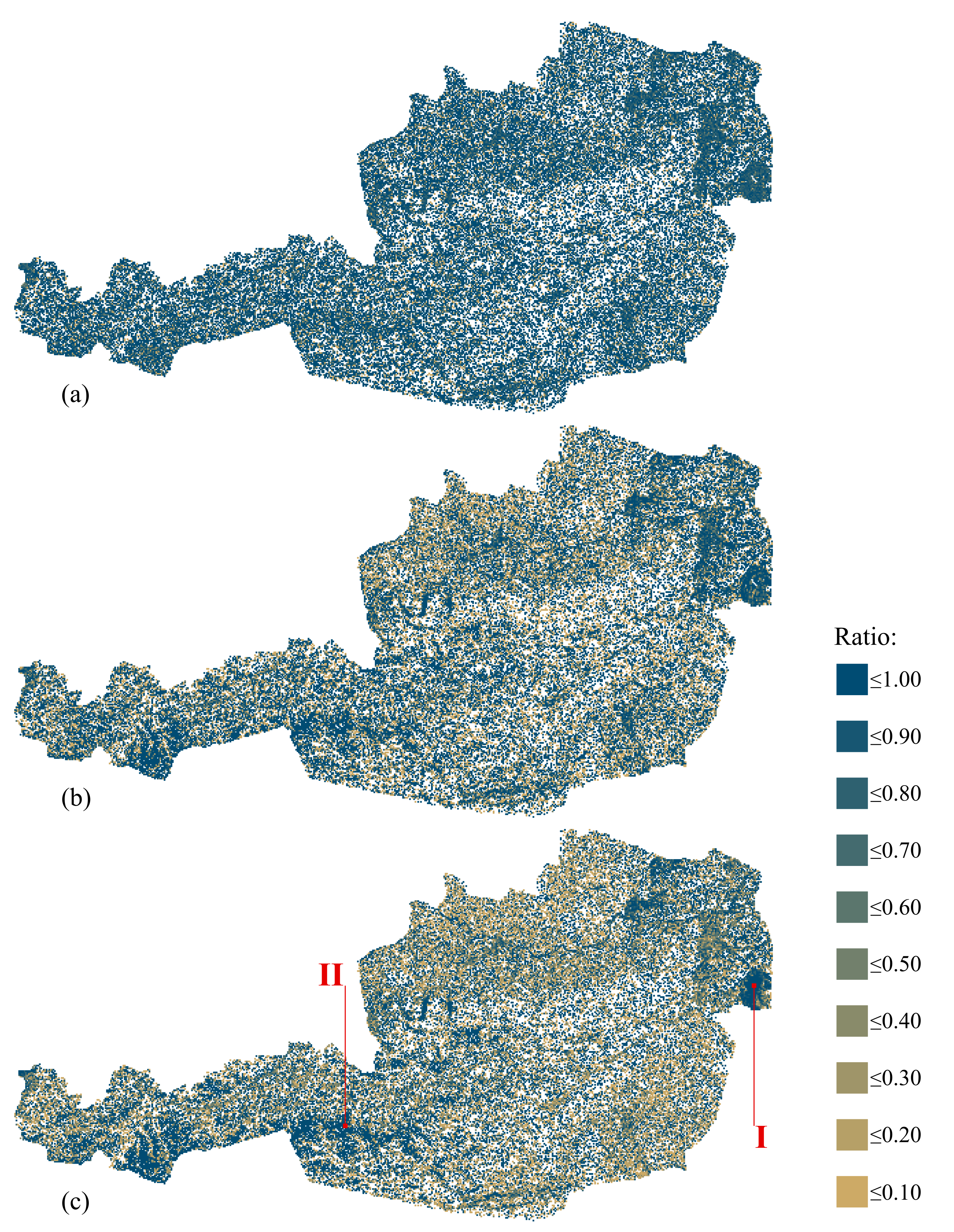
The geographical distribution of the classification error. Here, a grid covering the study area was used and the ratio of correctly versus incorrectly samples was computed for each grid cell. The grid cell size was set by the d m a x value which yielded the highest classification scores;
(2)
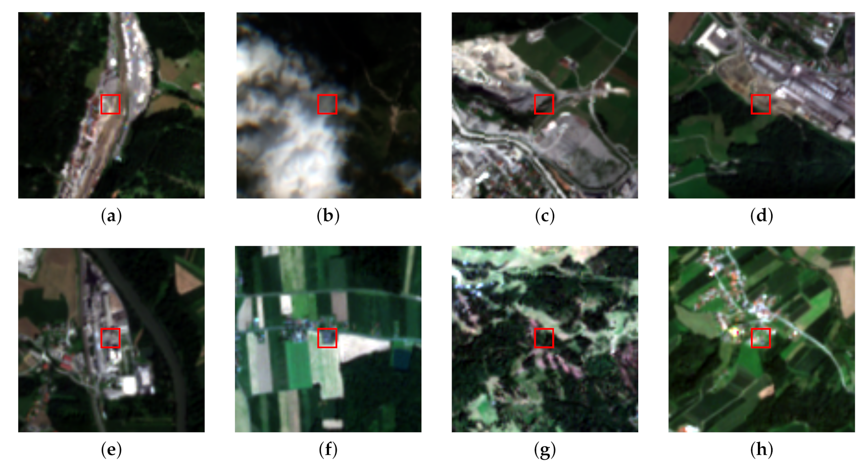
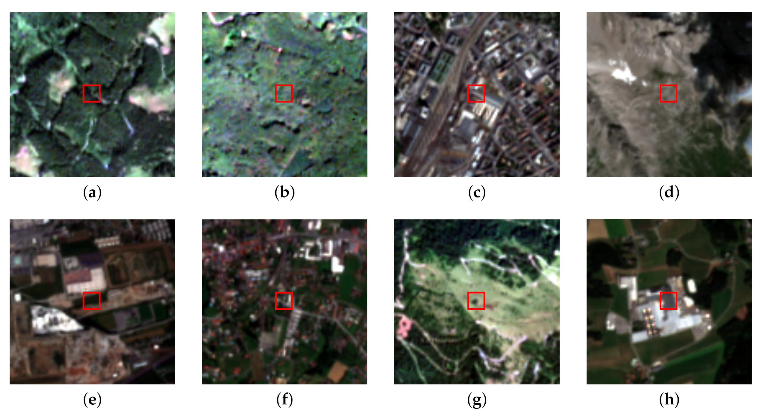
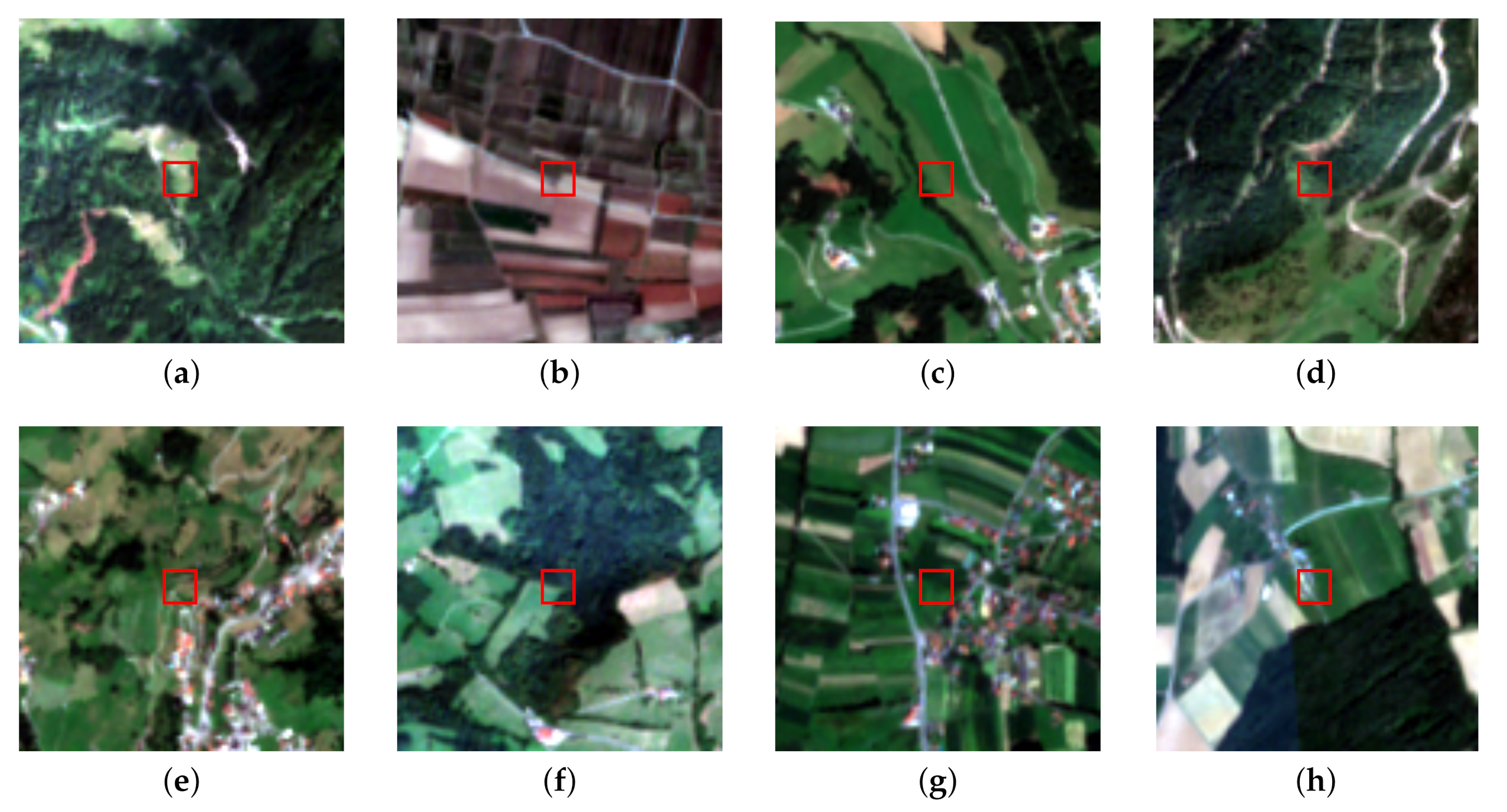
Selected samples and their surrounding were then visually explored. For this purpose, the Sentinel-2 image was extracted around the corresponding grid cells. This enabled insights to be gained on the characteristics of the input data used. For example, some samples were classified correctly with using semantics only but not using imagery only. This might be due to the surrounding geo-objects as well as the imagery. The aim here was to examine classified samples and to determine potential characteristics in common. Four types of samples were defined: (1) samples correctly classified in Experiment 2 (semantics only) but not in Experiment 3 (imagery only) to examine the potential advantages of using semantics only over using imagery only. (2) samples classified correctly in Experiment 3 but not in Experiment 2. These samples illustrate cases where the imagery only approach provides higher classification accuracy than using semantics only. (3) samples which were correctly classified in both Experiment 2 and Experiment 3. (4) samples classified correctly in Experiment 1 but not in Experiments 2 and 3. These samples highlight situations when semantics as well as imagery only were not sufficient alone to classify correctly but were once fused.
The potential of using geospatial semantics for LULC classification as well as its synergies with remotely sensed imagery for this purpose were identified through these quantitative and qualitative assessments.

4. Results and Analysis

The accuracy assessments of the three experiments are summarised in Table 2. Using the data fusion, the highest accuracies were generated (OA of 82.18% and a kappa coefficient of 0.8069). A d m a x of 1 km provided the highest accuracies for Experiment 1 and 2. The MLP model architectures can be seen in Figure 3. Experiments 1 and 2 had the same optimal MLP model architecture. The corresponding hyperparameters can be seen in Table 3.
Between using semantics only and imagery only, semantics only provided a more accurate classification, with an overall accuracy of 76.11 % and a kappa coefficient of 0.7412. Using remotely sensed imagery only, an overall accuracy of 65.52 % and a kappa coefficient of 0.6264 was scored. Observing the effect of the d m a x threshold in Table 2, it can be seen that the accuracies first increase (indicated by both overall accuracy and kappa coefficient); however, they decrease once d m a x increases above 1 km, for Experiments 1 and 2.
Table 4 and Table 5 show producer’s and user’s accuracy. They show that increasing d m a x increases the classification accuracy for single LULC classes. In addition, it can be observed that the user’s accuracy is more homogenously distributed than the producer’s accuracy, for Experiment 1 and 2. However, there is one exception, namely LULC class I, i.e., urban fabric. Using semantics only, Experiment 2 (see Table 5), it can be seen that producer’s accuracy is the highest when d m a x is set to 20 meters and decreases with an increasing d m a x value. This stands in contrast to the user’s accuracy of urban fabric for this experiment which increases with increasing d m a x . Observing the remaining LULC classes in Table 4 and Table 5 for Experiment 1 and 2 it can be seen that LULC IX (Forest) has the lowest producer’s accuracies for most d m a x thresholds using semantics only. This changes too, when the classification is based on fused semantics and imagery, and, in Forest, the majority of its producer’s accuracy values are not the lowest. In Experiment 3 (see Table 5, right side) LULC classes which have a higher producer’s as well as user’s accuracy seem to benefit the most from the data fusion.
The confusion matrices can be seen in Figure 4 and Figure 5. They reveal that single data source generates higher classification accuracies for specific LULC classes, while the data fusion seems to combine these benefits. In particular, for Experiment 2 (Figure 4b), i.e., using semantics only, over 90% of the samples of LULC classes II, III, IV, VI, and XII were classified correctly. They correspond to Industrial, commercial, and transport units, Mine, dump, and construction sites, Artificial, non-agricultural vegetated areas, Permanent crops, and Inland wetlands, respectively. Only LULC Forest is below 50% accuracy for Experiment 2, which was mostly confused with Arable land, Pastures, and Scrub and/or herbaceous vegetation associations. Urban fabric (LULC class I) was classified with an accuracy of 58% and was mostly confused with Pastures for Experiment 2. These values changed once the data fusion was used (Experiment 1, see Figure 4a), where LULC class Urban fabric was classified with an accuracy of 71%.
The confusion matrix for Experiment 3, which was based on imagery only, can be seen in Figure 5. Here, the highest classification accuracy was obtained for class Inland waters and classes Open spaces with little or no vegetation as well as Permanent crops. In this experiment, the highest confusions can be observed for Scrub and/or herbaceous vegetation associations and Artificial, non-agricultural vegetated areas, Heterogeneous agricultural areas and Arable land, and Pastures and Heterogeneous agricultural areas.
The geographical distribution of classification errors can be seen in Figure 6. Subfigures a–c show the geographical distributions of the classification accuracy of Experiment 1, Experiment 2, and Experiment 3, respectively.
Figure 6a–c show colored 1 km × 1 km grids cells over Austria, each illustrating the ratio of the overall accuracies. A ratio of 1 states that 100% of the samples within a grid cell were classified correctly, whereas 0.60 suggest that 60% of the samples within a grid cell were classified correctly. Grid cells with the highest ratio are colored dark blue and as the ratio decreases, it shifts to beige. A grid size of 1 km × 1 km was chosen for the visualisation here, as this corresponds to the optimal d m a x value we computed. Observing Figure 6, several differences in the geographical distributions of the classification errors can be observed. For Experiment 1, most grid cells are coloured dark blue and distributed homogeneously over the ROI, illustrating that most of the samples were classified correctly. Overall, in subfigure b, fewer grid cells are coloured dark blue than in subfigure a but more than in subfigure c, matching the observations of the accuracy assessment. Considering the geographical distributions of dark blue grid cells, Figure 6b,c exhibit differences: subfigure c shows clusters of dark blue grid cells, one in the east of Austria at a lake (location I). This confirms the high classification accuracy for inland waters using imagery only.
The second cluster lays within the Alps (location II), confirming the high classification accuracy for LULC class Open spaces with little or no vegetation (such as mountains) when using imagery only. In contrast, Figure 6b does not seem to exhibit such strong clusters. A series of areas are beige in both Figure 6b,c; however, the corresponding areas in subfigure a are dark blue. This indicates that both data sources complement each other efficiently once fused.
Figure 7, Figure 8, Figure 9 and Figure 10 show examples of correct and incorrect classifications. In each picture, the Sentinel-2 imagery and a red square, indicating the 100 m × 100 m CORINE LULC grid cell, are shown. Each picture extend is 1 km × 1 km, corresponding to d m a x under which the most accurate classifications were found. Figure 7a–h depict examples of cases where classifications based on semantics only (Experiment 2) were correct but classifications based on imagery only (Experiment 3) only were incorrect. Figure 8a–h illustrate cases where the classification based on imagery alone was correct, but where the classification based on semantics failed to classify correctly. Figure 9a–h show cases where both classifications worked correctly. Additionally, Figure 10a–h show examples of cases in which the classification using the fusion of both semantics and imagery worked (Experiment 1) but using semantics and imagery alone (Experiments 2 and 3) failed. Please note that the 32 examples were manually selected from a random selection of the 1200 samples in each class. The 32 samples were selected to be representative and to highlight the advantages and disadvantages of each classification approach.
Considering Figure 7, a series of insights can be obtained. Although the Sentinel-2 imagery used was subject to cloud removal, some clouds remained (Figure 7b). Its LULC class is Artificial, non-agricultural vegetated areas which was classified correctly when using semantics only but classified wrongly when using imagery only. Another aspect which can be seen in the remaining images of Figure 7 is that the LULC to be classified are related to man-made structures. For example, Figure 7 might appear as a forest at first glance; however, it is part of a ski slope in the mountains, making it a LULC of Artificial, non-agricultural vegetated areas. The remaining six subfigures show areas with man-made structures, such as Industrial, commercial, and transport units, Mine, dump, and sites, Urban fabric, or Permanent crops.
This behaviour changes in scenes of Figure 8. This shows cases where when using imagery only, the classification worked correctly but when using semantics only, the classification failed. Some grid cells (red squares) here are associated with LULC classes of natural green spaces but have a few man-made structures within their proximity (Figure 8b,c,e,g). For example, in Figure 8b, the grid cell to be classified is within a forest; however, it is surrounded by man-made structures such as streets and houses. Other grid cells are within a 1 km × 1 km area, which contains a mixture of different man-made structures (Figure 8d,f,h). Finally, Figure 8a shows a grid cell which is in a homogenous industrial area with a river in its proximity. In this case, the classification using semantics only yielded Inland waters whereas the classification using imagery only predicted correctly that the grid cell is an instance of the LULC class Industrial, commercial, and transport units. The discriminative power of using semantics only seems to suffer from such mixed cases.
In Figure 9a–h, eight scenes are shown in which both approaches, using semantics only and imagery only, yield correct classification results. Here, most images show a homogenous surface (see Figure 9a–e). For example, Figure 9b shows forest only and Figure 9d shows mountainous area only. Furthermore, Figure 9g,h show scenes in which the imagery is consistent within the red square and its immediate surrounding and the semantic sources are evenly spread around the red square. In Figure 9g forest is present in almost every direction around the red square while in Figure 9h, an industrial compound is present within as well as around the red square.
Figure 10a–h show cases where the fusion of semantics and imagery (Experiment 1) classified correctly, but classifications based on semantics only and imagery only yielded incorrect results. In Figure 10a–h, two aspects can be observed: (1) within the red squares the imagery is mixed. For example, in Figure 10a,c,d,f,g, the imagery within the red square is mixed with forest-like texture as well as grassland-like texture. (2) Figure 10c–g contain no semantic information (building, streets, etc.) within the red square but only outside of it.

5. Discussion

There are two major findings from this work. First, LULC can be classified using semantics only. In our experiments we found that the semantics of geo-objects provide meaningful information and enable the corresponding LULC class to be determined. Second, fusing semantics with imagery enhanced the classification results. Their combination complemented and increased the accuracy of the LULC classification, compared to using the two single data sources alone. Additionally, some LULC classes were predicted better than others using semantics only instead of using imagery only, which is reflected in the accuracy assessments and the qualitative analyses. This performance is discussed below from two perpectives: the first examines the overall performance of the LULC classifications and the second discusses the per class accuracies. The qualitative analysis are also discussed and highlight how semantics can be used as an information source in LULC classification.

5.1. Overall Classification Results

The overall accuracies as well as kappa coefficients suggest not only that LULC can be classified based on semantics but also that the fusion with imagery yields improved results. The impact of d m a x is important, and it was found to have an optimal value in Experiments 1 and 2, decreasing accuracy if it was higher or lower than this value. A potential explanation for this is that d m a x controls the area from which OWL class information is obtained from geo-objects around a sample. Thus, a low d m a x value results in too little local information about the types of nearby geo-objects. In contrast, a higher d m a x value results in the loss of valuable local information, as the computation of the feature vector relies on aggregation functions, such as the standard deviation and the maximum. However, despite the impact of d m a x , the fusion of imagery and semantics was always found to be superior to the classification using semantics only, for any d m a x value. This suggests that semantics, when used as auxiliary information to imagery, complement it in a meaningful way, independent of the d m a x value.

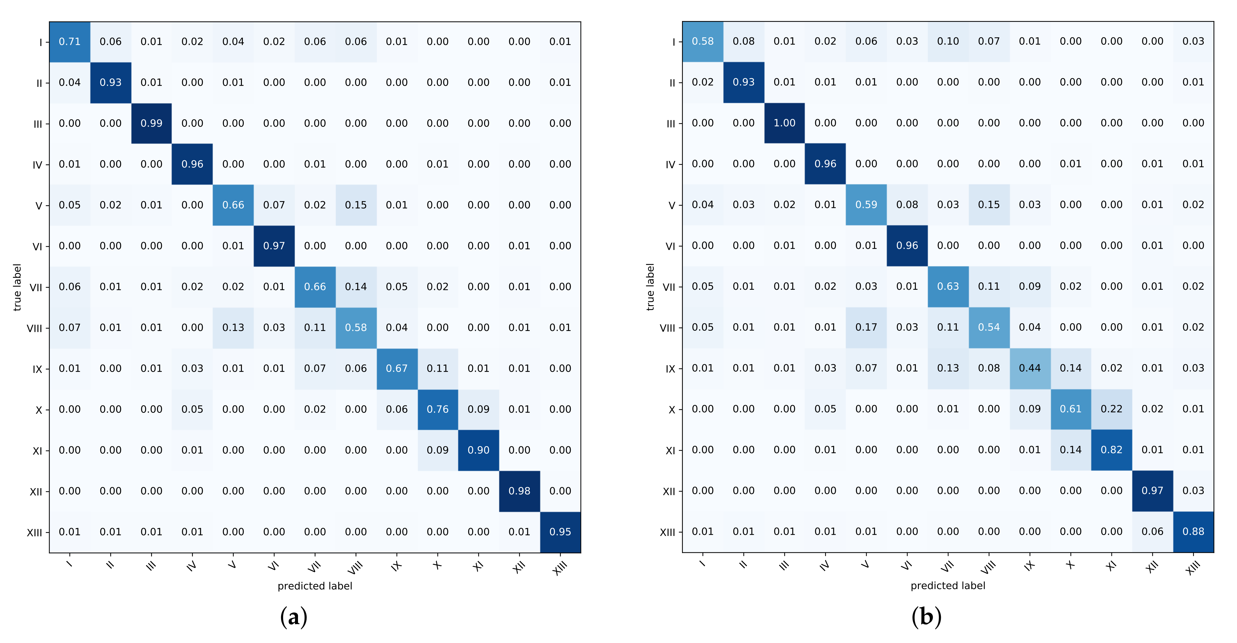
5.2. Classifications of Single Classes

The results showed that geospatial semantics predict certain LULC classes better than others and that the fusion of both semantics and remotely sensed imagery created a synergy, which yielded superior per class accuracies. For example, LULC class I (Urban fabric) was classified with a similar accuracy from single data sources (see Figure 4b and Figure 5), but the fusion resulted in a superior classification accuracy (see Figure 4a). The same was true for class V (Arable land), VIII (Heterogeneous agricultural areas), X (Scrub and/or herbaceous vegetation associations), XI (Open spaces with little or no vegetation), XII (Inland wetlands), and XIII (Inland waters). The biggest classification improvements using the fused data were found for LULC classes Urban fabric. A potential explanation for this is that semantics complement the imagery well for this class. The semantics allow areas with a similar spectral signature but different underlying LULC class to be differentiated and vice versa. In general, the LULC classes were classified more accurately when the data fusion were used, overcoming the confusion within and between LULC classes when semantics only and imagery only were used. For example, while Urban fabric was mostly confused with class II (Industrial, commercial, and transport units) using imagery only, it was mostly confused with class VII (Pastures) using semantics only. Consequently, using the fused, the classification model is able to better distinguish between Urban fabric and Industrial, commercial, and transport units when semantics are included and can differentiate better between Urban fabric and (Pastures) using information from imagery. For LULC classes Industrial, commercial, and transport units (class II), Mine, dump, and construction sites (class III), Artificial, non-agricultural vegetated areas (class IV), and, Inland wetlands (class XII), semantics only was sufficient to achieve classification accuracies of over 90%. In order to provide a potential explanation for this, it has to be remembered that the used semantics is based on LinkedGeoData, which itself is based on OSM data. Thus, some regions might have greater coverage (and thus more mapped objects), providing more semantics. As such, classes II–IV could potentially benefit from this fact, as they are related to man-made structures, increasing the likelihood that relevant local data is captured by OSM volunteers. Furthermore, specific OWL classes could improve the detection of these LULC classes. For example, residential houses and an industrial complex might look similar on satellite imagery, while OWL classes can describe them with meaningful concepts such as residential house and factory, allowing a distinction of areas based on their functions and usage. In contrast to that, two LULC classes were classified more accurately with imagery only, than with semantics only, namely, classes V (Arable land) and IX (Forest). A potential reason for semantics to score a lower classification accuracy for these two classes could be that OWL classes from LinkedGeoData exhibit less significant associations to non-urban areas than to urban areas [42]. Thus, semantics in these areas might be too sparse to improve the classification.

5.3. Semantics for LULC Classification

Geospatial semantics exhibit different characteristics to conventional sensor data like optical imagery, when classifying LULC. For example, semantics rely on nominal values while optical imagery relies on ratios obtained from electromagnetic reflectance. As such, geospatial semantics reflect the meaning of geo-objects, such as Building or Bench and not their physical characteristics. In the case of LinkedGeoData, this is derived from OSM, which is created by volunteers. They capture and annotate the vector data, making themselves the sensors. This consequently enables the inclusion of a variety of different geo-object meanings into the LULC classification, as captured by the crowd of volunteers. As such they provide potentially specific and meaningful class descriptions. For example, OWL class Peak is typically recorded on mountains and can therefore help to find the corresponding LULC class Open spaces with little or no vegetation (see Figure 9d). Another example for such a characteristic OWL class is Chair-lift which often occurs close to skiing areas/slopes. Here, the OWL class can help to identify slopes which are of LULC class Artificial, non-agricultural vegetated areas (see Figure 7). However, the advantage of having specific and meaningful OWL classes can become a disadvantage too: an industrial area can have OWL class River in the proximity, rendering the final LULC classification to Inland waters instead of Industrial, commercial, and transport units (see Figure 8a). In general, an even geographic distribution of characteristic geo-objects within the proximity of d m a x was found to foster a correct LULC classification when using semantics only. For example, Figure 9c,e,f, show such situations. Here, the entire 1 km × 1 km scene is covered with geo-objects. By contrast, in some cases, geo-objects are present within the proximity of d m a x , but the sample grid cell belongs to a LULC atypical for them. An example of such cases can be seen in Figure 8c,g: here, geo-objects such as houses might have led the classifier to compute that the samples are of LULC class Urban fabric, although they are of LULC class Pastures and Forest, respectively. This is likely to be due to the information around these grid cells (the red squares) being dissimilar to their surroundings. If the grid cell of the LULC is similar to geo-objects within the d m a x proximity, the classifications tend to be often correct. Examples for such cases can be seen in Figure 7a,c–e,h as well as Figure 9h. However, an important aspect of semantics as a data source becomes apparent when looking at Figure 7: any image effects such as clouds do not affect the semantics. In general, geospatial semantics rely on observations made by volunteers on the ground which, unlike spaceborne or airborne observations, do not need atmospheric corrections.

5.4. Future Work

This work makes a first step towards a new research domain which aims at understanding the relationship between semantics and LULC classification. It has deepened our understanding of the potential use of semantics for this task. This could be extended further by examining the impact of the ontology, which is the structure of OWL classes, as in the LinkedGeodata. However, perhaps an ontology with a deeper or wider structure, providing more specific or more classes overall, respectively, could improve the accuracy even further. Thus, this research direction would focus on the ontology as a classification parameter. Semantics allow space to be described in terms of meaning, which could be used for novel analysis methods, through, for example, the use of explainable artificial intelligence (XAI) to determine which types of geo-objects (OWL classes) are relevant for specific LULC classes. This would enable one to relate LULC classes to meaningful and human understandable concepts (OWL classes) and therefore help one to understand LULC in a novel way. Next to the investigation of the role of geospatial semantics for LULC classification, advanced deep learning architectures could be explored in future research in order to improve the classification accuracy even further. Particularly, networks with residual connections, convolutional neural networks [47] (for the images—as a separate input branch of the ANN), or attention mechanisms [48] could be employed to score even higher classification accuracies. Furthermore, other types of machine learning algorithms, such as support vector machines, could be explored too. Here, semantics were fused with a single image (mosaic) in feature space; future work can research how to combine semantics with multi-temporal imagery in an effective manner. Additionally, other types of remotely sensed imagery could be used, such as hyperspectral [49] or synthetic aperture radar [50] imagery. CORINE is associated with a certain classification accuracy itself, as such, our results come with the corresponding caveat as we rely on it as being the ground truth. Other sources on LULC ground truth could therefore be used in future work. Furthermore, not only a single source for ground truth could be used but a combination of different sources, increasing the overall reliability. In this work geospatial semantics were obtained from LinkedGeoData (http://linkedgeodata.org/ accessed on 5 January 2021) for the region of Austria. Data outside of Austria can be obtained from them as well, being the base for future work, which studies how Semantic Boosting works in other ROIs. Additionally, we plan on releasing the processed GSCM data for Austria as well as outside of Austria (for future studies).

6. Conclusions

The focus of this research was to investigate the inclusion of geospatial semantics within a LULC classification of remotely sensed imagery. For this purpose a GSCM was used and extended in order to combine the image information and semantics at a feature level. The results show that when geospatial semantics are fused with remotely sensed imagery, LULC classification accuracies are increased. In particular, LULC classes which relate to man-made structures, such as Urban fabric, are classified with higher accuracy, once the combination is used. Furthermore, geospatial semantics alone were shown to support the classification of LULC classes with promising accuracy, especially for LULC classes, which relate to specific land use, such as mines or industrial areas. The qualitative analysis showed, that in a series of cases, semantics enabled one to classify areas correctly, which would have otherwise been confused with other LULC classes, which have similar spectral signatures (e.g., Artificial, non-agricultural vegetated areas and Scrub and/or herbaceous vegetation associations). Next to the accuracy assessment and the qualitative analysis, the geographical distribution of the classification accuracy was analysed. Here, it was found that the combination of both information sources (imagery and semantics) yield correct LULC classifications, which are homogeneously spread in the study area, while the single sources yield LULC classifications which are more clustered in some regions. Overall, the results show that geospatial semantics are a fruitful source for LULC classification, especially once it is combined with imagery.

Author Contributions

Conceptualization, M.M.C.; methodology, M.M.C., I.G.; software, M.M.C., M.C.; validation, M.M.C., I.G., A.J.C.; formal analysis, M.M.C., I.G. and A.J.C.; investigation, M.M., I.G. and A.J.C.; resources, M.M.C. and I.G.; data curation, M.M.C.; writing—original draft preparation M.M.C., I.G. and A.J.C.; writing—review and editing, M.M.C., I.G. and A.J.C.; visualization, M.M.C.; supervision, I.G.; project administration, M.M.C. All authors have read and agreed to the published version of the manuscript.

Funding

This research received no external funding.

Data Availability Statement

The data presented in this study are available on request from the corresponding author.

Conflicts of Interest

The authors declare no conflict of interest.

References

  1. Comber, A.; Fisher, P.; Wadsworth, R. What is Land Cover? Environ. Plan. B Plan. Des. 2005, 32, 199–209. [Google Scholar] [CrossRef] [Green Version]
  2. Fisher, P. The pixel: A snare and a delusion. Int. J. Remote Sens. 1997, 18, 679–685. [Google Scholar] [CrossRef]
  3. Foody, G.M. Harshness in image classification accuracy assessment. Int. J. Remote Sens. 2008, 29, 3137–3158. [Google Scholar] [CrossRef] [Green Version]
  4. Foley, J.A. Global Consequences of Land Use. Science 2005, 309, 570–574. [Google Scholar] [CrossRef] [Green Version]
  5. Pielke, R.A. Land Use and Climate Change. Science 2005, 310, 1625–1626. [Google Scholar] [CrossRef] [PubMed] [Green Version]
  6. Turner, B.L.; Lambin, E.F.; Reenberg, A. The emergence of land change science for global environmental change and sustainability. Proc. Natl. Acad. Sci. USA 2007, 104, 20666–20671. [Google Scholar] [CrossRef] [Green Version]
  7. Polasky, S.; Nelson, E.; Pennington, D.; Johnson, K.A. The Impact of Land-Use Change on Ecosystem Services, Biodiversity and Returns to Landowners: A Case Study in the State of Minnesota. Environ. Resour. Econ. 2011, 48, 219–242. [Google Scholar] [CrossRef]
  8. De Chazal, J.; Rounsevell, M.D. Land-use and climate change within assessments of biodiversity change: A review. Glob. Environ. Chang. 2009, 19, 306–315. [Google Scholar] [CrossRef]
  9. Kuhn, W. Geospatial Semantics: Why, of What, and How. In Journal on Data Semantics III; Spaccapietra, S., Zimányi, E., Eds.; Springer Berlin Heidelberg: Berlin/Heidelberg, Germany, 2005; pp. 1–24. [Google Scholar]
  10. Bengana, N.; Heikkilä, J. Improving Land Cover Segmentation Across Satellites Using Domain Adaptation. IEEE J. Sel. Top. Appl. Earth Obs. Remote Sens. 2021, 14, 1399–1410. [Google Scholar] [CrossRef]
  11. Antropov, O.; Rauste, Y.; Šćepanović, S.; Ignatenko, V.; Lönnqvist, A.; Praks, J. Classification of Wide-Area SAR Mosaics: Deep Learning Approach for Corine Based Mapping of Finland Using Multitemporal Sentinel-1 Data. In Proceedings of the IGARSS 2020 IEEE International Geoscience and Remote Sensing Symposium, Ahmedabad, Gujarat, India, 2–4 December 2020; pp. 4283–4286. [Google Scholar] [CrossRef]
  12. Balado, J.; Arias, P.; no, L.D.V.; González-deSantos, L.M. Automatic CORINE land cover classification from airborne LIDAR data. Procedia Comput. Sci. 2018, 126, 186–194. [Google Scholar] [CrossRef]
  13. Balzter, H.; Cole, B.; Thiel, C.; Schmullius, C. Mapping CORINE Land Cover from Sentinel-1A SAR and SRTM Digital Elevation Model Data using Random Forests. Remote Sens. 2015, 7, 14876–14898. [Google Scholar] [CrossRef] [Green Version]
  14. Stadler, C.; Lehmann, J.; Höffner, K.; Auer, S. LinkedGeoData: A Core for a Web of Spatial Open Data. Semant. Web J. 2012, 3, 333–354. [Google Scholar] [CrossRef]
  15. Pielke, R.A., Sr.; Pitman, A.; Niyogi, D.; Mahmood, R.; McAlpine, C.; Hossain, F.; Goldewijk, K.K.; Nair, U.; Betts, R.; Fall, S.; et al. Land use/land cover changes and climate: Modeling analysis and observational evidence. WIREs Clim. Chang. 2011, 2, 828–850. [Google Scholar] [CrossRef]
  16. Tayebi, M.; Fim Rosas, J.T.; Mendes, W.D.S.; Poppiel, R.R.; Ostovari, Y.; Ruiz, L.F.C.; dos Santos, N.V.; Cerri, C.E.P.; Silva, S.H.G.; Curi, N.; et al. Drivers of Organic Carbon Stocks in Different LULC History and along Soil Depth for a 30 Years Image Time Series. Remote Sens. 2021, 13, 2223. [Google Scholar] [CrossRef]
  17. Li, Z.; White, J.C.; Wulder, M.A.; Hermosilla, T.; Davidson, A.M.; Comber, A.J. Land cover harmonization using Latent Dirichlet Allocation. Int. J. Geogr. Inf. Sci. 2020, 35, 1–27. [Google Scholar] [CrossRef]
  18. Craglia, M.; de Bie, K.; Jackson, D.; Pesaresi, M.; Remetey-Fülöpp, G.; Wang, C.; Annoni, A.; Bian, L.; Campbell, F.; Ehlers, M.; et al. Digital Earth 2020: Towards the vision for the next decade. Int. J. Digit. Earth 2012, 5, 4–21. [Google Scholar] [CrossRef]
  19. Goodchild, M.F.; Guo, H.; Annoni, A.; Bian, L.; de Bie, K.; Campbell, F.; Craglia, M.; Ehlers, M.; van Genderen, J.; Jackson, D.; et al. Next-generation Digital Earth. Proc. Natl. Acad. Sci. USA 2012, 109, 11088–11094. [Google Scholar] [CrossRef] [PubMed] [Green Version]
  20. Goodchild, M. The use cases of digital earth. Int. J. Digit. Earth 2008, 1, 31–42. [Google Scholar] [CrossRef]
  21. Metzger, M.; Rounsevell, M.; Acosta-Michlik, L.; Leemans, R.; Schröter, D. The vulnerability of ecosystem services to land use change. Agric. Ecosyst. Environ. 2006, 114, 69–85. [Google Scholar] [CrossRef]
  22. Ma, J.; Heppenstall, A.; Harland, K.; Mitchell, G. Synthesising carbon emission for mega-cities: A static spatial microsimulation of transport CO2 from urban travel in Beijing. Comput. Environ. Urban Syst. 2014, 45, 78–88. [Google Scholar] [CrossRef]
  23. Fu, P.; Weng, Q. A time series analysis of urbanization induced land use and land cover change and its impact on land surface temperature with Landsat imagery. Remote Sens. Environ. 2016, 175, 205–214. [Google Scholar] [CrossRef]
  24. Debbage, N.; Shepherd, J.M. The urban heat island effect and city contiguity. Comput. Environ. Urban Syst. 2015, 54, 181–194. [Google Scholar] [CrossRef]
  25. Fuller, R.; Smith, G.; Devereux, B. The characterisation and measurement of land cover change through remote sensing: Problems in operational applications? Int. J. Appl. Earth Obs. Geoinf. 2003, 4, 243–253. [Google Scholar] [CrossRef]
  26. Hussain, M.; Chen, D.; Cheng, A.; Wei, H.; Stanley, D. Change detection from remotely sensed images: From pixel-based to object-based approaches. ISPRS J. Photogramm. Remote Sens. 2013, 80, 91–106. [Google Scholar] [CrossRef]
  27. Tewkesbury, A.P.; Comber, A.J.; Tate, N.J.; Lamb, A.; Fisher, P.F. A critical synthesis of remotely sensed optical image change detection techniques. Remote Sens. Environ. 2015, 160, 1–14. [Google Scholar] [CrossRef] [Green Version]
  28. Grekousis, G.; Mountrakis, G.; Kavouras, M. An overview of 21 global and 43 regional land-cover mapping products. Int. J. Remote Sens. 2015, 36, 5309–5335. [Google Scholar] [CrossRef]
  29. Thanh Noi, P.; Kappas, M. Comparison of Random Forest, k-Nearest Neighbor, and Support Vector Machine Classifiers for Land Cover Classification Using Sentinel-2 Imagery. Sensors 2017, 18, 18. [Google Scholar] [CrossRef] [Green Version]
  30. Comber, A.; Fisher, P.; Wadsworth, R. Integrating land-cover data with different ontologies: Identifying change from inconsistency. Int. J. Geogr. Inf. Sci. 2004, 18, 691–708. [Google Scholar] [CrossRef] [Green Version]
  31. Mishra, V.N.; Prasad, R.; Kumar, P.; Gupta, D.K.; Dikshit, P.K.S.; Dwivedi, S.B.; Ohri, A. Evaluating the effects of spatial resolution on land use and land cover classification accuracy. In Proceedings of the 2015 International Conference on Microwave, Optical and Communication Engineering (ICMOCE), Odisha, India, 18–20 December 2015; pp. 208–211. [Google Scholar]
  32. Ma, L.; Li, M.; Ma, X.; Cheng, L.; Du, P.; Liu, Y. A review of supervised object-based land-cover image classification. ISPRS J. Photogramm. Remote Sens. 2017, 130, 277–293. [Google Scholar] [CrossRef]
  33. Comber, A.J.; Wadsworth, R.A.; Fisher, P.F. Using semantics to clarify the conceptual confusion between land cover and land use: The example of ’forest’. J. Land Use Sci. 2008, 3, 185–198. [Google Scholar] [CrossRef] [Green Version]
  34. Winter, S. Unified Behavior of Vector and Raster Representation; GeoInfo/GeoInfo, Inst. for Geoinformation, Ed.; University of Technology Vienna: Vienna, Austria, 2000. [Google Scholar]
  35. Comber, A.; Fisher, P.; Wadsworth, R. You know what land cover is but does anyone else?… An investigation into semantic and ontological confusion. Int. J. Remote Sens. 2005, 26, 223–228. [Google Scholar] [CrossRef] [Green Version]
  36. Ríos, S.A.; Muñoz, R. Land Use detection with cell phone data using topic models: Case Santiago, Chile. Comput. Environ. Urban Syst. 2017, 61, 39–48. [Google Scholar] [CrossRef]
  37. Jeawak, S.S.; Jones, C.B.; Schockaert, S. Predicting the environment from social media: A collective classification approach. Comput. Environ. Urban Syst. 2020, 82, 101487. [Google Scholar] [CrossRef]
  38. Schultz, M.; Voss, J.; Auer, M.; Carter, S.; Zipf, A. Open land cover from OpenStreetMap and remote sensing. Int. J. Appl. Earth Obs. Geoinf. 2017, 63, 206–213. [Google Scholar] [CrossRef]
  39. Arsanjani, J.J.; Helbich, M.; Bakillah, M.; Hagenauer, J.; Zipf, A. Toward mapping land-use patterns from volunteered geographic information. Int. J. Geogr. Inf. Sci. 2013, 27, 2264–2278. [Google Scholar] [CrossRef]
  40. Mc Cutchan, M.; Özdal Oktay, S.; Giannopoulos, I. Semantic-based urban growth prediction. Trans. GIS 2020, 24, 1482–1503. [Google Scholar] [CrossRef]
  41. Zhang, Y.; Li, Q.; Tu, W.; Mai, K.; Yao, Y.; Chen, Y. Functional urban land use recognition integrating multi-source geospatial data and cross-correlations. Comput. Environ. Urban Syst. 2019, 78, 101374. [Google Scholar] [CrossRef]
  42. Mc Cutchan, M.; Giannopoulos, I. Geospatial Semantics for Spatial Prediction. In Leibniz International Proceedings in Informatics (LIPIcs), Proceedings of the 10th International Conference on Geographic Information Science (GIScience 2018), Melbourne, Australia, 28–31 August 2018; Winter, S., Griffin, A., Sester, M., Eds.; Schloss Dagstuhl–Leibniz-Zentrum fuer Informatik: Dagstuhl, Germany, 2018; Volume 114, pp. 451–456. [Google Scholar] [CrossRef]
  43. DuCharme, B. Learning SPARQL; O’Reilly Media, Inc.: Sebastopol, CA, USA, 2011. [Google Scholar]
  44. Tobler, W.R. A Computer Movie Simulating Urban Growth in the Detroit Region. Econ. Geogr. 1970, 46, 234–240. [Google Scholar] [CrossRef]
  45. Bergstra, J.; Bengio, Y. Random Search for Hyper-Parameter Optimization. J. Mach. Learn. Res. 2012, 13, 281–305. [Google Scholar]
  46. Cohen, J. A Coefficient of Agreement for Nominal Scales. Educ. Psychol. Meas. 1960, 20, 37–46. [Google Scholar] [CrossRef]
  47. Albawi, S.; Mohammed, T.A.; Al-Zawi, S. Understanding of a convolutional neural network. In Proceedings of the 2017 International Conference on Engineering and Technology (ICET), Antalya, Turkey, 21–23 August 2017; IEEE: New York, NY, USA, 2017; pp. 1–6. [Google Scholar]
  48. Vaswani, A.; Shazeer, N.; Parmar, N.; Uszkoreit, J.; Jones, L.; Kaiser, Ł.; Polosukhin, I. Attention is all you need. In Advances in Neural Information Processing Systems; Curran Associates Inc.: Red Hook, NY, USA, 2017; pp. 5998–6008. [Google Scholar]
  49. Vali, A.; Comai, S.; Matteucci, M. Deep Learning for Land Use and Land Cover Classification Based on Hyperspectral and Multispectral Earth Observation Data: A Review. Remote Sens. 2020, 12, 2495. [Google Scholar] [CrossRef]
  50. Stromann, O.; Nascetti, A.; Yousif, O.; Ban, Y. Dimensionality Reduction and Feature Selection for Object-Based Land Cover Classification based on Sentinel-1 and Sentinel-2 Time Series Using Google Earth Engine. Remote Sens. 2020, 12, 76. [Google Scholar] [CrossRef] [Green Version]
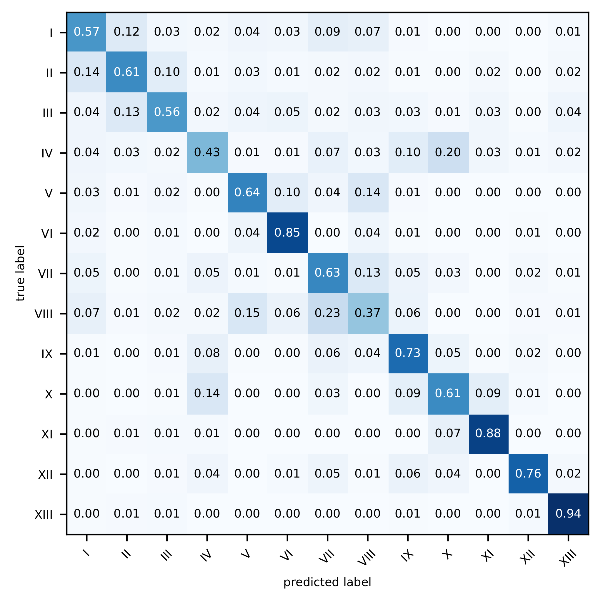
Figure 1. A visualisation of the workflow of the methodology. Input data is passed to the three experiments. CORINE is used in each experiment as ground truth for evaluating the predicted class labels arising from each experiment. Experiment 1 uses imagery and semantics, Experiment 2 uses semantics only, and Experiment 3 uses imagery only. For each experiment, a GSCM is created and an optimal deep learning model is identified before an accuracy assessment is made and the results of the three experiments are compared.
Remotesensing 13 03197 g001
Figure 2. A visualisation of the construction of a sample in the GSCM. The left side illustrates how geo-objects (dark red points) are used to calculate features for each OWL class, based on the azimuths (denoted as a) and distances (denoted as d) to them. On the right side of the figure, the scheme for the vectorization (dark blue arrow) of the imagery within the grid cell (red square) can be seen.
Remotesensing 13 03197 g002
Figure 3. The architecture of the optimal MLP model for Experiment 1 and 2 (upper figure) and Experiment 3 (lower figure).
Remotesensing 13 03197 g003
Figure 4. Confusion matrices for Experiment 1 and 2. (a) Confusion matrix of LULC classification of Experiment 1, using the fusion of semantics and imagery ( d m a x = 1 km). (b) Confusion matrix of LULC classification of Experiment 2, using semantics only ( d m a x = 1 km).
Remotesensing 13 03197 g004
Figure 5. Confusion matrix for using imagery only (Experiment 3).
Remotesensing 13 03197 g005
Figure 6. Three maps illustrating the geographic distribution of the errors of the three experiments: (a) for Experiment 1, (b) for Experiment 2 and (c) for Experiment 3. Each map shows grid cells of 1 km × 1 km which visualise the ratio of correctly classified samples within it. A ratio of 1.0 indicates that 100% of the samples within that cell were classified correctly. Two locations are marked in map (c). Location I corresponds to Lake Neusiedl; Location II corresponds to the region around mountain Grossglockner.
Remotesensing 13 03197 g006
Figure 7. Eight images showing cases, when a classification, based on semantics only (Experiment 2) worked correctly but not with imagery only (Experiment 3). (a) True class: Industrial, commercial, and transport units. Predicted class (imagery only): Mine, dump, and construction sites. (b) True class: Artificial, non-agricultural vegetated areas. Predicted class (imagery only): Mine, dump, and construction sites. (c) True class: Mine, dump, and construction sites. Predicted class (imagery only): Industrial, commercial, and transport units. (d) True class: Industrial, commercial, and transport units. Predicted class (imagery only): Mine, dump, and construction sites. (e) True class: Industrial, commercial, and transport units. Predicted class (imagery only): Mine, dump, and construction sites. (f) True class: Urban fabric. Predicted class (imagery only): Mine, dump, and construction sites. (g) True class: Artificial, non-agricultural vegetated areas. Predicted class (imagery only): Scrub and/or herbaceous vegetation associations. (h) True class: Permanent crops. Predicted class (imagery only): Urban fabric.
Remotesensing 13 03197 g007
Figure 8. Eight images showing cases when a classification, based on imagery only (Experiment 3), worked correctly but not with semantics only (Experiment 2). (a) True class: Industrial, commercial, and transport units. Predicted class (semantics only): Inland waters. (b) True class: Forests. Predicted class (semantics only): Scrub and/or herbaceous vegetation associations. (c) True class: Forests. Predicted class (semantics only): Arable land. (d) True class: Industrial, commercial, and transport units. Predicted class (semantics only): Urban fabric. (e) True class: Pastures. Predicted class (semantics only): Urban fabric. (f) True class: Industrial, commercial, and transport units. Predicted class (semantics only): Urban fabric. (g) True class: Forests. Predicted class (semantics only): Urban fabric. (h) True class: Urban fabric. Predicted class (semantics only): Arable land.
Remotesensing 13 03197 g008
Figure 9. Eight images showing cases, when a classification, based on semantics only (Experiment 2) as well as imagery only (Experiment 3), worked correctly. (a) True class: Forests. (b) True class: Forests. (c) True class: Industrial, commercial and transport units. (d) True class: Open spaces with little or no vegetation. (e) True class: Mine, dump, and construction sites. (f) True class: Urban fabric. (g) True class: Scrub and/or herbaceous vegetation associations. (h) True class: Industrial, commercial, and transport units.
Remotesensing 13 03197 g009
Figure 10. Eight images showing cases, when a classification, based on a fusion (Experiment 1) worked correctly but not on imagery as well as semantics alone (Experiment 2 and 3, respectively). (a) True class: Forests. Predicted class (imagery only): Artificial, non-agricultural vegetated areas. Predicted class (semantics only): Artificial, non-agricultural vegetated areas. (b) True class: Arable land. Predicted class (imagery only): Permanent crops. Predicted class (semantics only): Permanent crops. (c) True class: Pastures. Predicted class (imagery only): Heterogeneous agricultural areas. Predicted class (semantics only): Heterogeneous agricultural areas. (d) True class: Scrub and/or herbaceous vegetation associations. Predicted class (imagery only): Artificial, non-agricultural vegetated areas. Predicted class (semantics only): Artificial, non-agricultural vegetated areas. (e) True class: Urban fabric. Predicted class (imagery only): Pastures. Predicted class (semantics only): Pastures. (f) True class: Heterogeneous agricultural areas. Predicted class (imagery only): Forests. Predicted class (semantics only): Pastures. (g) True class: Urban fabric. Predicted class (imagery only): Heterogeneous agricultural areas. Predicted class (semantics only): Arable land. (h) True class: Arable land. Predicted class (imagery only): Heterogeneous agricultural areas. Predicted class (semantics only): Heterogeneous agricultural areas.
Remotesensing 13 03197 g010
Table 1. The 13 CORINE classes present in Austria. Please note, classes Sea water and Coastal wetland are not present, as Austria is landlocked. For each LULC class 12,000 samples were extracted.
CodeCLC Level 2 LULC Class
IUrban fabric
IIIndustrial, commercial, and transport units
IIIMine, dump, and construction sites
IVArtificial, non-agricultural vegetated areas
VArable land
VIPermanent crops
VIIPastures
VIIIHeterogeneous agricultural areas
IXForest
XScrub and/or herbaceous vegetation associations
XIOpen spaces with little or no vegetation
XIIInland wetlands
XIIIInland waters
Table 2. Overall accuracies (OA) and Kappa coefficients κ for different d m a x values, with the best results highlighted in bold.
Overall Accuracy (OA)
Semantics and Imagery (Experiment 1)
d m a x 20 [m]50 [m]500 [m]1 [km]5 [km]10 [km]30 [km]
OA [%]56.2254.4478.7882.1882.0681.1779.38
+/−1.520.570.380.290.310.210.24
Semantics only (Experiment 2)
OA [%]46.1242.4670.3076.1174.6073.1870.57
+/−1.010.930.510.250.50.30.44
Images only (Experiment 3)
OA [%]65.52
+/−0.44
KAPPA ( κ )
Semantics and imagery (Experiment 1)
20 [m]50 [m]500 [m]1 [km]5 [km]10 [km]30 [km]
κ 0.44120.47640.76990.80690.80560.79600.7766
+/−0.01490.00660.00410.00320.00310.00230.0026
Semantics only (Experiment 2)
κ 0.28680.33120.67800.74120.72480.70950.6810
+/−0.01400.01030.00560.00270.00540.00320.0047
Images only (Experiment 3)
κ 0.6264
+/−0.0047
Table 3. Training Parameters for all experiments. Experiment 1 and 2 share the same values. Experiment 3 has different values for the learning rate decay and the batch size.
ParameterExperiment 1 and 2 Experiment 3
OptimizerAdamaxAdamax
Learning rate (optimizer) 0.0010.001
Learning rate decay (optimizer) 8 × 10 7 5 × 10 7
ϵ (optimizer)1 × 10 9 1 × 10 9
β 1 (optimizer)0.9990.999
β 2 (optimizer)0.9990.999
Number of epochs12001200
Batch size20001000
Table 4. User’s and producer’s accuracy for Experiment 1 for each LULC class.
Producer’s Accuracy (Recall)Users’s Accuracy (Precision)
CLASS20 [m]50 [m]500 [m]1 [km]5 [km]10 [km]30 [km]20 [m]50 [m]500 [m]1 [km]5 [km]10 [km]30 [km]
I0.760.680.750.710.600.600.590.610.570.7140.740.750.710.65
II0.630.660.920.930.900.880.830.700.690.8790.890.880.870.86
III0.260.390.950.990.990.990.970.430.560.9230.950.930.930.92
IV0.440.530.900.960.960.950.920.550.610.8580.870.860.860.84
V0.190.350.610.660.690.690.660.300.380.7220.740.710.690.68
VI0.670.740.940.970.980.980.970.530.630.8240.860.870.870.85
VII0.250.430.630.660.690.650.640.420.420.6380.700.700.700.67
VIII0.240.310.500.580.610.580.550.270.310.5280.580.610.600.57
IX0.260.460.690.670.640.650.640.290.450.7440.780.780.770.76
X0.220.350.730.760.800.790.780.250.330.7260.770.750.750.74
XI0.480.600.880.900.900.890.880.530.610.8830.890.890.890.90
XII0.180.340.900.980.990.980.980.230.420.9020.940.930.920.91
XIII0.510.650.920.950.950.950.950.540.630.9430.950.960.960.95
Table 5. Producer’s accuracy (Recall) and user’s accuracy (Precision) for Experiment 2 (left side) as well as Experiment 3 (right side). For Experiment 2, the corresponding values for the different distance thresholds are shown. As Experiment 3 does not depend on this value, a single producer’s accuracy (left column denoted with P.A.) as well as user’s accuracy (right column denoted with U.A.) exists for each LULC class.
Producer’s Accuracy (Recall)User’s Accuracy (Precision) P.A.U.A.
CLASS20 [m]50 [m]500 [m]1 [km]5 [km]10 [km]30 [km]20 [m]50 [m]500 [m]1 [km]5 [km]10 [km]30 [km]CLASS
I0.790.700.690.580.290.240.210.510.490.720.760.750.720.60I0.570.57
II0.470.550.930.930.930.920.880.530.550.850.860.810.790.75II0.610.65
III0.150.250.971.001.001.001.000.310.360.880.920.900.890.86III0.560.69
IV0.360.450.910.960.960.960.950.340.480.850.860.830.820.78IV0.430.52
V0.090.150.430.590.600.580.540.260.260.550.630.590.580.54V0.640.65
VI0.480.570.900.960.980.970.950.360.410.790.850.840.830.81VI0.850.73
VII0.530.300.560.630.600.580.570.230.220.550.620.590.560.54VII0.630.51
VIII0.030.130.490.540.530.530.490.130.240.490.560.580.550.51VIII0.370.42
IX0.000.050.420.440.410.370.280.060.170.510.620.530.530.53IX0.730.63
X0.040.120.450.610.620.590.600.200.210.580.660.690.680.65X0.610.60
XI0.200.410.780.820.900.890.840.330.400.700.770.750.720.74XI0.880.82
XII0.100.140.870.970.980.980.970.280.350.760.860.900.880.84XII0.760.88
XIII0.130.190.780.880.910.910.890.450.390.780.820.810.790.77XIII0.940.87
Publisher’s Note: MDPI stays neutral with regard to jurisdictional claims in published maps and institutional affiliations.

