Stratified Particle Filter Monocular SLAM

Abstract

This paper presents a solution to the problem of simultaneous localization and mapping (SLAM), developed from a particle filter, utilizing a monocular camera as its main sensor. It implements a novel sample-weighting idea, based on the of sorting of particles into sets and separating those sets with an importance-factor offset. The grouping criteria for samples is the number of landmarks correctly matched by a given particle. This results in the stratification of samples and amplifies weighted differences. The proposed system is designed for a UAV, navigating outdoors, with a downward-pointed camera. To evaluate the proposed method, it is compared with different samples-weighting approaches, using simulated and real-world data. The conducted experiments show that the developed SLAM solution is more accurate and robust than other particle-filter methods, as it allows the employment of a smaller number of particles, lowering the overall computational complexity.

1. Introduction

After over two decades of extensive work, the robotics research community has proposed a multitude of advanced simultaneous localization and mapping (SLAM) approaches [1,2]. Solving the SLAM problem robustly is a necessary element to achieve full autonomy in the field of robotics. Among the most important elements of the simultaneous localization and mapping procedure, one can list surroundings perception with data extraction and association, robot pose estimation, local map building and maintaining global map coherence, so that the so-called loop closure can be performed in a previously visited area. A vast number of different solutions to all SLAM components has been proposed using numerous state-of-the-art frameworks. To classify different approaches, it is useful to categorize SLAM systems in accordance with the type of sensor used, the class of mathematical back-end synthesizing the pose and map information and the method of map representation.

A wide variety of sensors have been employed in SLAM: monocular cameras, stereo cameras, laser range finders, sonars, global positioning system (GPS) receivers, inertial measurement units (IMUs), etc. Some of those sensors can be used only for position estimation, others only to gather information about the environment, while devices such as cameras can be utilized for both purposes. The type of the chosen sensor determines the character of data that will be processed during the SLAM procedure, which influences subsequent stages of a SLAM framework design task.

The second vital aspect of the simultaneous localization and mapping, according to which different SLAM approaches can be distinguished, is the mathematical apparatus that is employed during the pose and map estimation step. For the sake of brevity, we will only address the basic distinction of filtering versus batch optimization. Filter methods characterize the map and the current pose information as a probability density function (PDF) using a variant of a Kalman filter (e.g., an extended Kalman filter (EKF) [3,4] or an unscented Kalman filter (UKF) [5]) or a particle filter (PF) [6,7]), a detailed description of which is presented later. A common feature of all filter methods is the lack of explicit storage of information about previous system states, which is commonly referred to as online or recursive state estimation. This stochastic modeling approach is referred to as the Markov chain. On the other hand, the optimization SLAM algorithms, known also as batch- or grid-based methods, perform a global or semi-global error minimization procedure from a set of previous poses and measurements. Also the keyframe-based SLAM should be mentioned here, as it is the most commonly used [2] optimization method for a visual SLAM. Keyframes are a small subset of distinctive camera frames recorded along the sensor trajectory. Only those characteristic keyframes are processed in the pose-map error minimization, which is performed using global bundle adjustment (BA) [8].

In [9], the authors proved that the optimization approach of the global BA approach offers better performance than the recursive filtering when comparing accuracy, computational complexity and robustness in large scale applications. However, the authors did not include a particle filter method in their testing, justifying the omission by an assumption that it is wasteful to employ a particle filter for unimodal distributions estimation. However, categorizing the SLAM procedure, where an algorithm has to evaluate not only the robot or sensor pose but also the state of rarely static surroundings, as a strict unimodal distribution estimation can be considered an oversimplification. Particle filters provide a more robust, multimodal modeling approach. Moreover, PFs computational complexity, contrary to Kalman filters, does not scale cubically [10] in terms of the number of observed landmarks. It is linear—similar to batch SLAM algorithms. Therefore, we consider particle filters as a valid and reasonable solution to the concurrent localization and mapping problem.

Another useful means of the classification of SLAM methods is the map building approach, which can be done using two separate but interdependent criteria. To begin with, the map can be built either directly or indirectly. The first method is based on analyzing the surroundings using unprocessed sensor readings, while the latter identifies specific features in the environment according to a chosen extraction approach, which can be different geometric shapes (e.g., points [11], corners [12] and lines [13]) or more complex objects [14]. The way that the map elements are picked is directly associated with the resulting map type. A given SLAM procedure can produce either a dense map of the environment where every part of an observed area—for example every registered pixel—is associated with a distinct element of the map. This approach is commonly used in SLAM systems that utilize sensors which are capable of determining full three-dimensional measurements of the environment, like rangefinders [15] or RGBD cameras [16]. On the other hand, the registration of a sparse map is a process wherein the map is constructed around salient scene elements (characteristic points, regions or shapes), that can be correctly associated in subsequent sensor observations.

As different reviews show [1,17,18], although the development of SLAM systems offers a wide range of opportunities for modern autonomous systems, the simultaneous localization and mapping domain has yet to achieve complete success. Hence, the community needs to address various potential solutions to concurrent localization and mapping problems. Our manuscript presents a novel framework for an indirect, monocular SLAM, based on a Rao–Blackwellized particle filter. We incorporate a distinctive approach towards particle weighting, where the weights are stratified proportionally to the number of landmarks matched in a given camera frame. This approach offers better accuracy and robustness than standard resampling methods. Thus, it allows to lower the computational complexity of the SLAM algorithm by decreasing the number of particles needed for adequate performance. Furthermore, our algorithm has been examined using both simulation and real-world data, registered from a quadcopter. The presented approach was tested in various set-ups and all the results were consistent. The paper contains selected results of the simulations and experiments. The remainder of this article is outlined as follows: In Section 2, the related work in the field of particle filter SLAM is discussed; in Section 3, a detailed explanation of the proposed algorithm is presented; simulation and real experimental results are provided in Section 4 to validate the adopted approach. The conclusions of the paper are included in Section 5. This manuscript is a continuation of our previous works in the field of particle filter SLAM [19] but offers a new approach to the filtering algorithm.

2. Related Work

The earliest idea of a SLAM framework employing a Rao–Blackwellized particle filter was briefly discussed in [20]. The authors advocated the use of Bayesian inference in order to achieve autonomous localization and mapping capabilities. Undoubtedly, the most well-known solution to a Rao–Blackwellized particle filter SLAM was presented in [6], where lidar was used to build a grid map. Many later systems have been designed upon FastSLAM (both 1.0 and 2.0 [7]) frameworks—especially those utilizing rangefinders as main sensors [21,22,23].

Rapid progress in computer vision and computational capacity led to the proliferation of cameras in the field of robotics. Among the first systems that employed a particle filter and a camera to perform simultaneous localization and mapping, one should list [24]. The algorithm described in that manuscript processed edges, found with the Sobel mask, as landmarks, but did not benefit from the fact that different observations can be treated as probabilistically independent if one knows the camera position and orientation. As a result, 10,000 particles had to be used to estimate the state of the camera pose, together with only 15 landmarks. In [25], the authors implemented an algorithm that allowed one to sequentially approximate the full 6DoF posterior of a camera, together with up to eight, tracked 3DoF scene points. This method was successfully validated using 500 particles; however, a small set of previously known landmarks was required for it to work properly. Another system, developed by Sim et al. [26], is an early example of a Rao–Blackwellized particle filter framework that was constructed using a camera as the main sensor. With the usage of the SIFT algorithm [27], the authors’ indoor mobile robot was able to successfully track more than 11,000 landmarks. Later, Eade and Drummond [15] constructed an algorithm capable of camera-tracking with as little as 50 particles and implemented the ingenious idea of inverse depth [28] as a third element of a 3DoF landmark-state vector. In [29], the authors extracted landmarks using speeded-up robust features (SURF) [30] and applied a global optimization algorithm to achieve optimal matching for its scene points.

While the earliest formulations of Rao–Blackwellized particle filters in a FastSLAM-like framework assumed that map elements are estimated using EKFs, other monocular SLAM approaches implemented alternative nonlinear Kalman filtering strategies, namely the UKF. In [31], the authors exploited the spatial structure of the environment and developed an algorithm that searched for and extracted locally planar objects as landmarks, whilst Lee [32] introduced a template prediction mechanism to compensate for camera motion. Both mentioned systems employed UKFs for landmark storage to overcome the issue concerning Jacobians approximations in EKFs.

The profound analysis presented in [9] marked a milestone in the SLAM systems domain, as more researchers have tended to shift towards keyframe simultaneous localization and mapping approaches over the last decade. Still, there have been numerous examples of efficient PF SLAM methods implemented since. One of them was proposed in [33] as a tool for pose-tracking for augmented reality. The algorithm implemented an idea to discard outliers indirectly—not during the data association-and-gating phase but after the particle-weighting procedure, as incorrect matches lower sample weights significantly, thus minimizing chances for a given particle to be resampled. The authors used both lines and points, extracted with a Harris corner detector [34] and Hough line transform, respectively. A different particle filter-based solution to the SLAM problem was outlined in [35] for an indoor aerial vehicle. Asserting that the robot was designed to navigate only inside manmade structures, that system exploited the abundance of straight lines in the camera images and facilitated human-like procedures to predict landmark depths. The ranging strategy assumed that the monocular camera altitude was known, and used this information to process relative poses of observed geometric structures in order to synthesize a simultaneous localization-and-mapping algorithm, similar to the FastSLAM approach.

As mentioned before, the monocular camera-observation model suffers greatly from a lack of depth information. Contrary to monocular-camera algorithms, RGBD-camera-based-SLAM approaches are able to directly initialize landmark depths using single-sensor reading. One paper [36] presents a remarkable stereo-camera-particle-filter-SLAM solution, where the authors proposed a smart procedure for outlier identification by landmark-position correlation analysis. Moreover, landmarks are efficiently detected and matched using the SURF algorithm. To tackle the unknown depth issue otherwise, one can place a pattern of known dimensions inside the camera field of view. In [37], the authors proposed the insertion of a chessboard inside the first few camera frames to allow an accurate depth estimation as well as a reduction of camera pose uncertainty for a monocular-camera-based SLAM system. To calculate the depth of subsequently observed landmarks, the described algorithm delayed their initialization until a triangulation procedure could be carried out.

In reference to SLAM being strictly a perception problem, one would intuitively seek its refinement in the modification of a given observation model. However, Zhou and Maskell proposed an improvement to the FastSLAM framework based on the motion model revision. In [38], the estimation of system dynamics is partitioned into two sub-models. The camera location was calculated with a particle filter, and its velocity with a Kalman filter. This idea allowed one to reduce the particle filter’s dimensionality, as well as to achieve a better accuracy than one would with an analogous solution constructed upon the classic FastSLAM framework.

Further examples of particle-filter SLAMs also include non-pure-visual systems, where data from range finders are fused with images. Chen et al. [39] implemented a system wherein an urban search-and-rescue robot navigates using 2D lidar in a feature-based 3D map, constructed with a monocular camera. This allows for the obtaining of a real scale of the surroundings, as well as the maintenance of full, 6DoF motion and mapping capabilities. In [40], the authors propose a system wherein one robot performs the camera SLAM while others reuse the resulting map for simultaneous localization-and-map-scale estimation.

Among additional instances of PF-based systems in the field of robotics, recent works not related directly to the SLAM problem should be listed as well. The manuscript by Acevedo et al. [41] characterizes an algorithm which employs a particle filter to enable a group of networking robotic entities to search for a moving target. In [42], PF is used as a framework to solve 6DoF, visual pose-tracking, where Rao–Blackwellization is introduced by decoupling the translation and orientation data. In a paper by Di Yuan et al. [43], a PF-based system for redetection in the object-tracking approach for accurate localization in difficult conditions is described. In [44], the authors describe a self-localization technique that employs a PF, based on particle swarm optimization, that requires fewer particles to function correctly than comparable benchmark approaches.

3. Materials and Methods

Although the method that we propose in this paper can be easily adjusted to any monocular camera configuration, our SLAM framework was designed and validated under the assumption it will serve as a secondary navigational system for a surveillance UAV with its monocular camera pointed downward. Based on inertial-measurement-unit (IMU) measurements and subsequent camera frames, we were able to synthesize the registered data into a correct trajectory, together with a sparse map of the observed area.

3.1. Motion Model

To minimize the number of reference frames needed, our system directly estimates the pose (position and orientation) of a camera sensor, rather than the pose of a UAV itself. The state vector $x_k$ during time step $k$ consist of nine variables:

$$x_k=\left[\begin{array}{c}x\\ \begin{array}{c}y\\ \begin{array}{c}\begin{array}{c}\begin{array}{c}\begin{array}{c}z\\ v_x\end{array}\\ v_y\end{array}\\ v_z\end{array}\\ \begin{array}{c}\varphi \\ \begin{array}{c}\theta \\ \psi \end{array}\end{array}\end{array}\end{array}\end{array}\right]$$

(1)

where $x$, $y$, $z$ represent a localization in Cartesian coordinates, $v_x$, $v_y$, $v_z$ are orthogonal components of a velocity vector and $\varphi$, $\theta$ and $\psi$ are the roll, pitch and yaw orientation angles respectively. We choose the east-north-up (ENU) coordinate system as the global reference frame, where $x$ is east, $y$ is north and $z$ is up. The source of camera orientation, relative to the ENU frame, is obtained from the onboard IMU.

While the camera itself has six degrees of freedom (6DoF), the bearing-only observation model causes monocular SLAM to be a 7DoF problem, where a map representation can be determined only up to a scale. To mitigate the issue of scale ambiguity and drift, which is an inherent problem of single-camera SLAM frameworks, we chose to select the onboard IMU as an additional sensor. It is used as the source of a stream of metric measurements that are control signals for trajectory prediction. The employment of an inertial measurement unit implicates the usage of a constant velocity (CV) motion model as the most appropriate. The discretized motion equation describing the camera movement relationships is given below:

$$x_k=f\left(x_{\mathrm{k}-1},u_{\mathrm{k}}\right)+w_k$$

(2)

where $x_{\mathrm{k}}$ is the predicted state vector containing estimates of the platform’s kinematic parameters, $x_{\mathrm{k}-1}$ is the state vector estimated during the previous time step $k-1$, $f$ is the state-transition nonlinear vector function, $u_k$ represents IMU readings, and $w_k$ is the additive Gaussian process noise which can be described by a zero-mean multivariate normal distribution $N\left(0,Q_k\right)$ where $Q_k$ denotes the process covariance matrix.

3.2. Sensor Model

As previously stated, a single camera is the main sensor utilized for map building in our SLAM system. Monocular cameras are common components of off-the-shelf UAVs. Among their advantages which can be considered the most beneficial in the field of robotics are their small size and low cost, as well as low power consumption. Moreover, the update rates and resolutions of these cameras are sufficient to track environmental changes during motion at velocities up to tens of meters per second. These features are the reason that monocular cameras are widely used for localization, structure from motion, mapping, SLAM etc. However, one can also identify consequential drawbacks of the single-camera usage. The main disadvantage, which has to be addressed when analyzing the monocular sensor model, is the lack of depth information. In other words, the perspective projection that transforms 3D real-world points into 2D camera pixels coordinates is lossy and causes a pose calculation problem for extracted real-world features. As landmark 3D positions cannot be straightforwardly computed, the approach to resolve this difficulty needs to be adopted. To address this issue, a given algorithm can either initialize a landmark immediately after its first observation (where the uncertainty of measured depth is set as significantly larger than for other coordinates), or delay the feature detection until observations from different perspectives provide conditions for temporal view stereoscopy analysis, to estimate information about the landmark’s full, 3D pose. The first approach is called an undelayed initialization, while the latter is commonly referred to as delayed landmark initialization.

The adopted sensor model, together with the initialization strategy, starts with a single-camera frame registration. The camera’s intrinsic parameters are known and can be denoted as $K_{intr}$:

$$K_{intr}=\left[\begin{array}{ccc}{f}_x& s& u_0\\ 0& f_y& v_0\\ 0& 0& 1\end{array}\right]$$

(3)

where $f_x$ and $f_y$ represent focal lengths along the camera’s axis and are equal for a pinhole camera model, $u_0$ and $v_0$ are principal point offset and $s$ is the camera axis skew.

To extract distinctive scene points from images, we use the SURF algorithm [21]. The SURF detector outputs a set of pixel coordinates in a given image frame, where the determinant of a Hessian matrix reaches its maximum value. It is worth noting that SURF points are scale and rotation invariant. Exemplary extraction procedure results are presented in Figure 1.

To represent extracted scene points in the ENU coordinate frame, we use the concept of anchored modified-polar points, which can also be referred to as inverse-distance points (IDP) [45]. A single IDP point is defined by a six-element vector:

$${}^{p}m_k^i=\left[\begin{array}{c}\begin{array}{c}{x}_0\\ y_0\\ z_0\end{array}\\ \begin{array}{c}\epsilon \\ \alpha \\ \rho \end{array}\end{array}\right]$$

(4)

where ${}^{p}m_k^i$ is the state of the $i$-th landmark observed by the $p$-th particle at the time $k$. The first three elements of the state vector ($x_0$, $y_0$, $z_0)$ are the ENU coordinates that encode the position of the particle from which the landmark was originally observed (the point ${}^{p}p_0$ in Figure 2.). These coordinates are frequently referred to as the anchor point. Next, $\epsilon$ and $\alpha$ are respectively the elevation and azimuth angles at which the observation was made, while $\rho =\frac{1}{d}$ is the inverse of the distance between the camera and the scene point.

Figure 2 presents the idea of IDP landmark parametrization. The usage of anchored modified-polar points allows one to initialize landmarks in the map immediately. Still, the monocular-camera, salient-feature extraction step provides only two-dimensional measurements of three-dimensional objects’ locations, where the distance $d$ remains unknown. To resolve the issue of being unable to recover the true localization of the environment features, we choose the strategy of setting an initial inverse depth, of every registered landmark, as a preset value with reasonably large uncertainty. As the camera is pointed downwards, the starting depth value is either assumed equal to the UAV’s altitude or is calculated using positions of nearby, previously seen scene points. The standard deviation of such observation is selected in a way so as to include infinite distance (inverse depth equal to 0) in the $3\sigma$ region. Using the undelayed initialization scheme allows one to comply with the adopted discrete-time Markov chain approach, and satisfies the property of a memoryless process, such that the currently processed state is sufficient to estimate the probability distribution of future states.

The first step of the initialization of a newly observed landmark is to transform its coordinates, expressed in pixels of the image plane, using the pinhole camera model. The inverse camera projection is performed in accordance to the equation below:

$$\left[\begin{array}{c}{x}_{cam}\\ y_{cam}\\ 1\end{array}\right]=K_{intr}{}^{-1}\left[\begin{array}{c}u\\ v\\ 1\end{array}\right]$$

(5)

where $u$ and $v$ are pixel coordinates in a registered image frame while $x_{cam}$ and $y_{cam}$ are coordinates in the standard reference frame of the camera. Next, by transforming the resultant vector so that it is expressed in the global reference frame (ENU), the optical ray pointing from the camera center ${}^{p}p_0$ to the extracted scene point is obtained:

$$\left[\begin{array}{c}{x}_{enu}\\ y_{enu}\\ z_{enu}\end{array}\right]={}^{enu}R_{cam}\left[\begin{array}{c}{x}_{cam}\\ y_{cam}\\ 1\end{array}\right]$$

(6)

where ${}^{enu}R_{cam}$ encodes the rotation from the camera reference frame to ENU coordinates. The usage of IDP parametrization implies the lack of need for the employment of 3D coordinates in a homogeneous form, as the obtained vector is subjected only to rotation. The information that is conventionally contained in translation—when using 3D Euclidean points as landmark representation—is encoded in the anchor point ${}^{p}p_0$.

Next, the vector’s ENU coordinates are expressed using a modified-polar point convention:

$$\left[\begin{array}{c}\epsilon \\ \alpha \\ \rho \end{array}\right]=\left[\begin{array}{c}atan2\left(z_{enu},\sqrt{x_{enu}{}^2+y_{enu}{}^2}\right)\\ atan2\left(y_{enu},x_{enu}\right)\\ \frac{1}{d}\end{array}\right]$$

(7)

where $\epsilon$ and $\alpha$ are respectively the elevation and yaw angles and $\rho$ is the inverse depth. The addition of the anchor point results in the acquiring of the complete IDP landmark parametrization:

$${}_{}{}^{p}m_k^i=\left[\begin{array}{c}{}^{p}p_0\\ \begin{array}{c}\epsilon \\ \alpha \\ \rho \end{array}\end{array}\right]=\left[\begin{array}{c}\left[\begin{array}{c}{x}_0\\ y_0\\ z_0\end{array}\right]\\ atan2\left(z_{enu},\sqrt{x_{enu}{}^2+y_{enu}{}^2}\right)\\ \begin{array}{c}atan2\left(y_{enu},x_{enu}\right)\\ \frac{1}{d}\end{array}\end{array}\right]$$

(8)

As landmarks are stored using separate EKFs, the initialization procedure has to comprise the calculation of the landmark covariance matrices as well. A covariance matrix ${}_{ }{}^{p}P{}_k^i$ that describes the uncertainty of a transformation of the 2D point extracted from an image frame to its IDP representation is given by the following formula:

$${}_{ }{}^{p}P{}_k^i={\left({}_{ }{}^{p}H{}_k^i\right)}^{-1}{R}_k^p{\left[{\left({}_{ }{}^{p}H{}_k^i\right)}^{-1}\right]}^T+\left[\begin{array}{ccc}\begin{array}{c}\begin{array}{cc}0& 0\end{array}\\ \begin{array}{cc}0& 0\end{array}\end{array}& \begin{array}{c}\begin{array}{cc}0& 0\end{array}\\ \begin{array}{cc}0& 0\end{array}\end{array}& \begin{array}{c}\begin{array}{cc}0& 0\end{array}\\ \begin{array}{cc}0& 0\end{array}\end{array}\\ \begin{array}{c}\begin{array}{cc}0& 0\end{array}\\ \begin{array}{cc}0& 0\end{array}\end{array}& \begin{array}{c}\begin{array}{cc}0& 0\end{array}\\ \begin{array}{cc}0& 0\end{array}\end{array}& \begin{array}{c}\begin{array}{cc}0& 0\end{array}\\ \begin{array}{cc}0& 0\end{array}\end{array}\\ \begin{array}{c}\begin{array}{cc}0& 0\end{array}\\ \begin{array}{cc}0& 0\end{array}\end{array}& \begin{array}{c}\begin{array}{cc}0& 0\end{array}\\ \begin{array}{cc}0& 0\end{array}\end{array}& \begin{array}{c}\begin{array}{cc}0& 0\end{array}\\ \begin{array}{cc}0& {\sigma }_{\rho }^2\end{array}\end{array}\end{array}\right]$$

(9)

where $R_k^p$ is a two-by-two sensor-noise matrix, describing the accuracy of the scene point localization in the image plane, and ${\left({}_{ }{}^{p}H{}_k^i\right)}^{-1}$ follows the ordinary EKF notation and denotes a Jacobi matrix of the inverse observation function that describes the transformation from pixel coordinates to the ENU coordinate system. ${\left({}_{ }{}^{p}H{}_k^i\right)}^{-1}$ is given by the following formula:

$${\left({}_{ }{}^{p}H{}_k^i\right)}^{-1}=\left[\begin{array}{c}\begin{array}{ccc}0& 0& 0\\ 0& 0& 0\\ 0& 0& 0\end{array}\\ \begin{array}{ccc}1& 0& 0\\ 0& 1& 0\\ 0& 0& 1\end{array}\end{array}\right]{}_{ }{}^{p}J{}_k^i{}^{enu}R_{cam}{K}_{intr}{}^{-1}\left[\begin{array}{cc}1& 0\\ 0& 1\\ 0& 0\end{array}\right]$$

(10)

where ${}^{p}J_k^i$ is the Jacobi matrix of a function that transforms the vector pointing from the ${}^{p}p_0$ to the $i$-th landmark from 3D ENU Cartesian coordinates into modified spherical coordinate system representation and is equal to:

$${}^{p}J_k^i=\left[\begin{array}{ccc}\frac{x_{enu}{z}_{enu}\left(x_{enu}{}^2+y_{enu}{}^2+z_{enu}{}^2\right)}{-\sqrt{x_{enu}{}^2+y_{enu}{}^2}}& \frac{y_{enu}{z}_{enu}\left(x_{enu}{}^2+y_{enu}{}^2+z_{enu}{}^2\right)}{-\sqrt{x_{enu}{}^2+y_{enu}{}^2}}& \frac{\sqrt{x_{enu}{}^2+y_{enu}{}^2}}{x_{enu}{}^2+y_{enu}{}^2+z_{enu}{}^2}\\ \frac{-y_{enu}}{x_{enu}{}^2+y_{enu}{}^2}& \frac{x_{enu}}{x_{enu}{}^2+y_{enu}{}^2}& 0\\ 0& 0& 0\end{array}\right]$$

(11)

During camera movement, in subsequent time steps, the sensor model is able to retrieve the bearings of extracted features from consecutive, multiple views. The SLAM algorithm gradually estimates real 3D poses of landmarks, using standard EKF update equations given below:

$${}^{p}y_k^i=z_k^{\left[i\right]}-h\left({}^{p}m_k^{\left[i\right]}\right)$$

(12)

$${}^{p}S_k^{\mathrm{i}}={}^{p}H_k^{\mathrm{i}}{}^{p}P_{k-1}^{\mathrm{i}}{\left({}_{ }{}^{p}H{}_k^{\mathrm{i}}\right)}^T+R_k^p$$

(13)

$${}_{ }{}^{p}K{}_k^i={}_{ }{}^{p}P{}_{k-1}^{\mathrm{i}}{\left({}_{ }{}^{p}H{}_k^{\mathrm{i}}\right)}^T{\left({}_{ }{}^{p}S{}_k^{\mathrm{i}}\right)}^{-1}$$

(14)

$${}^{p}m_{k+1}^i={}^{p}m_k^{\mathrm{i}}+{}_{ }{}^{p}K{}_k^i{}^{p}y_k^i$$

(15)

$${}_{ }{}^{p}P{}_k^{\mathrm{i}}=\left(I_{6x6}-{}_{ }{}^{p}K{}_k^i{}_{ }{}^{p}H{}_k^{\mathrm{i}}\right){}_{ }{}^{p}P{}_{k-1}^{\mathrm{i}}$$

(16)

where ${}^{p}y_k^i$ is the measurement innovation (of the $i$-th landmark seen by the $p$-th particle), $z_k^{\left[i\right]}$ is the measurement itself and $h$ is the nonlinear vector function that describes the projection of a predicted scene point location from the 3D ENU coordinates to the image plane. It is the inverse of the transformation described in the Equation (5) through (11). Furthermore, ${}^{p}S_k^{\mathrm{i}}$, ${}^{p}H_k^{\mathrm{i}}$ and ${}^{p}K_k^i$ are respectively the residual covariance, the Jacobian of the vector function $h$, and the Kalman gain—calculated for a given particle-landmark pair—during time step $k$.

3.3. Sequential Importance Resampling (SIR) Particle Filter

A particle filter is a mathematical tool capable of the accurate estimation of non-linear, non-Gaussian and multimodal distributions. Among different PF variants, the sequential importance resampling (SIR) approach is suited best for SLAM applications, and most of the previously mentioned works use it to address the simultaneous localization on the mapping problem. Our SLAM algorithm is built upon a SIR PF as well. The filtering operation is conducted by drawing a weighted set of samples that are generated in accordance with a predefined distribution from a set of particles from a previous time step. To address the issue of a particle filter degeneracy, a resampling procedure is run periodically to exclude samples with the lowest weights—i.e., less probable hypotheses.

To achieve a robust and efficient filtering procedure, the proposal’s distribution of samples has to match the desired distribution as closely as possible. Therefore, particles representing poses of the camera are sampled at a frequency equal to the IMU data sample rate. This process is performed in accordance to the motion model described by Equation (2), and its PDF is assumed to be in the following form:

$$p\left(x_k|x_{k-1},u_k\right)$$

(17)

Performing SLAM, rather than simple navigation, indicates the inclusion of a set of extracted landmarks in the filtering process. The straightforward approach of recovering the momentary camera pose and the map of its surroundings with a particle filter is given by the joint posterior:

$$p\left(x_k,m_k^{\left[1:M\right]}|x_{k-1},u_k,z_k\right)$$

(18)

where $m_k^{\left[1:M\right]}$ is a set of all $M$ landmarks observed up to time $k$. The number of particles required to estimate the PDF accurately grows exponentially, as every newly added landmark increases the number of dimensions of the state space that has to be sampled. Therefore, for SLAM systems designed to navigate robustly and effectively through large areas, a change in this approach is necessary. To solve the issue of a rapid increase of the number of required particles, PF SLAM systems commonly benefit from the fact that the estimations of observed scene points can be treated as conditionally independent, if the robot trajectory is assumed to be known. The application of this relationship results in a special case of the Rao–Blackwellization (RB) of a particle filter and is based on marginalizing landmarks out of the state vector [20]. The standard RB PF is the mathematical basis of the adopted SLAM framework. The consequence of state-vector size reduction is a decrease in the number of samples needed to perform a SLAM routine accurately. The resulting joint posterior is:

$$p\left(x_k,m_k^{\left[1:M\right]}|x_{k-1},u_k,z_k\right)=p\left(x_k|x_{k-1},u_k\right)p\left(m_k^{\left[1:M\right]}|x_k,z_k\right)$$

(19)

and can be further factored out as:

$$\left(x_k,m_k^{\left[1:M\right]}|x_{k-1},u_k,z_k\right)=p\left(x_k|x_{k-1},u_k\right){\displaystyle \prod }_{\mathrm{i}=1}^M\left(m_k^{\mathrm{i}}|x_k,z_k\right)$$

(20)

The implementation of this conceptual solution to Rao–Blackwellized SLAM is performed by the division of the estimation task among different filters. The main particle filter models the camera trajectory with a number of weighted samples, while landmark positions are estimated using EKFs, whose accuracy determine particle weights. Every particle has to maintain a separate EKF for every observed scene point. This implicates the computational complexity of $O\left(MN\right)$ for $N$-particle distribution, describing the pose of a camera and an $M$-landmark map.

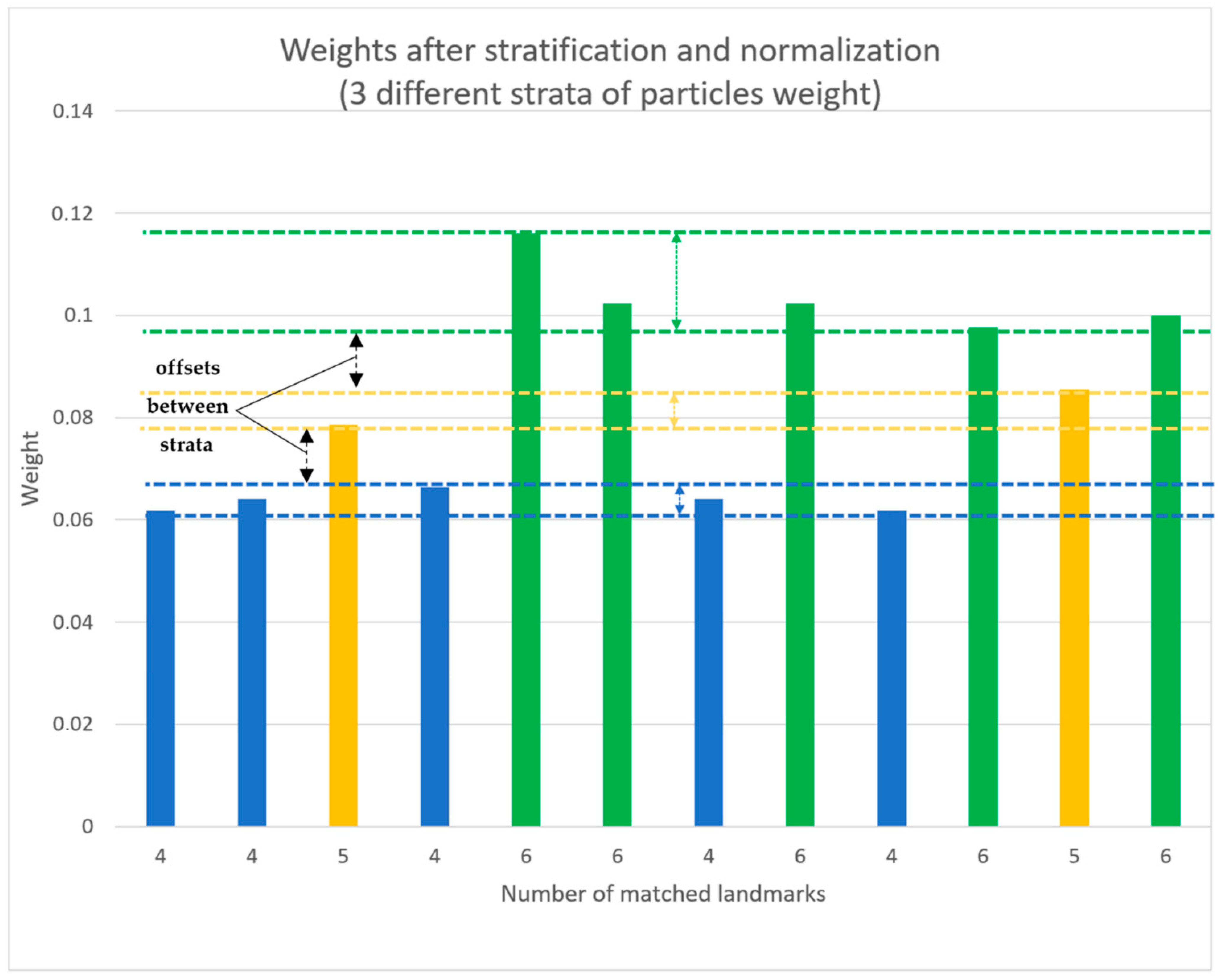
3.4. Weighting Approach

The samples in a particle filter are weighted according to the likelihood functions that describe the accuracy of camera readings, given the predicted landmarks and sensor locations. The weight of a particle is inversely proportional to the innovation of observed landmarks $y_k^{\left[1:L_k^p\right]}$ in a time step $k$ which is measured in pixels, in the image frame:

$$w_k^p~w_{k-1}^{p}p\left(y_k^{\left[1:L_k^p\right]}|x_k^{\left[p\right]}\right)$$

(21)

where $L_k^p$ is the number of landmarks matched by the particle $p$ at a time $k$. The weight of a given particle can be further calculated using the following formula:

$$w_k^p=w_{k-1}^p{\left|2\pi S_k^{\left[1:L_k^p\right]}\right|}^{-1/2}exp\left[-\frac{1}{2}{\left(y_k^{\left[1:L_k^p\right]}\right)}^T{\left(S_k^{\left[1:L_k^p\right]}\right)}^{-1}{y}_k^{\left[1:L_k^p\right]}\right]$$

(22)

where $S_k^{\left[1:L_k^p\right]}$ is the innovation covariance matrix constructed for all landmarks that were matched with the previously seen scene points at a time step $k$. The particle cloud encoding exemplary estimates in a particle filter in the local body frame is shown in Figure 3.

For our algorithm to include particular landmarks in the sample-weight calculation, they have to be correctly associated with previously extracted scene points. The matching procedure consists of two steps. After the visual association of image features, which is based on a comparison of SURF descriptors (and was described in previous sections), we proceed to spatial gating, using the Mahalanobis distance to remove spatial outliers. This step introduces a potentially error-prone dependency. Namely, landmark matches have to be gated in accordance with measurement residuals $y_{k+1}^{\left[i\right]}$ for all the potential associations—for every particle. As the set of samples represents the complete PDF of a camera pose, the differences between predicted and observed landmark positions vary between particles, while the matching threshold remains constant. Consequently, the number of landmarks that pass the gating criterion may differ within the particle set. Hence, using the Mahalanobis distance as a straightforward solution to the outliers issue introduces distinctive ambiguities during the particle weighting and resampling procedures. While every observation is assumed to be independent and normally distributed, Equation (22) could be rewritten as:

$$w_k^p=w_{k-1}^p{\displaystyle \prod }_{i=1}^{L_k^p}{\left|2\pi S_k^{\left[i\right]}\right|}^{-1/2}exp\left[-\frac{1}{2}{\left(y_k^{\left[i\right]}\right)}^T{\left(S_k^{\left[i\right]}\right)}^{-1}{y}_k^{\left[i\right]}\right]$$

(23)

The magnitude of $y_{k+1}^{\left[1:L_k^p\right]}$ depends on the deviation from the true trajectory of the camera for a given particle. Due to the nature of the computation and system parameters, every product factor of the resulting weight $w_k^p$ is significantly smaller than one. Thus, every matched landmark $1:L_k^p$ causes $w_k^p$ to decrease. Consequently, although the number of matched landmarks is, in general, proportional to the accuracy of the trajectory estimation process, it is not unusual that, for two given particles whose poses resulted in matching a different number of landmarks, the one with more matches would have a lower importance factor. This is caused by the gating step, as the negative impact of the magnitudes of landmark-pose innovations on $w_k^p$ is often lesser than the presence of additional product factors. A natural way to include the missed landmarks in the weight calculation would be to introduce a probability of incorrect association $P_{ia}$ into the Equation (23):

$$w_k^p=w_{k-1}^p{\left(1-P_{ia}\right)}^{L_k^p}{\displaystyle \prod }_{i=1}^{L_k^p}{\left|2\pi S_k^{\left[i\right]}\right|}^{-1/2}exp\left[-\frac{1}{2}{\left(y_k^{\left[i\right]}\right)}^T{\left(S_k^{\left[i\right]}\right)}^{-1}{y}_k^{\left[i\right]}\right]P_{ia}{}^{L_{max}-L_k^p}$$

(24)

where $L_{max}$ is the maximum number of matched landmarks by any of the particles during a given time step. The tested value of $P_{ia}$ ranged between 0.2 and 0.001 [46]. However, simulations shown in the next section suggest that this idea is insufficient to solve the beforementioned problem—the weights of particles which matched fewer landmarks were often still larger, as the sole adjustments of the $P_{ia}$ did not allow one to tune the weighting process accurately. To efficiently address this issue, we introduce the weight stratification scheme. The idea behind this approach is based on adopting the number of matched landmarks as a primary importance factor criterion. After initial weighting, samples are divided into subsets according to the number of correctly matched scene points and their weights are further adjusted. The adjustment is performed with the addition of offsets to particle weights in a way that separates each of the subsets, creating disjunctive strata of particles. The details of the stratification algorithm are described in the flowchart presented in Figure 4. The graphical interpretation of this procedure is illustrated in Figure 5 and Figure 6. In this way, matching more landmarks by a given particle guarantees having a greater weight.

The offset that separates the strata is equal to the following expression:

$$\mathit{offset}=\left(L_{\max }-L_k^s\right)\ln P_{ia}$$

(25)

where $L_k^s$ is the number of landmarks matched by particles in a given strata $s$.

Applying the algorithm results in the stratification of sample subsets. Of note is the fact that the procedure is performed in such a manner that particle-weight ratios, in distinct subsets, are preserved. The weights adjustment outcome is presented in the figures below.

After the stratification and normalization, the system performs the resampling procedure, though only if the efficient number of particles $N_{eff}$, calculated using the expression below, is less than a quarter of the true number of particles.

$$N_{eff}=\frac{1}{{\sum }_{p=1}^N{\left(w^p\right)}^2}$$

(26)

This procedure allows one to replace samples of negligible weights with those representing the most probable state hypotheses only when significant disproportions in particle weights occur.

3.5. Landmark Management

To perform large scale simultaneous localization and mapping, a SLAM architecture has to address the issue of efficient landmark management. Particle-filter solutions are especially vulnerable to rapid increases in the number of scene points used for mapping, as every particle represents a unique map. Our SLAM system manages landmarks in a way that minimizes memory usage. To achieve it, we run two separate data sets. One of them stores landmark data that is shared among all particles, such as scene-point coordinates in an image frame, their SURF descriptors, and information on whether landmarks were identified in the currently processed frame and if they were newly observed. Furthermore, a unique ID is assigned to every scene point in the first set. The other database contains information that can be referred to as particle-dependent: landmark positions, covariance matrices, SURF-matching and Mahalanobis-gating results, the number of times landmarks were seen and updated, as well as the number of times landmarks were not observed if their pose indicated otherwise, last-observation and update times, the last angle of observation and the observation-likelihood values.

Furthermore, robust operation requires a flexible approach to landmark initialization and removal. The algorithm distinguishes four different states in which a landmark can be after the data-association procedure. First, a new landmark is extracted and initialized if the number of matched landmarks in the current frame is lower than the predefined threshold of a desired number of landmarks per frame. This prioritizes already-seen scene points over newly observed ones. In addition, scene points that were matched correctly are further examined in terms of angle of observation. If the angle between the current camera pose and the pose of the sensor during the last landmark observation is larger than a predefined threshold, which provides sufficient triangulation conditions, the landmark is updated, using EKF. Otherwise, the landmark is only marked as matched. This artificial limitation of landmark-update frequency is necessary, due to the properties of the EKF covariance-matrix-update equation. If a landmark is not observed, even though it is predicted to be inside the current sensor Field of View (FOV), it is marked as unmatched. After processing all observations, the variables that monitor the number of updates, correct matches and failed observations are updated for all particles and their associated scene points.

The last part of landmark management is landmark removal. The removal assessment is based on the algorithm described by the flowchart in Figure 7 and performed particle-wise.

Only after a given landmark is removed by all of the particles is its data in the dataset shared among deleted particles as well.

In terms of accuracy, it is more useful to increase the number of scene points, rather than the number of processed image frames per second [9]. Hence, we adjusted our system such that the frames-per-second rate is artificially lowered to less than five, so that the number of extracted, associated and initialized features during every frame could be maximized without increasing the computational burden.

Each loop of the presented particle filter algorithm starts after sensor-data acquisition. First, particle motion prediction is performed, which is characterized by a linear time complexity $O\left(N\right)$, where N is the number of particles. Next, the matching, gating and update is carried out for every newly registered landmark. Those procedures also have linear time complexity $O\left(M\right)$, where M is the number of landmarks. However, as every sample represents a unique map, landmarks processing has to be performed for every particle resulting in the $O\left(MN\right)$ complexity. The stratification and resampling steps have linear time complexity $O\left(N\right)$. Hence, the overall algorithm complexity can be reckoned as $O\left(MN\right)$.

4. Results

To evaluate the feasibility of our approach, we conducted a series of experiments, using a simulation environment, as well as analyzing real-world data collected by a UAV. Information gathered in both approaches was processed offline, with software developed in MATLAB. We aimed at comparing five gating and weighting approaches to the particle-filter SLAM problem:

• Our novel weights stratification.
• Adding a penalty for unmatched landmarks, in accordance to the Equation (24).
• Weighting particles using only the lowest number of matched landmarks (so that all the samples are evaluated using an equal number of landmarks).
• Using no gating, as in [33].
• Gating without addressing the issue of difference in the number of matched landmarks between particles.

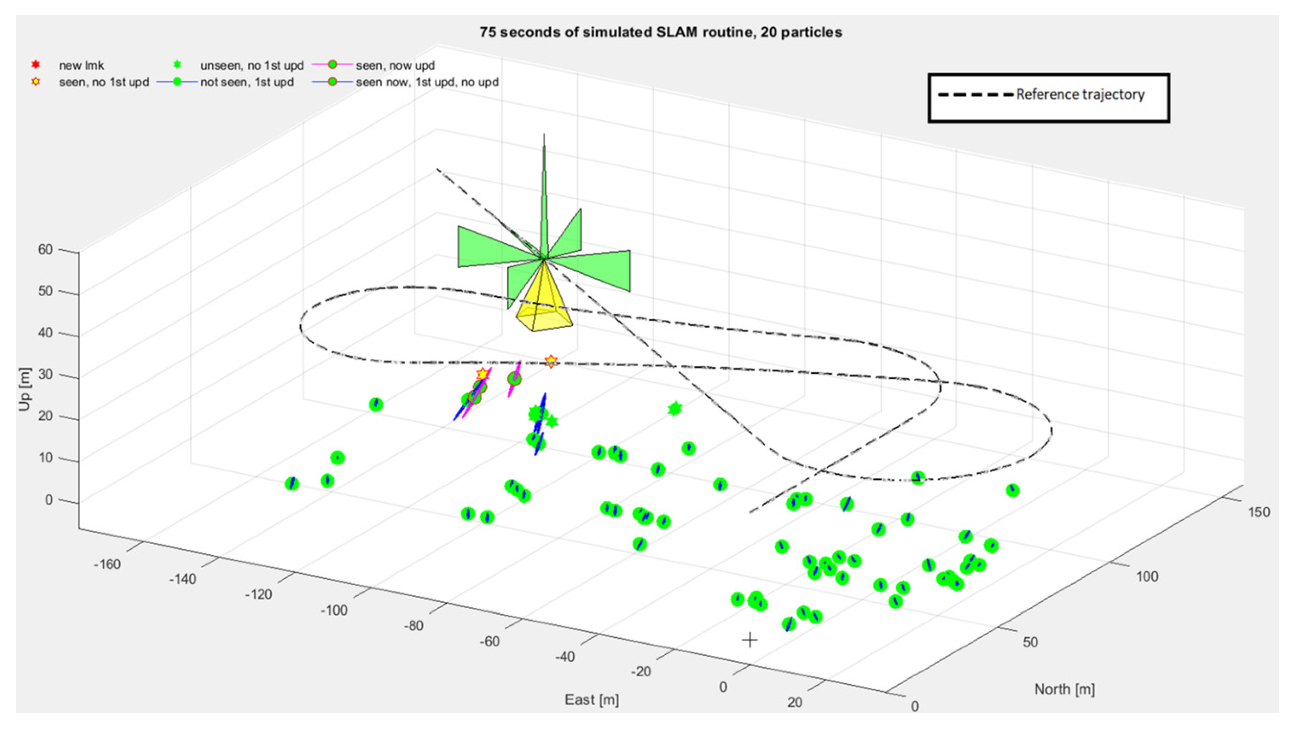
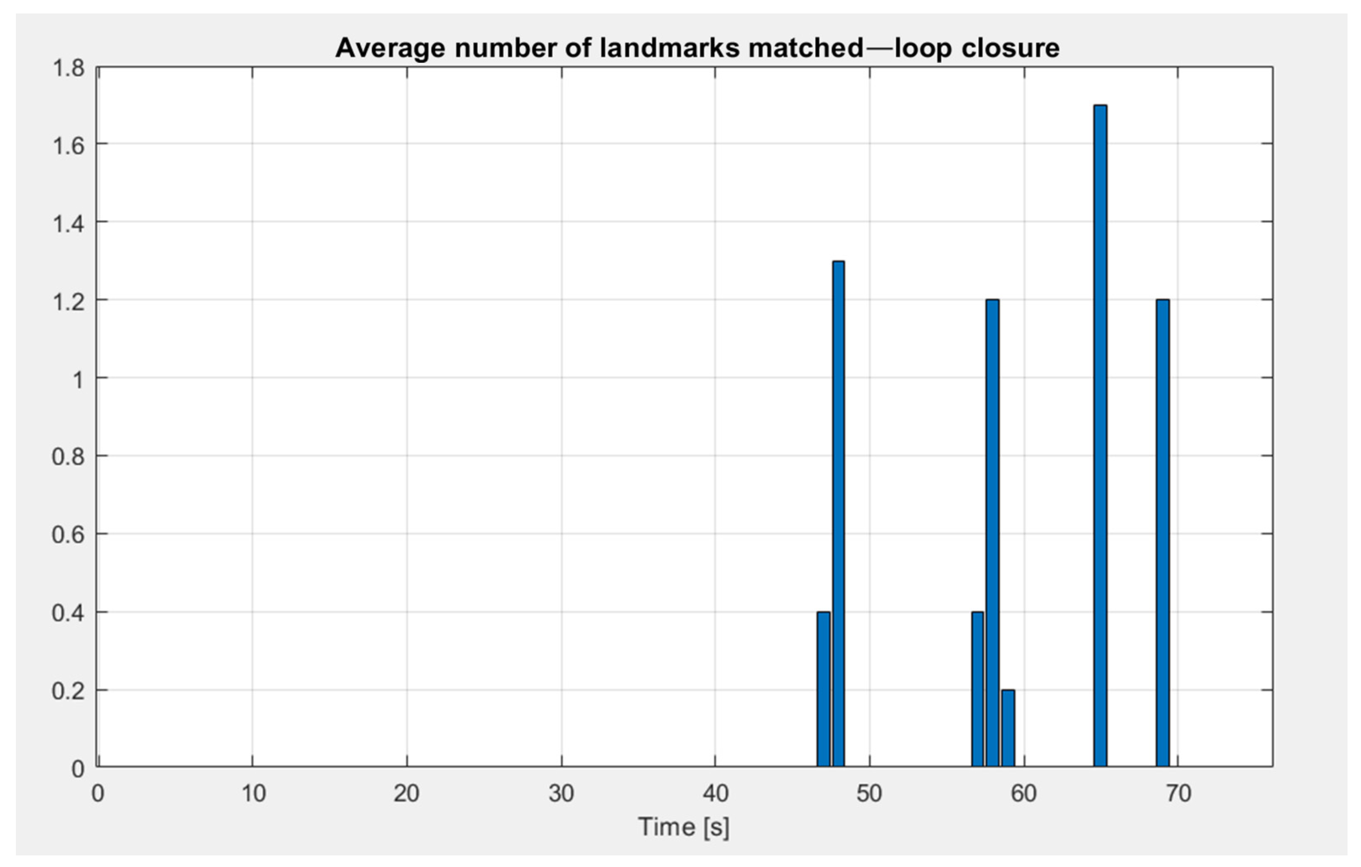
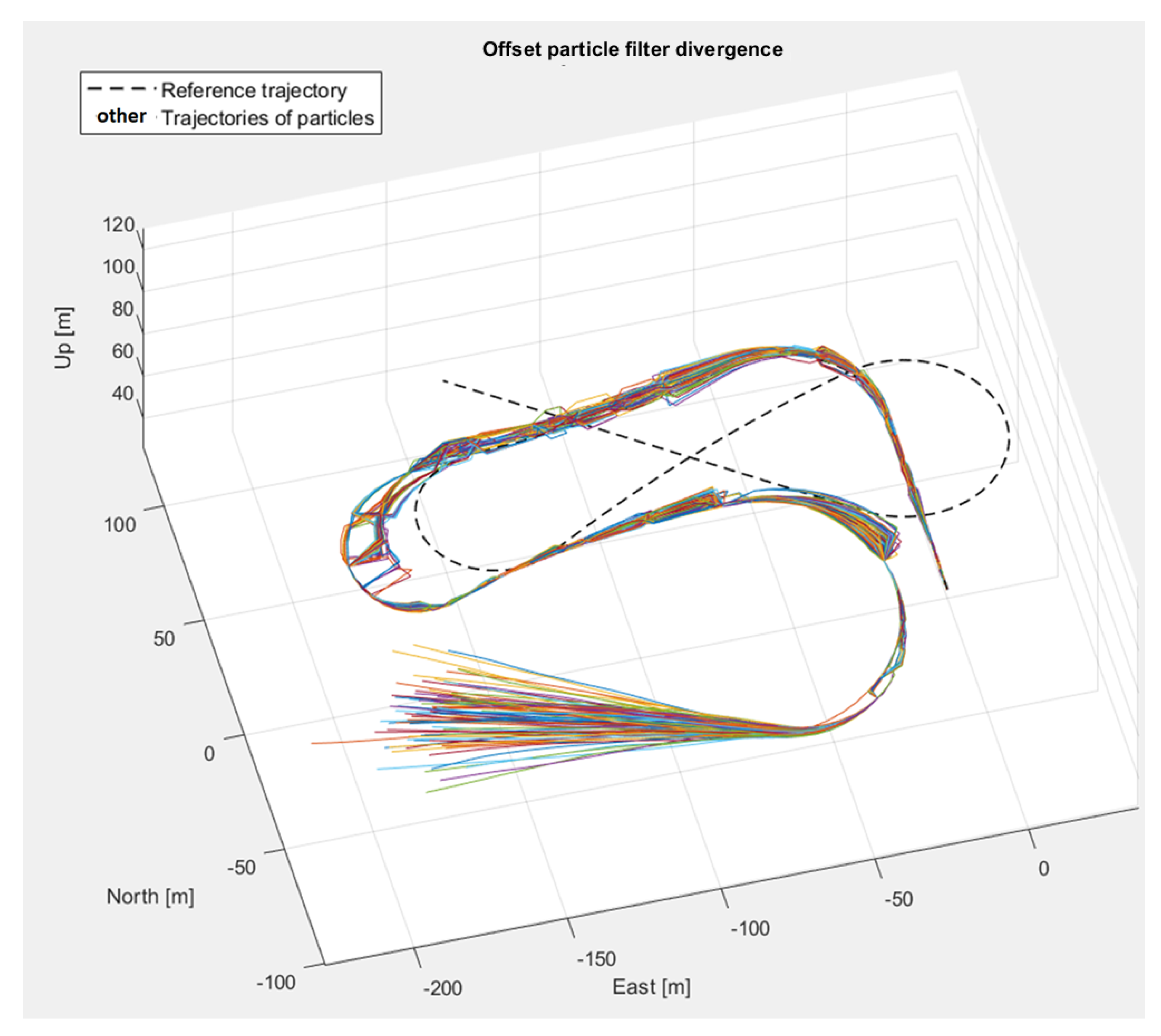
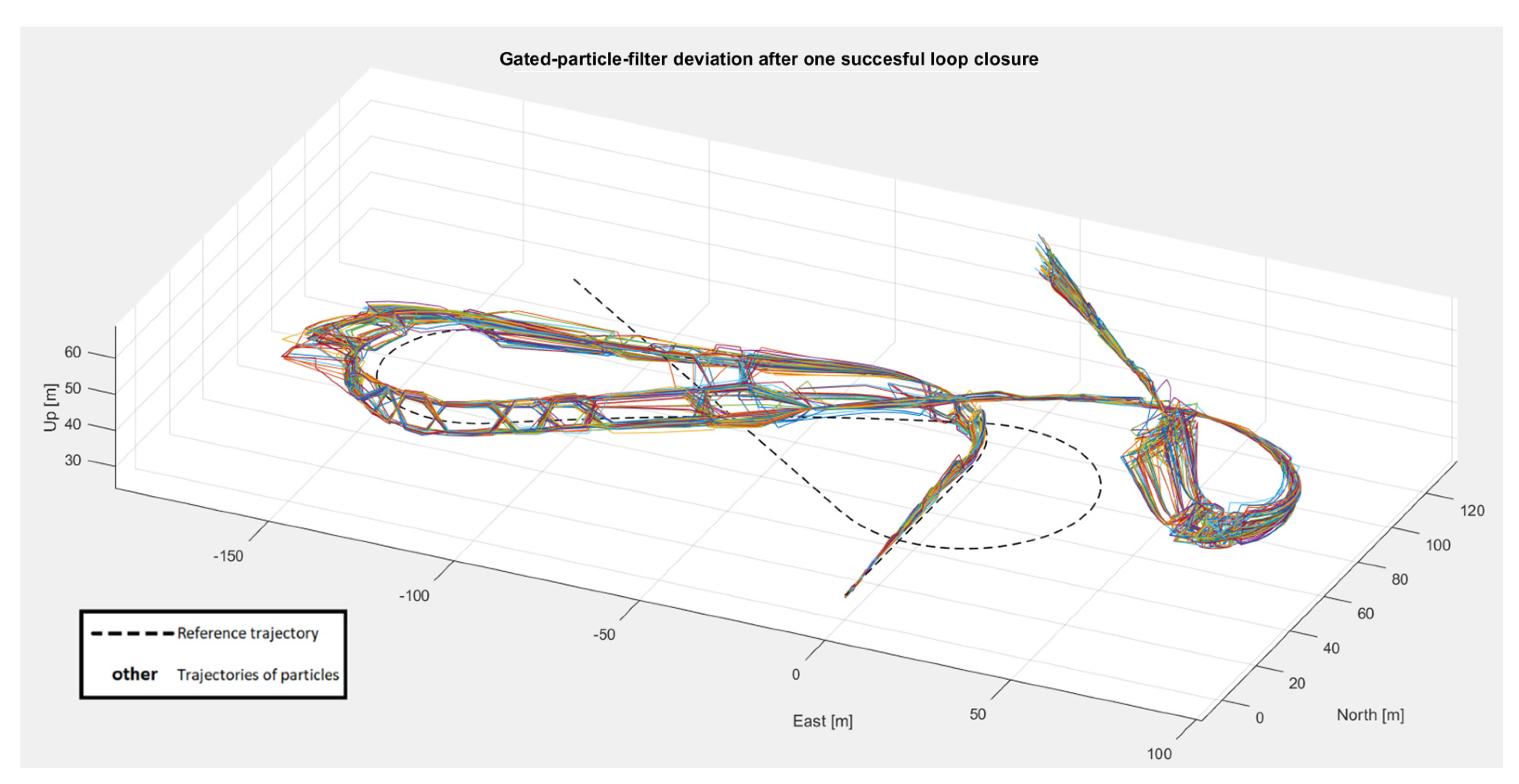
However, the significantly poorer performance of the last two methods led to their exclusion from the undertaken evaluation.

4.1. Simulation

Simulations were predominantly used to examine the overall cohesion of different solutions. First of all, this type of approach allowed the SLAM procedure to be performed in precisely defined conditions, e.g., exactly known UAV trajectory, camera orientation, sensor noise, etc. Availability of the reference trajectory is of particular value, as it enables the calculation of positioning errors.

The robotics simulator chosen to generate data for the evaluation of the performance of the compared methods was the Gazebo open-source software [47]. Gazebo was adopted, as it is the most-known robotic simulator, accepted as the de facto software platform for robotics [48,49,50]. The experiment configuration was built upon a set of two sensors following a predefined trajectory. The camera was pointed directly downwards and the IMU provided 3D accelerations and angular velocities. To achieve similarity between the real world and the simulation environment, we used an aerial photograph, taken from a UAV, and stretched it over the ground plane in Gazebo. The exemplary simulation setup is presented in Figure 8, where the sensor is marked with a red ellipse.

An exemplary map-building process (Figure 9) that emerged during one of our SLAM-algorithm runs is presented below. The landmarks are shown as either green circles (those scene points which were updated at least once) with a blue $1\sigma$ ellipsoid uncertainty region or as green stars (those scene points that were not yet updated). Ellipsoids in magenta denote landmarks being updated at the given time step. If the landmark is seen (correctly matched) in the currently processed frame, its edge is red, and if a landmark is newly observed, the marker is red.

We tested the listed approaches, using a scenario in which the UAV was flying at an altitude of 30 m. The trajectory of the drone was chosen in a way that created four areas in which there was a possibility for a loop closure. The flight took about 75 s, during which the vehicle traveled almost 900 m. An example of a SLAM procedure’s results, for simulations conducted using the above-discussed scenario, is presented in Figure 10, where the reference track is marked in black and all other colored lines represent the paths of single particles. The areas where a potential loop-closing procedure can be performed are marked with blue ellipses.

In the example above, the achieved root-mean-square (RMS) error of the trajectory, using only 20 particles, is less than 3.3 m.

To evaluate the performance of different approaches to gating and weighting procedures, we performed a set of simulation runs for each approach, after which we averaged the results. The data collected during the tests are presented in

Table 1. Comparison of simulation results.

Number of particles		20			40			80
Weighting and gating approach		1	2	3	1	2	3	1	2	3
Percent of correct loop closures	loop 4	90	0	20	80	10	30	90	30	30
	loop 3	90	0	20	80	10	30	100	60	30
	loop 2	100	0	30	100	10	30	100	60	40
	loop 1	100	0	50	100	20	60	100	80	70
Number of resamplings		62.11	-	37.5	68.5	29	50.33	68.22	63.67	53
Root mean squared error [m]		20.34	-	34.23	13.545	29.95	28.68	7.80	17.33	15.97

. The indexes of the weighting and gating approach match the order of the list in the first paragraph of this section.

The compared methods were analyzed in terms of overall accuracy—trajectory RMS error—as well as the ability to correctly close the loop. The loop closure was considered successful if there were landmark matches for scene points which had not been seen during the previous 5 s of observation. It was convenient to analyze this condition using a plot, an example of which can be seen in Figure 11, where all four successful loop closures are visible.

Moreover, the total number of resampling procedures which took place during the flight was compared. Every set of the filter settings was evaluated 10 times. However, only those runs which ended in the successful closing of all four loops are included in the mean calculations.

The overall filter performance, interpreted as the ability to follow a given path accurately and evaluated using the amount of correctly closed loops, points to our novel stratification method as the most reliable one. Even for as little as 20 particles, the algorithm using our approach was able to reach the end of the trajectory accurately enough to close the last loop almost every time. On the contrary, the approach, which limited weight adjustment only to the addition of penalties in accordance to Equation (24,) resulted in the inability to correctly follow the true trajectory, even once, when using 20 particles. The increase in the number of particles improved its effectiveness, but even the employment of 80 particles led to successful closures of all loops in only 30% of runs. Although the third approach performed slightly better than the previous one, it was still erroneous most of the time. Similar conclusions can be drawn when analyzing the RMS errors, as the novel stratification method proves to be significantly more accurate.

To present the manner in which different SLAM algorithms diverged from the reference trajectory, three examples are presented in Figure 12, Figure 13 and Figure 14.

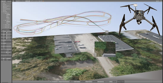
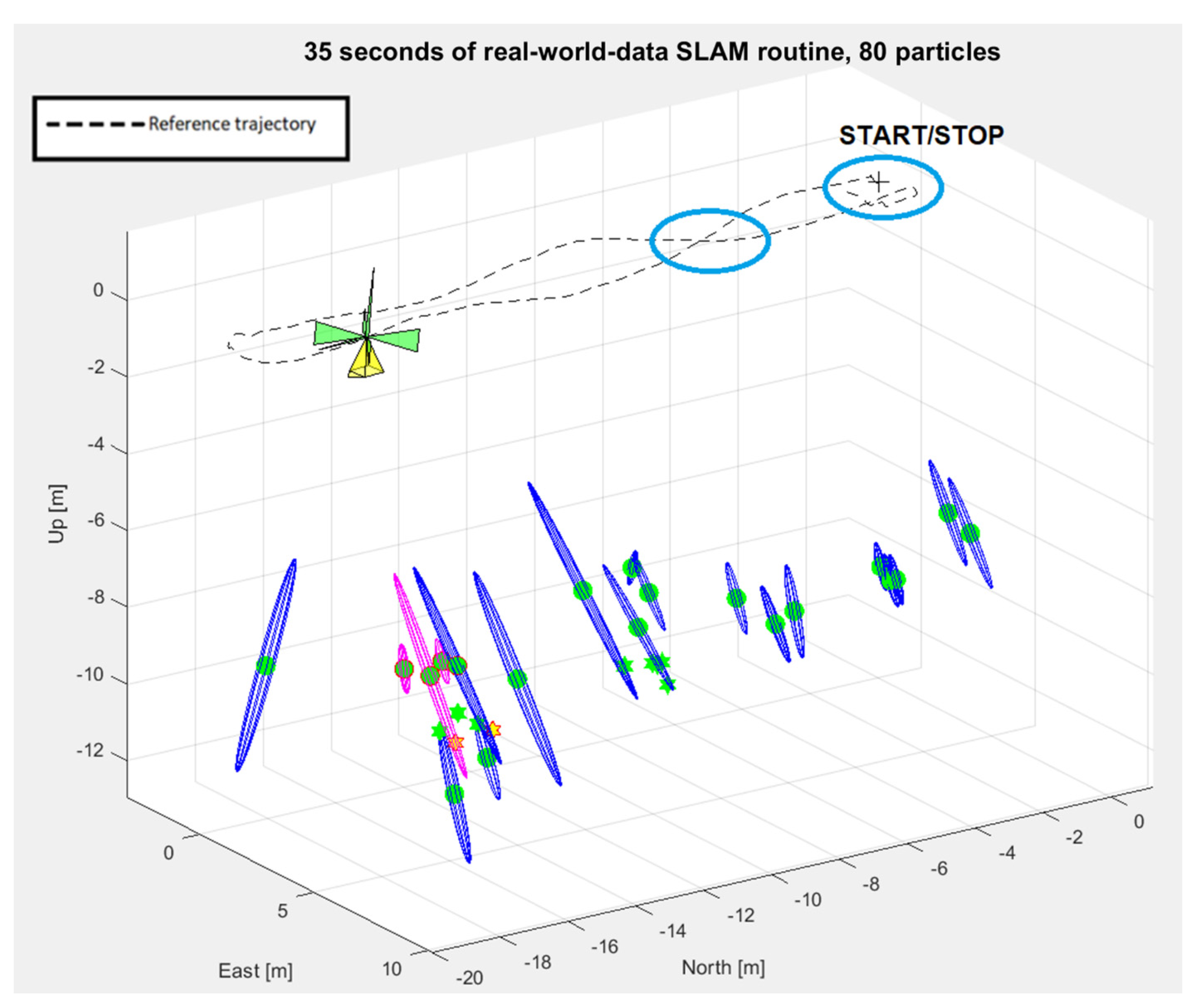
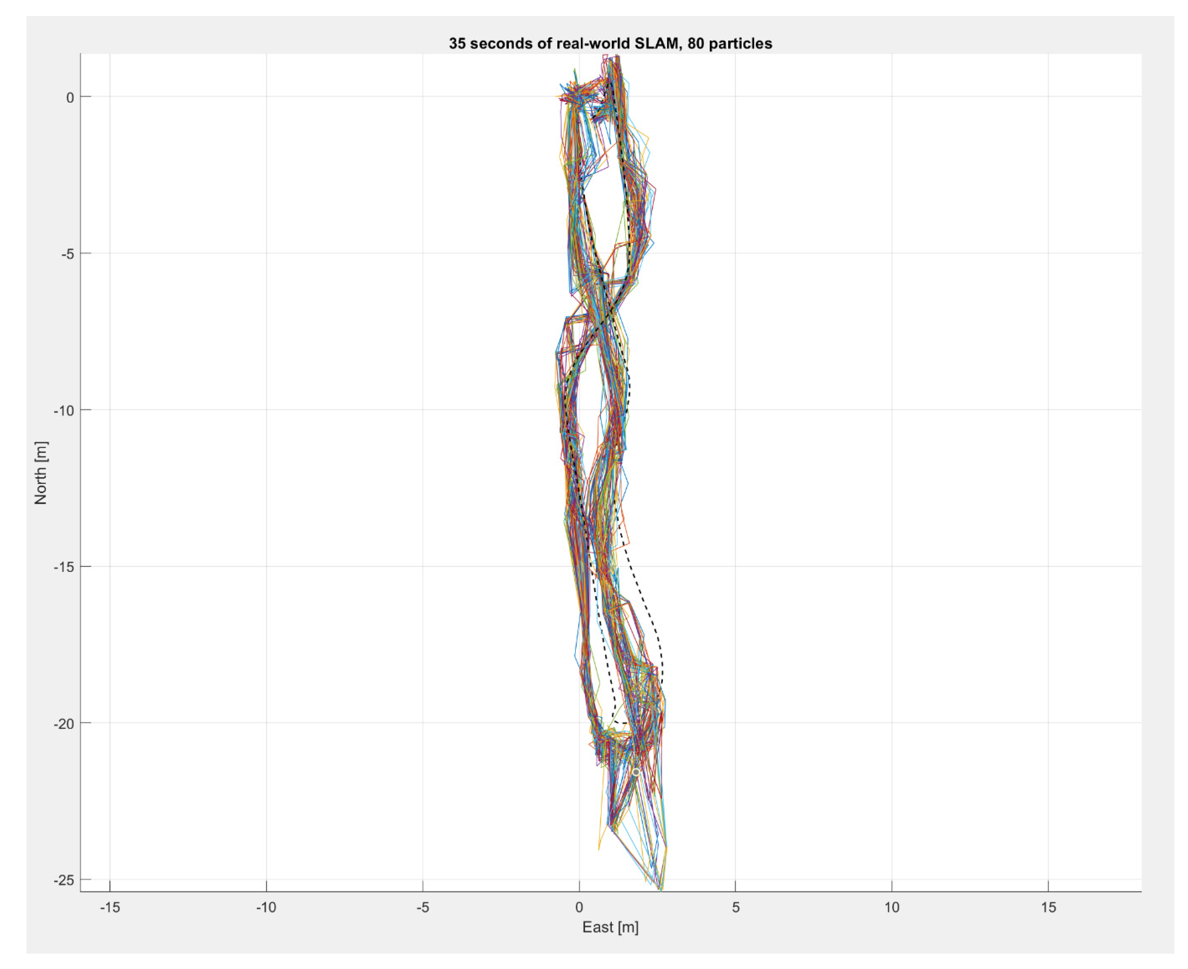
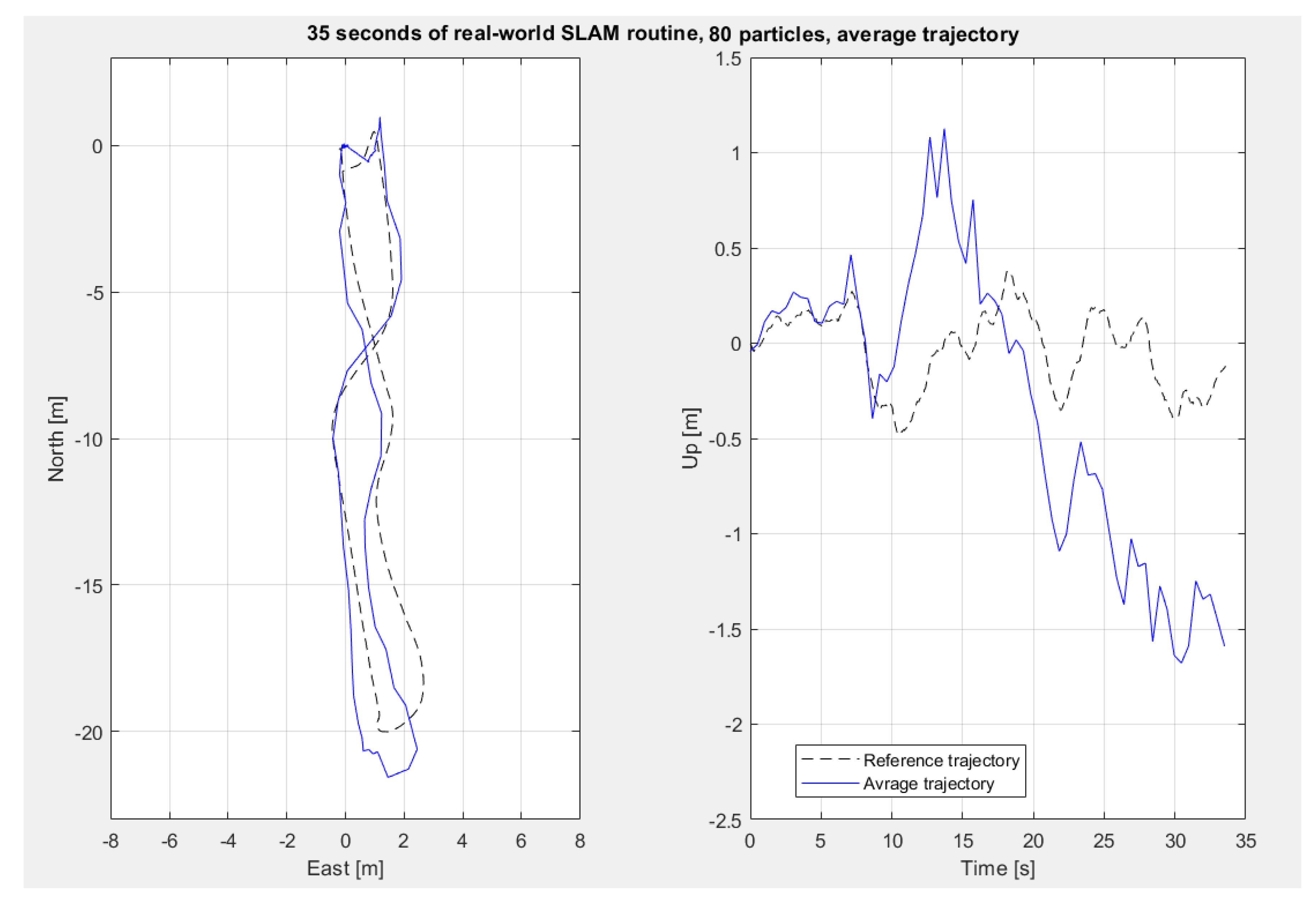
4.2. Real-World Data

To evaluate the utility of our approach more profoundly, we compared the SLAM procedures using real-world data from a UAV. The data were collected using the DJI Matrice M100, with a Raspberry Pi as an onboard computer—shown in Figure 15. Images were recorded using a Zenmuse X3 camera, while the onboard IMU was the source of kinematic data—one significantly less accurate than the sensor simulated in the previously described experiment.

The flight took place in the area where the aerial picture for the Gazebo simulation was taken. It lasted about 35 s, during which the UAV’s altitude varied between 10 and 13 m above ground.

The mapping concept is similar to the one for the simulation experiment, however, we assumed that the starting point of the UAV is point (0,0,0) in the local ENU coordinate frame. As the data were registered outdoors, no ground-truth trajectory was available. Hence, we compared the results of our SLAM algorithm to the data from an INS/GNSS integrated navigation system installed onboard the UAV. Such a trajectory can be used to detect significant errors (e.g., filter divergence), but the RMS trajectory error, calculated with respect to it, can be treated as a crude estimate of positioning error only.

First, to show the trajectory and the mapping procedure, we present the result of an exemplary SLAM procedure run in Figure 16. The areas of potential loop closure are marked with blue ellipses.

Below, the results of comparisons between the SLAM procedures are presented. The algorithm was examined using nine sets of parameters, analogously to the previous examination. However, only two potential loop closures are possible for the assumed flight trajectory. Moreover, the beginning and the end of the trajectory are localized very close in space. The data collected during the runs are presented in

Table 2. Comparison of real-world data processing results.

Number of particles		20			40			80
Weighting and gating approach		1	2	3	1	2	3	1	2	3
Percent of correct loop closures	loop 2	0	0	0	20	-	30	60	0	40
	loop 1	30	0	0	50	-	40	90	0	70
Number of resamplings		-	-	-	85.5	-	72.5	76.25	-	67.17
Root-mean-square error [m]		-	-	-	10.44	-	12.28	5.94	-	7.16

.

The most apparent conclusion is that the solution of the SLAM problem for this set of data proved to be significantly more difficult than for the simulated data. However, the results are similar, i.e. our stratified-filter approach performed more robustly and more accurately than the others. It was the only filter variant to correctly identify the turning-back maneuver—the first loop closure—using as few as 20 particles. Secondly, the performance of the approach with penalties for unmatched landmarks was least effective. We conducted an additional simulation to see whether this method would close at least the first loop correctly with 160 particles. Still, every run of the algorithm was unsuccessful.

In Figure 17, the trajectories of single particles, together GNSS reference trajectory, are shown, using horizontal projection for image clarity.

In Figure 18, the average track for this run is presented. The altitude is shown separately in the right subplot.

5. Discussion

The simulations and experiments compiled for compare different weighting and gating approaches for a PF SLAM provide consistent results that justify the implementation of the described stratification algorithm. First of all, its accuracy, measured in terms of RMSE, is superior. Secondly, the robustness of the algorithm is demonstrated by its having the highest percentage of successful runs. Last but not least, the amount of resampling procedures performed in different variants suggests that the method of data processing, in the stratified approach, provided the largest amount of information, as it led to more distinct differences in sample weights and more frequent resampling.

As mentioned earlier, the method of real-world data registration provided no ground-truth trajectory. This can be considered an additional source of uncertainty, in terms of accurate RMSE calculation, however, its impact should not be overestimated, because the INS/GNSS trajectory was available. Still, the removal of such an uncertainty can be pointed out as a future research direction, and we plan to implement our algorithm on a platform which will be capable of performing real-time kinematic (RTK) surveying. This will allow centimeter-level accuracy of positioning in providing reference trajectories.

6. Conclusions

This article discusses a particle-filter-SLAM algorithm that introduces a novel approach to the particle-weighting procedure.

Theoretical analysis and experimental evaluation were conducted for multiple simulated and real-world flights. As a result, the usage of Mahalanobis gating with weight stratification by the number of matched landmarks, was identified to be a beneficial and desirable element of monocular-particle-filter-SLAM algorithms.

The experiments proved that, overall, performance of a particle filter’s simultaneous localization-and-mapping algorithm is better when the presented approach is implemented. The stratified particle filter is more robust and accurate than other filter variants. Furthermore, the loop closure is performed more effectively and the particles are resampled more often.

Consequently, the application of the presented algorithm allows to reduce the number of particles—lowering the computational complexity.

References

1. Cadena, C.; Carlone, L.; Carrillo, H.; Latif, Y.; Scaramuzza, D.; Neira, J.; Reid, I.; Leonard, J.J. Past, present, and future of simultaneous localization and mapping: Toward the robust-perception age. IEEE Trans. Robot. 2016, 32, 1309–1332. [Google Scholar] [CrossRef] [Green Version]
2. Younes, G.; Asmar, D.; Shammas, E.; Zelek, J. Keyframe-based monocular SLAM: Design, survey, and future directions. Rob. Auton. Syst. 2017, 98, 67–88. [Google Scholar] [CrossRef] [Green Version]
3. Solà, J.; Vidal-Calleja, T.; Civera, J.; Montiel, J.M.M. Impact of landmark parametrization on monocular EKF-SLAM with points and lines. Int. J. Comput. Vis. 2012, 97, 339–368. [Google Scholar] [CrossRef]
4. Durrant-Whyte, H.; Bailey, T. Simultaneous localization and mapping: Part I. IEEE Robot. Autom. Mag. 2006, 13, 99–108. [Google Scholar] [CrossRef] [Green Version]
5. Wang, H.; Fu, G.; Li, J.; Yan, Z.; Bian, X. An Adaptive UKF Based SLAM Method for Unmanned Underwater Vehicle. Math. Probl. Eng. 2013, 2013, 605981. [Google Scholar] [CrossRef] [Green Version]
6. Montemerlo, M.; Thrun, S.; Koller, D.; Wegbreit, B. FastSLAM: A factored solution to the simultaneous localization and mapping problem. In Proceedings of the National Conference on Artificial Intelligence, Edmonton, AB, Canada, 28 July–1 August 2002; pp. 593–598. [Google Scholar]
7. Thrun, S.; Montemerlo, M.; Koller, D.; Wegbreit, B.; Nieto, J.; Nebot, E. Fastslam: An efficient solution to the simultaneous localization and mapping problem with unknown data association. J. Mach. Learn. Res. 2004, 4, 380–407. [Google Scholar]
8. Grisetti, G.; Kummerle, R.; Stachniss, C.; Burgard, W. A Tutorial on Graph-Based SLAM. IEEE Intell. Transp. Syst. Mag. 2010, 2, 31–43. [Google Scholar] [CrossRef]
9. Strasdat, H.; Montiel, J.M.M.; Davison, A.J. Real-time monocular SLAM: Why filter? In Proceedings of the IEEE International Conference on Robotics and Automation, Anchorage, AK, USA, 3–7 May 2010; pp. 2657–2664. [Google Scholar] [CrossRef] [Green Version]
10. Minkler, G.; Minkler, J. Theory and Application of Kalman Filtering; Magellan Book Co.: Palm Bay, FL, USA, 1993; ISBN 0962161829. [Google Scholar]
11. Mur-Artal, R.; Montiel, J.M.M.; Tardos, J.D. ORB-SLAM: A Versatile and Accurate Monocular SLAM System. IEEE Trans. Robot. 2015, 31, 1147–1163. [Google Scholar] [CrossRef] [Green Version]
12. Altermatt, M.; Martinelli, A.; Tomatis, N.; Siegwart, R. SLAM with comer features based on a relative map. In Proceedings of the 2004 IEEE/RSJ International Conference on Intelligent Robots and Systems (IROS) (IEEE Cat. No. 04CH37566), Sendai, Japan, 28 September–2 October 2004; Volume 2, pp. 1053–1058. [Google Scholar]
13. An, S.-Y.; Kang, J.-G.; Lee, L.-K.; Oh, S.-Y. SLAM with salient line feature extraction in indoor environments. In Proceedings of the 2010 11th International Conference on Control Automation Robotics & Vision, Singapore, 7–10 December 2010; pp. 410–416. [Google Scholar]
14. Pillai, S.; Leonard, J. Monocular SLAM Supported Object Recognition. In Proceedings of the Robotics: Science and Systems XI, Rome, Italy, 13–17 July 2015; Volume 11. [Google Scholar]
15. Eade, E.; Drummond, T. Scalable Monocular SLAM Simultaneous Localization and Mapping. In Proceedings of the IEEE Computer Society Conference on Computer Vision and Pattern Recognition, New York, NY, USA, 17–22 June 2006; pp. 469–476. [Google Scholar] [CrossRef]
16. Civera, J.; Lee, S.H. RGB-D Odometry and SLAM. In Advances in Computer Vision and Pattern Recognition; Springer: Berlin/Heidelberg, Germany, 2019; pp. 117–144. ISBN 9783030286033. [Google Scholar]
17. Bresson, G.; Alsayed, Z.; Yu, L.; Glaser, S. Simultaneous Localization and Mapping: A Survey of Current Trends in Autonomous Driving. IEEE Trans. Intell. Veh. 2017, 2, 194–220. [Google Scholar] [CrossRef] [Green Version]
18. Saeedi, S.; Trentini, M.; Li, H.; Seto, M. Multiple-robot Simultaneous Localization and Mapping-A Review 1 Introduction 2 Simultaneous Localization and Mapping: Problem statement. J. F. Robot. 2016, 33, 3–46. [Google Scholar] [CrossRef]
19. Kaniewski, P.; Słowak, P. Simulation and Analysis of Particle Filter Based Slam System. Annu. Navig. 2019, 25, 137–153. [Google Scholar] [CrossRef] [Green Version]
20. Murphy, K.P. Bayesian map learning in dynamic environments. In Advances in Neural Information Processing Systems; MIT Press: Cambridge, MA, USA, 2000; pp. 1015–1021. [Google Scholar]
21. Qian, K.; Ma, X.; Dai, X.; Fang, F. Improved Rao-Blackwellized particle filter for simultaneous robot localization and person-tracking with single mobile sensor. J. Control Theory Appl. 2011, 9, 472–478. [Google Scholar] [CrossRef]
22. Carlone, L.; Kaouk Ng, M.; Du, J.; Bona, B.; Indri, M. Simultaneous localization and mapping using rao-blackwellized particle filters in multi robot systems. J. Intell. Robot. Syst. Theory Appl. 2011, 63, 283–307. [Google Scholar] [CrossRef] [Green Version]
23. Xuexi, Z.; Guokun, L.; Genping, F.; Dongliang, X.; Shiliu, L. SLAM algorithm analysis of mobile robot based on lidar. In Proceedings of the 2019 Chinese Control Conference (CCC), Guangzhou, China, 27–30 July 2019; pp. 4739–4745. [Google Scholar] [CrossRef]
24. Kwok, N.M.; Dissanayake, G. Bearing-only SLAM in indoor environments using a modified particle filter. In Proceedings of the Australasian Conference on Robotics Automation 2003, Brisbane, Australia, 1–3 December 2003. [Google Scholar]
25. Pupilli, M.L.; Calway, A.D. Real-Time Camera Tracking Using a Particle Filter. In Proceedings of the British Machine Vision Conference, Oxford, UK, 5–8 September 2005; British Machine Vision Association: Durham, UK, 2005; pp. 519–528. [Google Scholar]
26. Sim, R.; Elinas, P.; Griffin, M.; Little, J.J. Vision-based SLAM using the rao-blackwellised particle filter. In Proceedings of the IJCAI-05 Workshop Reasoning with Uncertainty in Robotics (RUR-05), Edinburgh, UK, 30 July 2005; Volume 14, pp. 9–16. [Google Scholar]
27. Lowe, D.G. Object recognition from local scale-invariant features. In Proceedings of the IEEE International Conference on Computer Vision, Kerkyra, Greece, 20–27 September 1999; Volume 2, pp. 1150–1157. [Google Scholar]
28. Lemaire, T.; Lacroix, S.; Sola, J. A practical 3D bearing-only SLAM algorithm. In Proceedings of the 2005 IEEE/RSJ International Conference on Intelligent Robots and Systems, Edmonton, AB, Canada, 2–6 August 2005; pp. 2449–2454. [Google Scholar]
29. Strasdat, H.; Stachniss, C.; Bennewitz, M.; Burgard, W. Visual Bearing-Only Simultaneous Localization and Mapping with Improved Feature Matching. In Proceedings of the Autonome Mobile Systeme 2007, 20. Fachgespräch, Kaiserslautern, Germany, 18–19 October 2007; pp. 15–21. [Google Scholar]
30. Bay, H.; Ess, A.; Tuytelaars, T.; Van Gool, L. Speeded-Up Robust Features (SURF). Comput. Vis. Image Underst. 2008, 110, 346–359. [Google Scholar] [CrossRef]
31. Kwon, J.; Lee, K.M. Monocular SLAM with locally planar landmarks via geometric rao-blackwellized particle filtering on Lie groups. In Proceedings of the 2010 IEEE Computer Society Conference on Computer Vision and Pattern Recognition, San Francisco, CA, USA, 13–18 June 2010; pp. 1522–1529. [Google Scholar]
32. Lee, S.-H. Real-time camera tracking using a particle filter combined with unscented Kalman filters. J. Electron. Imaging 2014, 23, 013029. [Google Scholar] [CrossRef]
33. Ababsa, F.; Mallem, M. Robust camera pose tracking for augmented reality using particle filtering framework. Mach. Vis. Appl. 2011, 22, 181–195. [Google Scholar] [CrossRef]
34. Harris, C.; Stephens, M. A Combined Corner and Edge Detector. In Proceedings of the Alvey Vision Conference, Manchester, UK, 31 August–2 September 1988; pp. 147–151. [Google Scholar]
35. Çelik, K.; Somani, A.K. Monocular Vision SLAM for Indoor Aerial Vehicles. J. Electr. Comput. Eng. 2013, 2013, 374165. [Google Scholar] [CrossRef] [Green Version]
36. Vidal, F.S.; Barcelos, A.D.O.P.; Rosa, P.F.F. SLAM solution based on particle filter with outliers filtering in dynamic environments. In Proceedings of the IEEE 24th International Symposium on Industrial Electronics (ISIE), Buzios, Brazil, 3–5 June 2015; pp. 644–649. [Google Scholar] [CrossRef]
37. Hoseini, S.; Kabiri, P. A Novel Feature-Based Approach for Indoor Monocular SLAM. Electronics 2018, 7, 305. [Google Scholar] [CrossRef] [Green Version]
38. Zhou, Y.; Maskell, S. RB2-PF: A novel filter-based monocular visual odometry algorithm. In Proceedings of the 2017 20th International Conference on Information Fusion (Fusion), Xi’an, China, 10–13 July 2017. [Google Scholar] [CrossRef]
39. Chen, X.; Zhang, H.; Lu, H.; Xiao, J.; Qiu, Q.; Li, Y. Robust SLAM system based on monocular vision and LiDAR for robotic urban search and rescue. In Proceedings of the 2017 IEEE International Symposium on Safety, Security and Rescue Robotics (SSRR), Shanghai, China, 11–13 October 2017; pp. 41–47. [Google Scholar] [CrossRef]
40. Wang, S.; Kobayashi, Y.; Ravankar, A.A.; Ravankar, A.; Emaru, T. A Novel Approach for Lidar-Based Robot Localization in a Scale-Drifted Map Constructed Using Monocular SLAM. Sensors 2019, 19, 2230. [Google Scholar] [CrossRef] [Green Version]
41. Acevedo, J.J.; Messias, J.; Capitan, J.; Ventura, R.; Merino, L.; Lima, P.U. A Dynamic Weighted Area Assignment Based on a Particle Filter for Active Cooperative Perception. IEEE Robot. Autom. Lett. 2020, 5, 736–743. [Google Scholar] [CrossRef]
42. Deng, X.; Mousavian, A.; Xiang, Y.; Xia, F.; Bretl, T.; Fox, D. PoseRBPF: A Rao–Blackwellized Particle Filter for 6-D Object Pose Tracking. IEEE Trans. Robot. 2021. [Google Scholar] [CrossRef]
43. Yuan, D.; Lu, X.; Li, D.; Liang, Y.; Zhang, X. Particle filter re-detection for visual tracking via correlation filters. Multimed. Tools Appl. 2019, 78, 14277–14301. [Google Scholar] [CrossRef] [Green Version]
44. Zhang, Q.; Wang, P.; Chen, Z. An improved particle filter for mobile robot localization based on particle swarm optimization. Expert Syst. Appl. 2019, 135, 181–193. [Google Scholar] [CrossRef]
45. Montiel, J.M.M.; Civera, J.; Davison, A.J. Unified inverse depth parametrization for monocular SLAM. Robot. Sci. Syst. 2007, 2, 81–88. [Google Scholar] [CrossRef]
46. Tareen, S.A.K.; Saleem, Z. A comparative analysis of SIFT, SURF, KAZE, AKAZE, ORB, and BRISK. In Proceedings of the 2018 International Conference on Computing, Mathematics and Engineering Technologies (iCoMET), Sukkur, Pakistan, 3–4 March 2018; pp. 1–10. [Google Scholar] [CrossRef]
47. Koenig, N.; Howard, A. Design and use paradigms for gazebo, an open-source multi-robot simulator. In Proceedings of the 2004 IEEE/RSJ International Conference on Intelligent Robots and Systems (IROS) (IEEE Cat. No.04CH37566), Sendai, Japan, 28 September–2 October 2004; Volume 3, pp. 2149–2154. [Google Scholar]
48. Ivaldi, S.; Peters, J.; Padois, V.; Nori, F. Tools for simulating humanoid robot dynamics: A survey based on user feedback. In Proceedings of the 2014 IEEE-RAS International Conference on Humanoid Robots, Madrid, Spain, 18–20 November 2014; pp. 842–849. [Google Scholar]
49. Gong, Z.; Liang, P.; Feng, L.; Cai, T.; Xu, W. Comparative Analysis Between Gazebo and V-REP Robotic Simulators. In Proceedings of the ICMREE 2011 International Conference on Materials for Renewable Energy and Environment, Shanghai, China, 20–22 May 2011; Volume 2, pp. 1678–1683. [Google Scholar] [CrossRef]
50. Körber, M.; Lange, J.; Rediske, S.; Steinmann, S.; Glück, R. Comparing Popular Simulation Environments in the Scope of Robotics and Reinforcement Learning. arXiv 2021, arXiv:2103.04616. [Google Scholar]
Figure 1. Frame from a downward-looking camera with extracted SURF features.
Remotesensing 13 03233 g001
Figure 2. IDP landmark parametrization.
Remotesensing 13 03233 g002
Figure 3. An example of bimodal PDF encoded using weighted particles.
Remotesensing 13 03233 g003
Figure 4. The flowchart of the weights stratification algorithm.
Remotesensing 13 03233 g004
Figure 5. Weights before stratification.
Remotesensing 13 03233 g005
Figure 6. Weights after stratification.
Remotesensing 13 03233 g006
Figure 7. The flowchart of the landmark removal procedure.
Remotesensing 13 03233 g007
Figure 8. Simulation environment.
Remotesensing 13 03233 g008
Figure 9. An exemplary map building process.
Remotesensing 13 03233 g009
Figure 10. Simulated SLAM routine for 20 particles.
Remotesensing 13 03233 g010
Figure 11. The average number of landmarks which were consequently matched after more than 5 s for the correct closure of all four loops.
Remotesensing 13 03233 g011
Figure 12. The example of filter divergence (method with adding penalty for unmatched landmarks).
Remotesensing 13 03233 g012
Figure 13. The example of filter divergence (method with weighting particles using only the lowest number of matched landmarks).
Remotesensing 13 03233 g013
Figure 14. The example of filter divergence (method without gating for the outliers removal).
Remotesensing 13 03233 g014
Figure 15. DJI Matrice 100 with an on-board computer.
Remotesensing 13 03233 g015
Figure 16. An exemplary map building procedure for real-world data.
Remotesensing 13 03233 g016
Figure 17. Real-world-data-SLAM routine for 80 particles.
Remotesensing 13 03233 g017
Figure 18. Average trajectory for the real-world-data-SLAM routine for 80 particles.
Remotesensing 13 03233 g018