Using Field Spectroradiometer to Estimate the Leaf N/P Ratio of Mixed Forest in a Karst Area of Southern China: A Combined Model to Overcome Overfitting

Abstract

The ratio between nitrogen and phosphorus (N/P) in plant leaves has been widely used to assess the availability of nutrients. However, it is challenging to rapidly and accurately estimate the leaf N/P ratio, especially for mixed forest. In this study, we collected 301 samples from nine typical karst areas in Guangxi Province during the growing season of 2018 to 2020. We then utilized five models (partial least squares regression (PLSR), backpropagation neural network (BPNN), general regression neural network (GRNN), PLSR+BPNN, and PLSR+GRNN) to estimate the leaf N/P ratio of plants based on these samples. We also applied the fractional differentiation to extract additional information from the original spectra of each sample. The results showed that the average leaf N/P ratio of plants was 17.97. Plant growth was primarily limited by phosphorus in these karst areas. The sensitive spectra to estimate leaf N/P ratio had wavelengths ranging from 400–730 nm. The prediction capabilities of these five models can be ranked in descending order as PLSR+GRNN, PLSR+BPNN, PLSR, GRNN, and BPNN when considering both accuracy and robustness. The PLSR+GRNN model yielded high R² and performance to deviation (RPD), and low root mean squared error (RMSE) with values of 0.91, 3.15, and 1.98, respectively, for the training test and 0.81, 2.25, and 2.46, respectively, for validation test. Compared with the PLSR model, both PLSR+BPNN and PLSR+GRNN models had higher accuracy and were more stable. Moreover, both PLSR+BPNN and PLSR+GRNN models overcame the issue of overfitting, which occurs when a single model is used to predict leaf N/P ratio. Therefore, both PLSR+BPNN and PLSR+GRNN models can be used to predict the leaf N/P ratio of plants in karst areas. Fractional differentiation is a promising spectral preprocessing technique that can improve the accuracy of models. We conclude that the leaf N/P ratio of mixed forest can be effectively estimated using combined models based on field spectroradiometer data in karst areas.

1. Introduction

Nitrogen (N) and phosphorus (P) are crucial functional elements for organisms [1] and play a vital role in plant physiological processes [2,3,4]. Changes of the N and P concentration are essential for the growth of plants, as they are closely related to photosynthesis, respiration, N₂ fixation, and organic matter mineralization [5]. N and P are the primary limiting nutrients for plant growth in most natural systems. An N/P ratio greater than 16 indicates that plant growth is limited by P, while an N/P ratio of less than 14 is limited by N. Values between 14 and 16 suggest either N or P can be limited, or plant growth is co-limited by both N and P [6,7], although there is no general consensus about an N/P ratio which is not limiting in either or both nutrients. Therefore, exploring the N and P stoichiometry of leaves plays a critical role in better understanding the survival and adaptation strategies of plants. However, current methods for monitoring N and P content mainly rely on laboratory analysis. The precision of these traditional analytical methods is high, but they are time-consuming, complex, and require difficult storage and transportation logistics of field samples, which limits rapid on-site and non-destructive detection [8]. As a real-time, fast, and non-destructive technology, spectral technology plays an increasingly important role in detecting nutrient acquisition and growth of plants.

The mechanism and methods of estimating leaf biochemical parameters with remote sensing techniques have been advanced in recent years, especially ground-based hyperspectral remote sensing. For example, Sonobe and Wang [9] used hyperspectral techniques to estimate the chlorophyll content in leaves of a deciduous forest, and found that the normalized difference spectral index using the first-order differentiation of reflectance at 522 and 728 nm was the best index. Zhao et al. [10] used a hyperspectral stepwise regression analysis to estimate the water content of apple tree canopies and found that an equidistant sampling method improved the prediction accuracy. Yamashita et al. found that machine learning methods can predict chlorophyll and N content based on field spectroradiometer [11]. However, most previous research has focused on estimating chlorophyll, water, organic carbon (C), and N. Few studies have investigated N/P and other stoichiometric ratios that are significant indicators of plant growth. The patterns found for N and P cannot be directly applied to N/P. For example, Cui et al. [8] proposed that N and P display a strong positive correlation with the spectral reflectance at 650 nm, while the N/P ratio displays a strong negative correlation with the spectral reflectance at 650 nm. Therefore, further studies of stoichiometric ratio estimation using field spectroradiometer are needed.

Previous studies on the spectral inversion of biochemical parameters focused on single species, such as rice [12], wheat [13], tobacco [14], apple [10], and tea [15]. As many species co-exist within natural habitats, results derived for single species or cropland is not applicable to investigate patterns in complex mixed forests. Therefore, establishing a database with multiple plants is critical to estimate plant biochemical parameters through remote sensing methods. However, mixed species samples are usually more difficult to collect, and it is more complex to predict biochemical parameters. In contrast, single plant species are easier to predict with high accuracy. For example, the best coefficient of determination (R²) for the estimation of leaf mass per area (LMA) in mixed-species by Cheng et al. [16] was 0.74, while Inoue et al. [17] produced an R² above 0.9 in rice. Further research is required to improve model accuracy to estimate biochemical parameters in mixed-species ecosystems.

In terms of the algorithm employed in previous studies, mainstream empirical methods can be summarized into three categories; spectral index methods [9], linear regression methods [13], and machine learning methods [11]. Both the spectral index and the linear regression methods focus on finding the linear relationship between spectral reflectance and plant biochemical parameters. By contrast, machine learning methods can calculate nonlinear relationships between spectral reflectance and plant biochemical parameters. Each method has limitations and advantages. Linear models use simple principles, are computationally efficient, and more robust in prediction accuracy, but are often inferior to machine learning methods in terms of prediction capability. Theoretically, there will be both linear and nonlinear relationships between spectral reflectance and biochemical parameters of plant leaves. Therefore, the use of a combined model including both linear and nonlinear methods may improve prediction capability.

Overfitting is a common problem in many empirical models, especially for machine learning methods [18], and can cause deceptive diagnostic results and reduce the transferability of the model. A small number of samples, a large number of variables, and high-dimensionality may lead to overfitting of the model [19]. Field spectroradiometer data are characterized by high-dimensionality and a large number of bands (variables), meaning that overfitting is a critical issue that has to be considered in the estimation of biochemical parameters. It has been proven that increasing data samples, cross-validation [20], regularization [19], noise removal [21], and integration of multiple models [22] are effective ways to overcome overfitting [23,24]. Therefore, combining linear and nonlinear models may be a way to reduce overfitting.

Spectral differentiation transform methods play an essential role in estimating plant parameters, and the most commonly used are spectral first-order and second-order differentiation [25]. It has been demonstrated that differential transformation of spectra can improve model performance for estimating plant water [10], chlorophyll [9], and N content [17,26]. However, the application of integer-order differentiation is not always sufficient, as the spectral curve shifts in shape from n-order to n + 1-order in a sharply fluctuating way, and there is no smooth transition between the intermediate stages. Fractional order transform methods allow differentiation from zero to arbitrary real numbers [27]. Using fractional order differentiation transforms spectra more continuously and produces more detailed information about the spectra.

The prediction of leaf N/P ratio of a particular species by field spectroradiometer has been reported [8,28], but directly estimating the leaf N/P ratio of all plants worldwide is difficult to achieve with current methods. Therefore, improving model performance and applying these methods to estimate leaf N/P ratio of regional mixed-species ecosystems is a pressing issue. Karst landscapes are one of the most crucial landform types globally, accounting for roughly 15% of the Earth’s total land area and inhabited by about 1 billion people [29]. Southwestern China has the largest karst area on the planet [30] and is one of 25 global biodiversity hotspots that contain many endemic and threatened species [31]. The karst areas of Guangxi Province are an important part of the southwest karst region, containing diverse landscape types, a wide variety of plants, and representing a key area for biodiversity conservation. However, anthropogenic disturbances have led to species loss in karst areas [32]. Non-destructive and rapid estimation of leaf N/P ratio of plants is required for ecological restoration and conservation in karst areas.

In this paper, we simulated the leaf N/P ratio of mixed forest in karst areas of Guangxi Province using fractional spectral differentiation and multiple models, combined with field spectroradiometer data. The primary objectives of this study are to (1) explore the predictive capabilities of linear regression models (partial least squares regression, PLSR) and nonlinear regression models (backpropagation neural network (BPNN), generalized neural network (GRNN)) to estimate leaf N/P ratio of mixed species based on field spectroradiometer data, (2) evaluate the contribution of fractional differentiation in improving these linear and nonlinear regression models’ performance, and (3) propose the best models that can overcome the insufficient accuracy of the PLSR model and overfitting of the BPNN and GRNN models to estimate leaf N/P ratio of plants in karst areas.

2. Materials and Methods

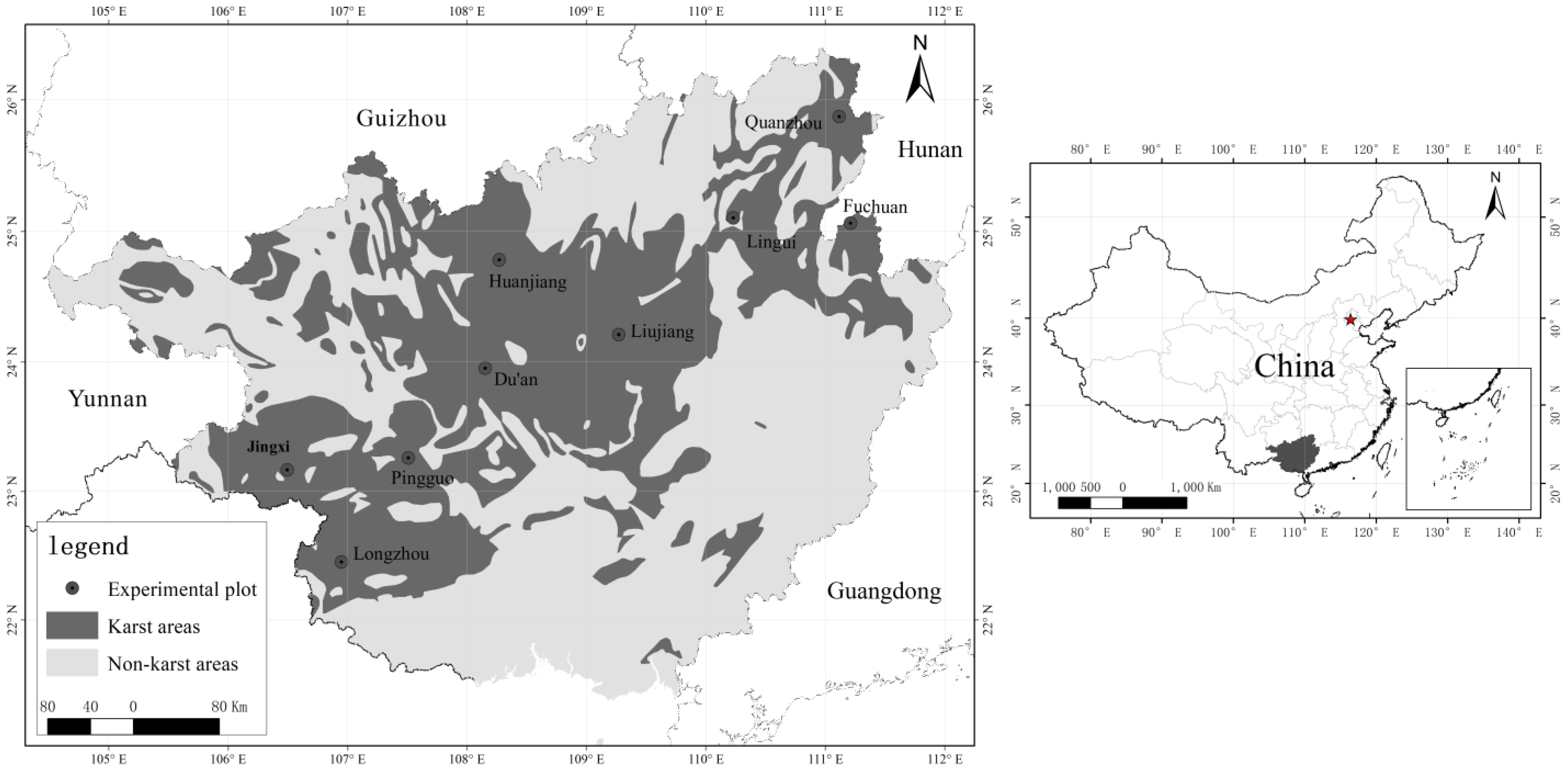
2.1. Study Area

The study area is located in Guangxi Province (20°54′–26°24′N, 104°28′–112°04′E) in south China (Figure 1). The elevation of the study area ranges from 0 to 2141.50 m. This area borders the South China Sea and has a tropical and subtropical climate. The average annual temperature ranges from 17.30 to 23.80 °C, and annual precipitation ranges from 1024.60 to 2358.60 mm. Karst landforms are distributed widely throughout Guangxi and cover about 97,000 km², accounting for 41% of the total area of the province. There are more than 4000 species of vascular plants, including more than 2000 species of medicinal plants, in the karst areas of Guangxi Province [33]. Nine typical karst experimental plots were selected, containing primary forests, secondary forests, and shrubs that represent the vegetation succession in karst areas. The area of each plot was about 200 m². Detailed information on each plot is described in

Table 1. Brief description of the experimental plots.

No.	Name of the Experimental Plot	Successional Stages of the Plant Community	Name of Dominant Species	Average Annual Temperature	Average Annual Rainfall
1	Jingxi	Secondary forest	Cladrastis platycarpa (Maxim.) Makino, Bruguiera gymnorhiza (L.) Lam., Buddleja officinalis, Abelia biflora Turcz.	21.68	1621.92
2	Longzhou	Primary forest	Canthium dicoccum, Memecylon scutellatum, Pistacia weinmanniifolia, Boniodendron minus, Excentrodendron hsienmu	23.28	1272.72
3	Pingguo	Shrubs	Rhus chinensis Mill., Cipadessa baccifera (Roth.) Miq., Vitex negundo L., Alchornea trewioides	22.03	1328.63
4	Du’an	Shrubs	Psidium guajava, Vitis heyneana, Buddleja officinalis, Serissa japonica	22.03	1733.37
5	Huanjiang	Secondary forest	Solanum indicum L., Ficus tinctoria Forst. F. subsp. gibbosa (Bl.) Corner, Albizia lebbeck (Linn.) Benth., Vitex negundo L.	22.50	1392.50
6	Liujiang	Secondary forest	Alchornea trewioides, Litsea glutinosa, Maclura cochinchinensis, Vitex negundo L.	21.57	1433.62
7	Lingui	Scrubs	Bauhinia championii, Zanthoxylum bungeanum, Sageretia thea, Rosa cymosa	21.56	1891.94
8	Quanzhou	Scrubs	Paliurus ramosissimus, Ilex corallina var. loeseneri, Bauhinia championii, Sageretia thea	21.65	1529.96
9	Fuchuan	Secondary forest	Albizia kalkora, Pistacia chinensis Bunge, Sapium sebiferum (L.) Roxb., Vitex negundo L.	19.47	1685.97

.

2.2. Data Collection

The leaves were sampled from July 2018 to September 2020. In each experimental plot, leaf samples from 8–15 plants of locally dominant species were collected. In total, the database includes 301 samples covering 37 families, 59 genera, and 70 species. As plants are susceptible to light conditions [34], we collected leaves from three directions for each plant (0–120°, 120–240°, and 240–360°, with 0° due north) to reduce random errors in samples.

Leaf spectral reflectance was measured in attached leaves using a spectroradiometer (Fieldspec 4, Analytical Spectral Devices, ASD, Boulder, CO, USA), with a spectral resolution of 3 nm in the visible and near-infrared (NIR) (350–1000 nm) and 8 nm in shortwave-infrared (SWIR, 1000–2500 nm) [14]. Reference plate (white reference) calibration was performed every 10 min during the measurement. Three branches of each tree were selected for measurement. As the instrument battery only has a continuous operating time of about 4 h in the field, only two mature and healthy leaves per branch were taken for spectral scanning due to time limitations. Finally, the scanned spectral reflectance of all leaves on each branch were arithmetically averaged, and the average value was taken as the spectral sample of each tree.

After the spectral measurements, the healthy and mature leaves on the branches were collected. It was then kept intact in a self-sealing bag and immediately placed in an incubator (ICERSICE940). Leaf samples were transported back to the laboratory within 24 h and dried at 75 °C. The dry samples were entirely sieved through a 100 mesh sieve for physicochemical analysis. Finally, the total nitrogen (TN) content of plant leaves was measured using the Kjeldahl method [35], and the total phosphorus (TP) content of plant leaves was measured by the phosphomolybdate blue spectrophotometry method [36]. The ratio of TN to TP was determined as the leaf N/P ratio.

2.3. Methodology

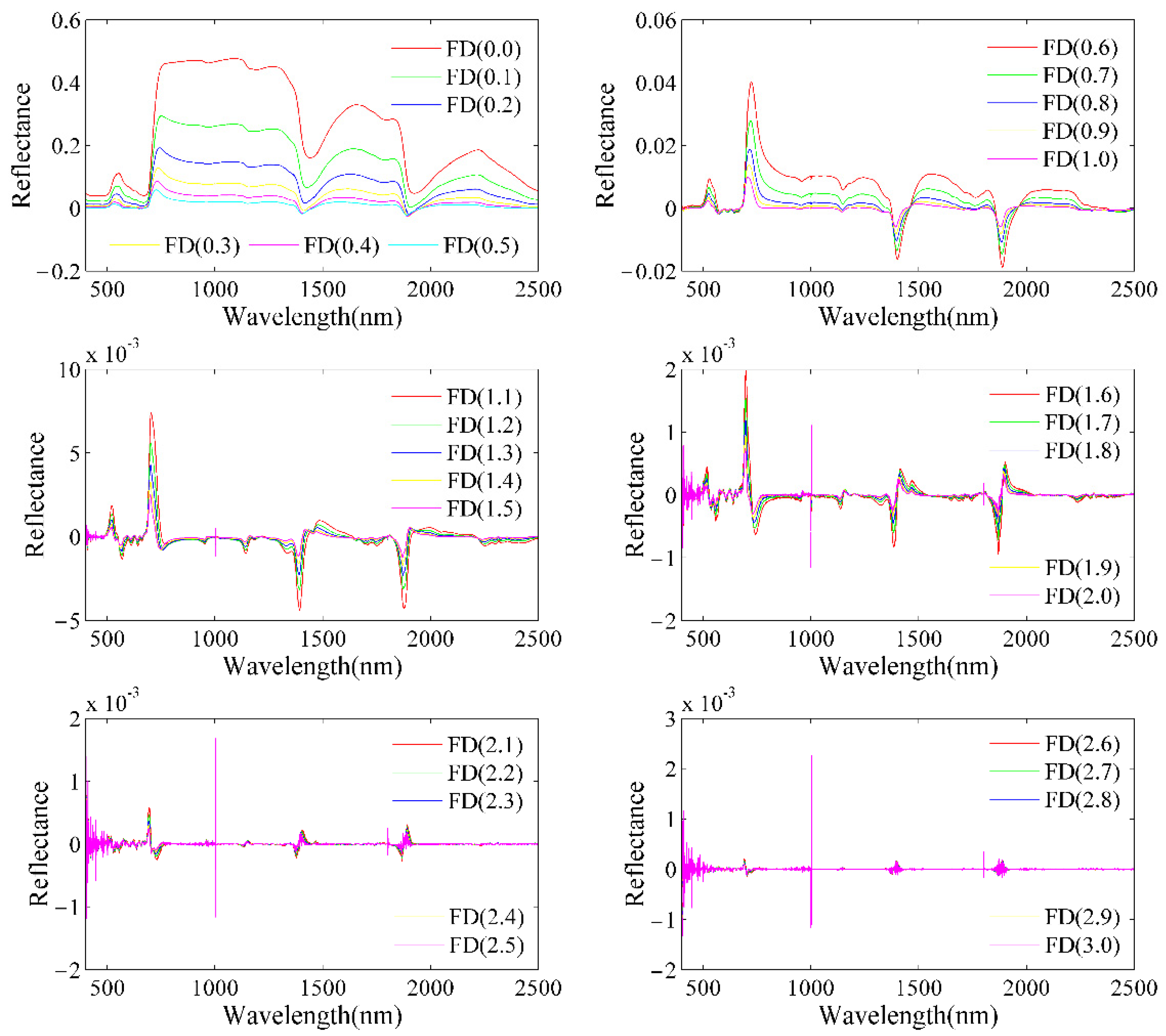
2.3.1. Fractional Differentiation (FD)

Fractional differentiation is an extension of integer differentiation to arbitrary differentiation [37] and is widely applied in electromagnetic field theory, control systems, nonlinear dynamics, biomedicine, and digital signal processing [38]. The most common method of fractional differentiation is mainly in the form of Riemann–Liouville, Grünwald-Letnikov, and Caputo [25,35]. The Grünwald–Letnikov is a finite-difference expression:

$$d^{v}f(x)=\underset{h\to \infty }{\lim }\frac{1}{h^{\mathrm{v}}}{\displaystyle \sum _{m=0}^{\frac{t-a}{h}}{(-1)}^m}\frac{\Gamma (v+1)}{m!\Gamma (v-m+1)}f(x-mh)$$

(1)

where v is the order of differentiation, h is the step size, and t and a are the upper and lower limits of differentiation, respectively. Γ(·) is the Gamma function:

$$\Gamma (\beta )={\displaystyle {\int }_0^{\infty }{e}^{-t}}{t}^{\beta -1}dt=(\beta -1)!$$

(2)

where β is an arbitrary variable (we defined it as the order of differentiation in this study). In this paper, the plant leaf spectra were differentiated in the range between 0 to 3 orders (at an interval of 0.1 order). The integer order refers to zero, first, second, and third orders, while the other values are fractional orders.

2.3.2. Partial Least Squares Regression (PLSR)

The Partial Least Squares Regression (PLSR) model (Höskuldsson 1988) combines the merits of principal components, typical correlation, and multiple linear regression analysis. This method is essentially based on the assumption that the sample size is n and the data sets for the independent and dependent variables are $Z={\left[z_1,z_2,\cdots z_k\right]}_{n\times k},Q={\left[q\right]}_{n\times 1}$, respectively. The first component $f_1$ is extracted from $Z$. $f_1$ is a linear combination with $z_1,z_2,\cdots z_{\mathrm{k}}$ that carries the maximum variance information in $\mathrm{Z}$ and reaches the maximum correlation with q. If the accuracy of the model is satisfied, the component extraction is stopped. Otherwise, the next principal component is extracted until the requirement is satisfied.

$$q=f_1{a}_1+f_2{a}_2+\cdots +f_k{a}_k$$

(3)

$$f_m=w_{m1}{z}_1+w_{m2}{z}_2+\cdots +w_{mk}{z}_k$$

(4)

where m is the number of principal components, k is the number of independent variables, a is the regression coefficients of $y$ on $f$, and $w$ is the linear coefficient of $f$ on $z$. In this study, the fractional differentiation spectral reflectance of each order that had a significant correlation (p < 0.05) on the leaf N/P ratio of karst plants was used as the independent variable $\mathrm{Z}$. This method is the same as used for the BPNN and GRNN models described later.

2.3.3. Back Propagation Neural Network (BPNN)

Back Propagation Neural Network (BPNN) is a multilayer feed-forward neural network [39]. The key traits of this method are the forward transmission of signals and the backpropagation of errors [39]. During forward transmission, the input signal is transferred from the input layer through the hidden layer and is then output. The neuron state of each layer only affects the neuron state of the next layer. If the output layer does not return the expected results, it transfers to backpropagation. The weights and thresholds of the network are adjusted according to the prediction error, resulting in the predicted output of the BPNN continuously approximating the expected results.

In this study, a one-hidden layer with the tansig function and an output layer with the purelin function neural network was built. The number of nodes in the hidden layer significantly impacts the output result [40], so 5-fold cross-validation was used to select the optimal number of hidden layer nodes (from 4–20). We used the arithmetic mean value of 10 consecutive operations of the BPNN model as the final results to eliminate fluctuations of the neural network operation. This threshold was also applied to the GRNN, PLSR+BPNN, and PLSR+GRNN models.

2.3.4. Generalized Regression Neural Network (GRNN)

Generalized regression neural network (GRNN) is a radial basis function neural network model proposed by Specht (1991) [41]. GRNN essentially derives the maximum probability estimate from the training data, which can be considered as an arbitrary function between input and output vectors. Unlike BPNN, GRNN does not require an iterative training procedure, making it significantly faster than BPNN in terms of computational efficiency [42]. This method displays greater prediction capability for nonlinear estimation. The prediction function can be expressed as:

$$\hat{\mathrm{Y}}\left(\mathrm{X}\right)=\frac{{\displaystyle \sum _{i=1}^j{Y}_i\exp \left[-\raisebox{1ex}{${\left(X-X_i\right)}^T\left(X-X_i\right)$}\!\left/ \!\raisebox{-1ex}{$2{\delta }^2$}\right.\right]}}{{\displaystyle \sum _{i=1}^j\exp \left[-\raisebox{1ex}{${\left(X-X_i\right)}^T\left(X-X_i\right)$}\!\left/ \!\raisebox{-1ex}{$2{\delta }^2$}\right.\right]}}$$

(5)

where $j$ is the number of training samples, $\delta$ is the smoothing factor, $X$ is the network input variable, and $X_i$ is the learning sample corresponding to the $i$th neuron. The weights factor for each observation $Y_i$ is the squared Euclid distance between the corresponding sample $X_i$ and the input variable $X$. The smoothness factor $\delta$ has a significant effect on the model. In this study, 5-fold cross-validation was used to identify the value of $\delta$.

2.3.5. Combined Models, Sample Segmentation, and Accuracy Assessment

The principal components extracted from PLSR were used as input variables for the BPNN and GRNN models to overcome the overfitting problem of artificial neural network models. The purpose of extracting the principal components is to reduce the dimensionality of the spectral data, thus reducing the complexity of the BPNN and GRNN model. Therefore, the number of principal components should not be too large. The number of input variables can influence the structure and performance of the BPNN and GRNN models. We found that for most of the fractional differential spectra, it is able to represent more than 60% of the variability when the number of principal components is six. To better compare the performance of different fractional differential spectra, we set the number of extracted principal components as six. The combined PLSR+BPNN and PLSR+GRNN models were used to compare their simulated performance against PLSR, BPNN, and GRNN.

The field samples were randomly split into two datasets using the randperm function in MATLAB R2020a, with the training dataset accounting for 3/4 of the validation datasets and 1/4 of the total samples (

Table 2. Descriptive statistics for data sets.

Samples	Number	Mean	Standard Deviation	Coefficient of Variation (%)
Total samples	301	17.97	6.05	33.68
Training sets	225	17.93	6.23	34.75
Validation sets	76	18.08	5.53	30.57

).

The accuracy of the model was assessed using the coefficient of determination (R²), root mean squared error (RMSE), and the ratio of performance to deviation (RPD) [15]. An RPD greater than or equal to 2 indicates that the model has excellent predictability, while less than 2 and greater than or equal to 1.4 indicates that the model can make a rough estimate of the sample. An RPD of less than 1.4 indicates that the model cannot predict the sample [43].

3. Results

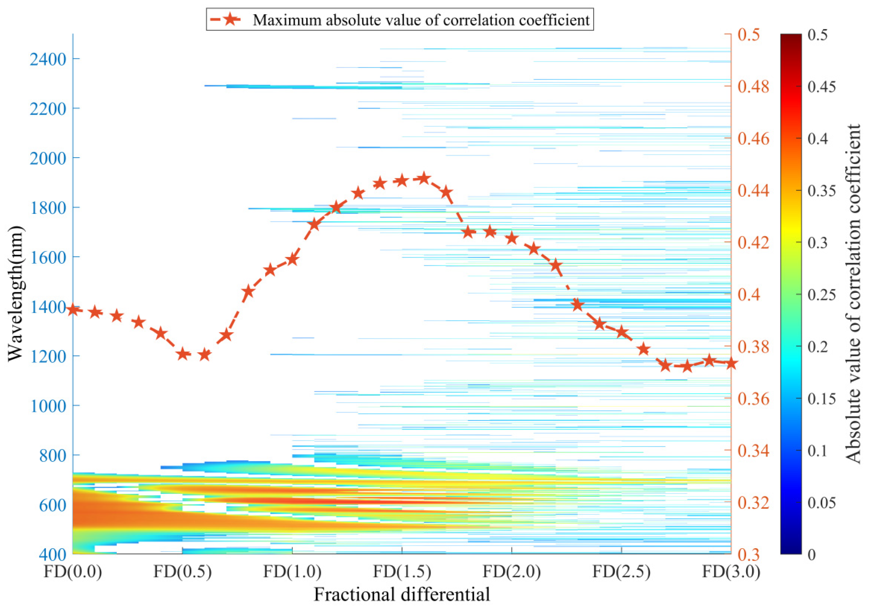
3.1. Leaf N/P Ratio, Fractional Differentiation of Reflectance, and Their Correlation

The mean values of leaf TN, TP, and N/P ratio are 18.51 mg/g, 1.17 mg/g, and 17.97, respectively (Figure 2). The TN content of our study is slightly lower than global and continent levels, with values 20.1 mg/g [44] and 20.20 mg/g [45], respectively. This TP content is significantly lower than the global average of 1.80 mg/g [44] or 1.99 mg/g [46]. The leaf N/P ratio from our study is similar to the results of Yang et al. [47]. The maximum and minimum value of the N/P ratio is 1.34 and 36.94, respectively, with a variation coefficient of 33.68%.

Figure 3 shows the variation of the differential spectral reflectance from 0 to 3 orders. The shape of spectral curves of different orders is smoothly transitional. Compared to integer differentiation (FD (0.0), FD (1.0), FD (2.0), and FD (3.0)), fractional differentiation methods produce more detailed information about the spectrum, and these data subsequently allow for more complex leaf N/P ratio inversion training methods.

The leaf N/P ratio of plants displays a significant correlation with the fractional differential spectra for wavelengths ranging from 400–730 nm (Figure 4). From FD (0) to FD (3), the maximum absolute value of the correlation coefficient displays a unimodal distribution as the fractional differentiation increases from FD (0) to FD (3) with a peak value of 0.44 for FD (1.6).

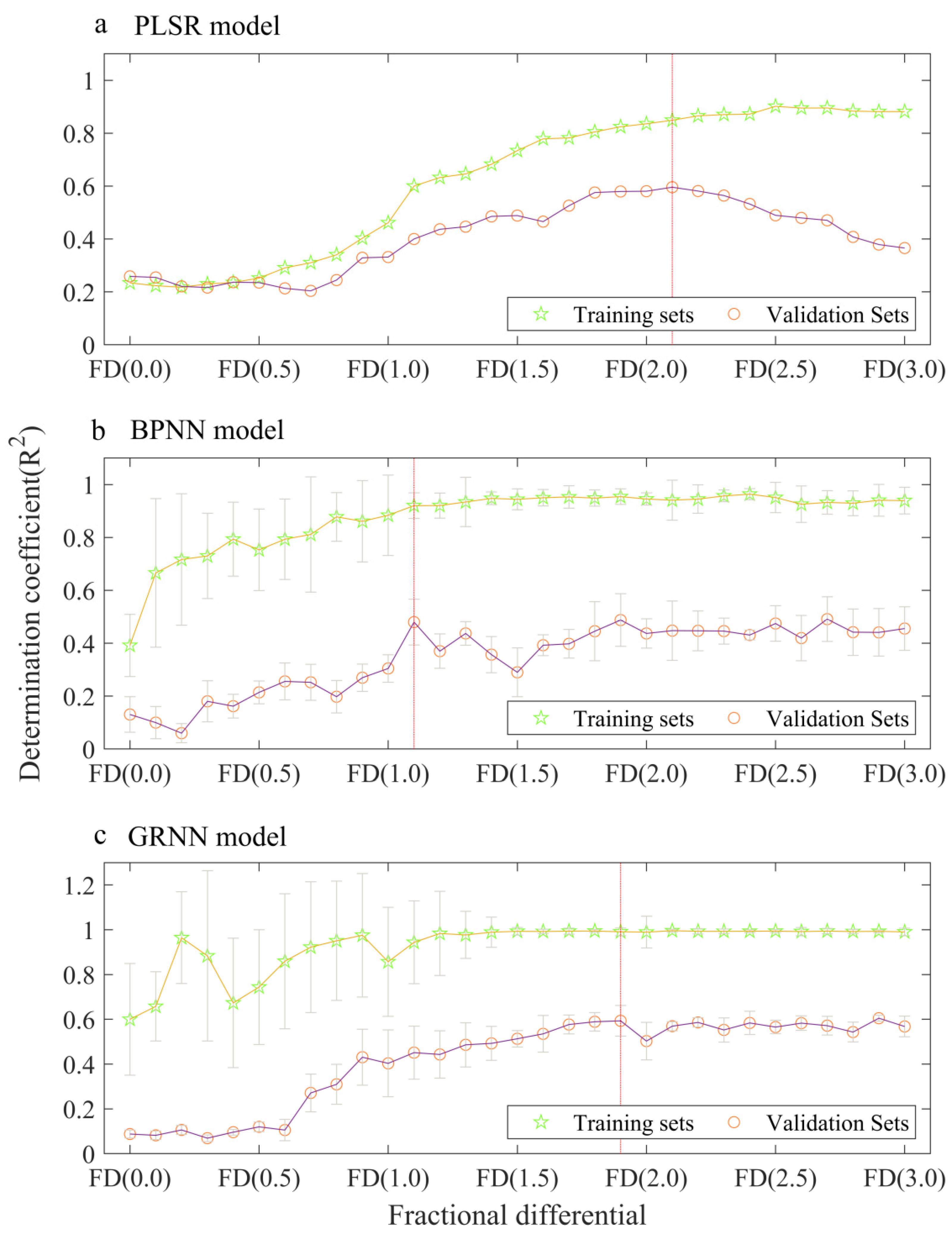
3.2. Performance of a Single Model Using Fractional Differentiation of Reflectance

The accuracy of the PLSR model for predicting leaf N/P ratio of plants continuously increases with increasing fractional order for training sets but displays a unimodal distribution for validation sets (Figure 5a), yielding the highest R² values of 0.66 for FD (2.1). The prediction capability of the PLSR model gradually improves with the increase in fractional order from FD (0.6) to FD (2.1). However, the prediction capability of the PLSR model displayed a higher accuracy in training sets than for validation sets, especially after FD (2.1). This finding suggests that overfitting of the PLSR model is an issue for using this method to predict the leaf N/P ratio of plants.

The accuracy of the BPNN model in predicting the leaf N/P ratio of plants increases with increasing orders of fractional differentiation. The highest R² value for this method is 0.48 for validation sets and 0.92 for training sets around FD (1.1), with values remaining stable across higher fractional orders (Figure 5b). However, the overfitting problem is still present in the BPNN model when predicting the leaf N/P ratio of plants, as shown by the large differences in R² between the training and validation sets.

The value of R² of the GRNN model displays a general increasing trend as the fractional differentiation orders increase between FD (0) and FD (1.2) for training sets and then remain stable (Figure 5c). The R² value for the validation set increases with increasing fractional order from FD (0.0) to FD (1.7). However, similar to the BPNN model, the overfitting problem still exists in the GRNN model, as shown by the differences in the values of R² between training and validation sets.

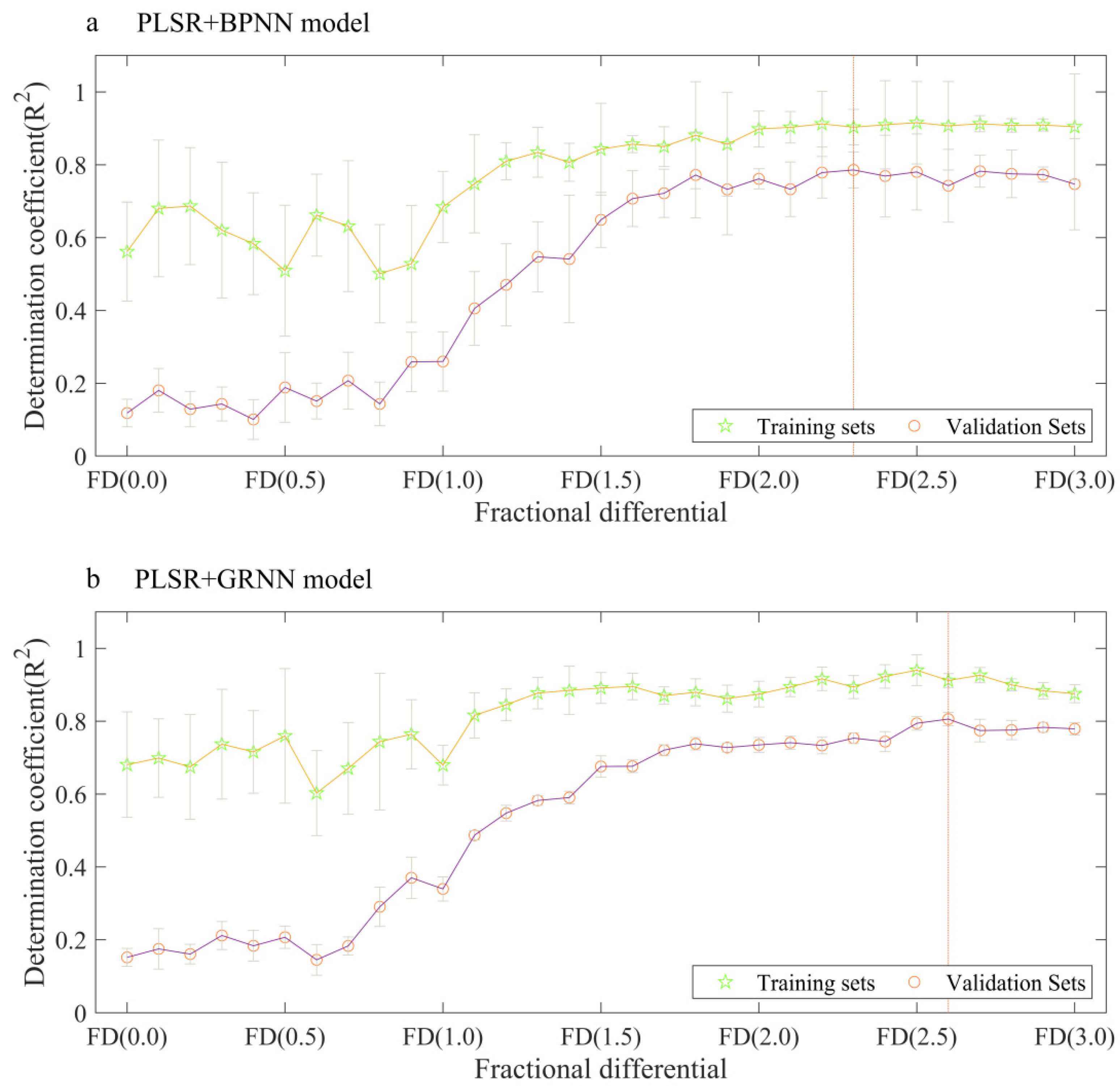
3.3. Performance of Combined Models Using Fractional Differentiation of Reflectance

To overcome the overfitting problem of models in predicting the N/P ratio of plant leaves, a combined model using PLSR+BPNN methods was applied. This PLSR+BPNN model used the principal components extracted from the PLSR model as input variables. The overfitting issue appears to be well-controlled by this method, as shown by the minor differences in R² between the training and validation sets (Figure 6a). The PLSR+BPNN model displays the best performance in predicting the leaf N/P ratio of plants when fractional differentiation was set to FD (2.3), yielding R², RMSE, and RPD values of 0.90, 1.94, and 3.21, respectively, for training sets and 0.79, 2.71, and 2.04 for validation sets (Figure 7).

The combined PLSR+GRNN model also uses principal components extracted from the PLSR model as input variables. When the fractional differential is larger than 1.7, the differences in R² values between the training and validation sets are minor (Figure 6b), suggesting that the overfitting is well-controlled compared to using the PLSR or GRNN models individually. The PLSR+GRNN performed well when the fractional differentiation was set to FD (2.6), with R², RMSE, and RPD values of 0.91, 1.98, and 3.15, respectively, for the training sets, and 0.81, 2.46, and 2.25, respectively, for validation sets (Figure 7).

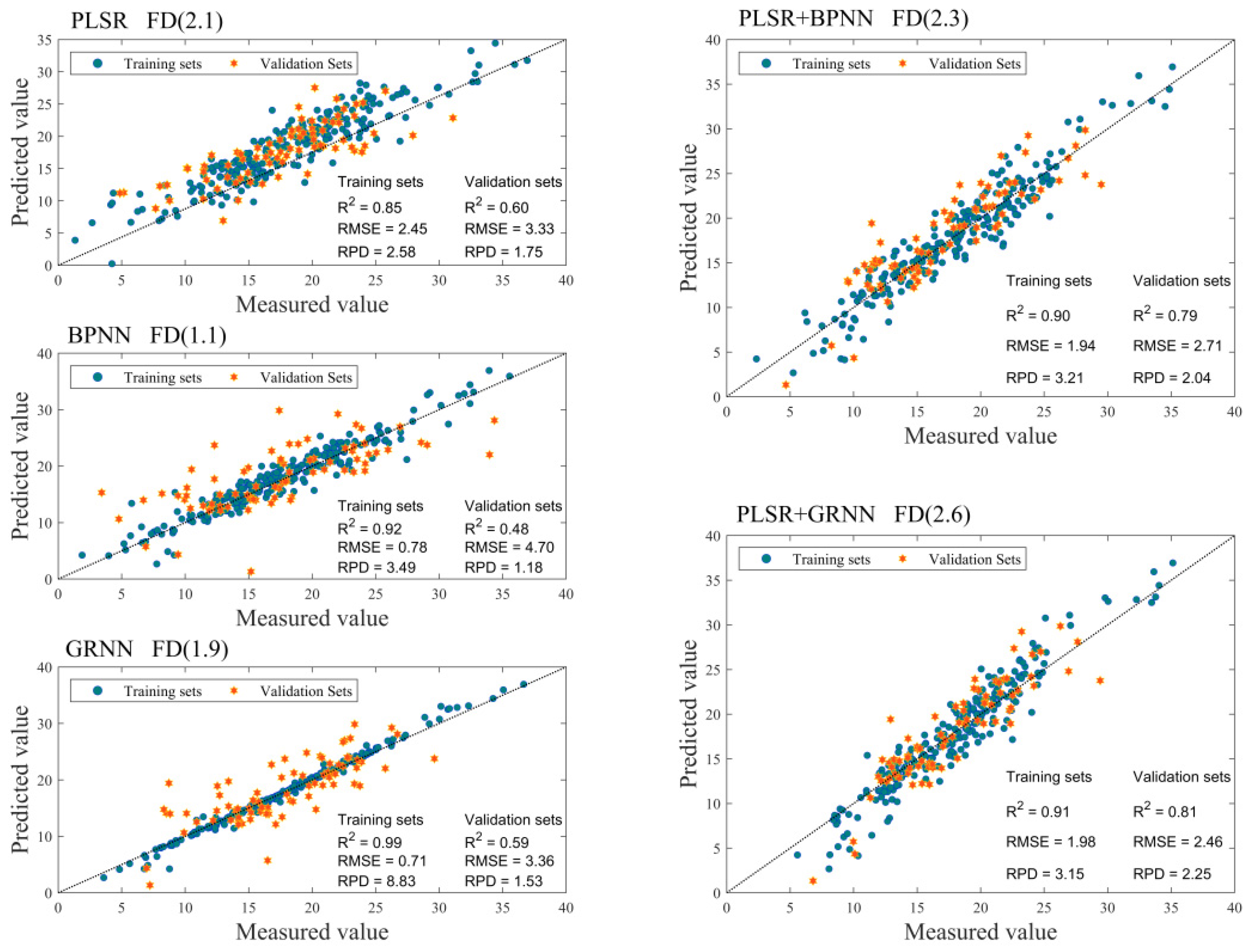
3.4. Model Comparison and Optimal Model Selection

In this study, five models, namely PLSR, BPNN, GRNN, PLSR+BPNN, and PLSR+GRNN, combined with fractional differentiation techniques, were used to predict the leaf N/P ratio of plants in the karst area of Guangxi Province. The optimal fractional differentiation prediction results of each model are shown in Figure 7. The prediction accuracy of these five models can be ranked in descending order as GRNN, BPNN, PLSR+GRNN, PLSR+BPNN, and PLSR according to the coefficient of determination (R²) of the training sets, and PLSR+GRNN, PLSR+BPNN, PLSR, GRNN, and BPNN according to the coefficient of determination (R²) of the validation sets.

The PLSR+BPNN and PLSR+GRNN are excellent models for predicting the leaf N/P ratio of plants in karst area, as they display high prediction accuracy and successfully control overfitting. The PLSR+GRNN model is slightly better than the PLSR+BPNN and is selected as the optimal model in this study.

3.5. Advantages of Fractional Differentiation

Fractional differentiation of spectra can improve the performance of models in predicting the N/P ratio of plant leaves. The optimal differentiation for the five models used in this study is fractional differentiation rather than integer differentiation (

Table 3. Accuracy of optimal fractional differentiation versus integer differentiation.

Model	Orders	Training Sets R2	Training Sets p	Training Sets RMSE	Training Sets RPD	Validation Sets R2	Validation Sets p	Validation Sets RMSE	Validation Sets RPD
PLSR	FD (0.0)	0.23	0.00	5.51	1.15	0.26	0.00	4.51	1.16
	FD (1.0)	0.46	0.00	4.62	1.37	0.33	0.00	4.37	1.19
	FD (2.0)	0.84	0.00	2.55	2.47	0.58	0.00	3.40	1.53
	FD (3.0)	0.88	0.00	2.17	2.91	0.37	0.00	4.32	1.20
	FD (2.1)	0.85	0.00	2.45	2.58	0.60	0.00	3.33	1.57
BPNN	FD (0.0)	0.39	0.00	5.96	1.05	0.13	0.00	8.12	0.68
	FD (1.0)	0.88	0.00	2.25	2.77	0.30	0.00	5.33	1.04
	FD (2.0)	0.95	0.00	1.59	3.91	0.44	0.00	5.03	1.10
	FD (3.0)	0.94	0.00	1.63	3.83	0.46	0.00	4.32	1.28
	FD (1.1)	0.92	0.00	1.78	3.49	0.48	0.00	4.70	1.18
GRNN	FD (0.0)	0.60	0.00	4.43	1.41	0.09	0.01	5.38	1.03
	FD (1.0)	0.86	0.00	3.27	1.91	0.40	0.00	4.37	1.26
	FD (2.0)	0.99	0.00	0.86	7.20	0.50	0.00	4.33	1.28
	FD (3.0)	0.99	0.00	0.83	7.54	0.57	0.00	3.69	1.50
	FD (1.9)	0.99	0.00	0.71	8.83	0.59	0.00	3.61	1.53
PLSR+BPNN	FD (0.0)	0.56	0.00	4.13	1.51	0.12	0.00	5.67	0.98
	FD (1.0)	0.68	0.00	3.54	1.76	0.26	0.00	5.08	1.09
	FD (2.0)	0.90	0.00	2.00	3.11	0.76	0.00	2.78	1.99
	FD (3.0)	0.90	0.00	2.03	3.07	0.75	0.00	3.01	1.84
	FD (2.3)	0.90	0.00	1.94	3.21	0.79	0.00	2.71	2.04
PLSR+GRNN	FD (0.0)	0.68	0.00	3.95	1.58	0.80	0.00	5.08	1.09
	FD (1.0)	0.68	0.00	3.87	1.61	0.80	0.00	4.49	1.23
	FD (2.0)	0.87	0.00	2.44	2.56	0.80	0.00	2.86	1.93
	FD (3.0)	0.88	0.00	2.36	2.64	0.80	0.00	2.67	2.07
	FD (2.6)	0.91	0.00	1.98	3.15	0.81	0.00	2.46	2.25

). For example, the best fractional differentiation of the PLSR model is FD (2.1), with an RPD of 2.45 for the training sets and an RPD of 1.57 for the validation sets. The PLSR model with a fractional differentiation of 2.1 produced more accurate and robust values than zero, first, second, and third orders differentiation. Additionally, the optimal fractional differentiation of the PLSR+BPNN model and the PLSR+GRNN model is FD (2.3) and FD (2.6), respectively, which both produce better values than zero, first, second, and third orders differentiation. These results suggest that the fractional differential transform plays a positive role in predicting the leaf N/P ratio of plants.

4. Discussion

4.1. Distribution of Sensitive Wavelengths

The spectral reflectance from 400–730 nm, and especially 520–650 nm, are sensitive wavelengths for predicting the leaf N/P ratio of plants. This result is consistent with previous studies, such as Cui et al. [8], who found that near 650 nm was the best wavelength for estimating the N/P ratio. Hansen and Schjoerring [48] also showed that spectral reflectance near 530 nm and 720 nm are important wavelengths for estimating the N concentration of wheat. In addition, Xu et al. [49] found that spectral reflectance of 540–560 nm and 760–780 nm are sensitive wavelengths for the C/N ratio of wheat and barley leaves. There are some differences in sensitive wavelengths related to the leaf N/P ratio between the karst and non-karst plants, which may be caused by adaptions to survive in karst environments. For example, plants growing in karst areas have decreased stomatal conductance, thickened palisade tissue, and increased keratinization due to thin soil layers and relatively low air humidity [50]. These physiological differences can impact the radiative transfer processes of plant leaves, leading to changes in the sensitive wavebands.

4.2. Control Overfitting

We reduced the noise in the spectral reflectance by fractional differentiation and improved the representativeness of the feature variables for the model input. Moreover, we applied the PLSR model to extract principal components to reduce the dimensionality of the spectral data. The reduced-dimensional spectral data are used as input variables of the BPNN and GRNN models. In this way, we proposed two composite models, PLSR+BPNN and PLSR+GRNN. The prediction performance of PLSR+BPNN and PLSR+GRNN models will be better than simple models such as spectral index and ordinary linear regression. The simple model is more adapted to a single plant species [14,51,52] and very sensitive to databases [16]. In contrast, our model is more adaptable to complex environments as it is set up in a mixed forest database. On the other hand, this method decreases the complexity of the model while ensuring minimal loss of spectral information and reducing the occurrence of overfitting. These results are consistent with previous studies [53] that show overfitting issues could be overcome by using non-negative principal component analysis (NPCA) to extract principal components as input variables for machine learning. Although combining PCA or PLSR models with machine learning methods does not help improve the model prediction capability, it effectively minimizes the overfitting problem of machine learning methods.

4.3. Application for Mixed Forest

Empirical models tend to be site-, time-, and species-specific and are therefore unsuitable for large-scale analyses [54]. Previous studies investigating the inversion of plant biochemical parameters are also biased towards specific regions, such as wetlands [24] or grasslands [28], or species such as wheat [55] or rice [17]. Although high accuracy can be obtained from the inversion of biochemical parameters for a single species [15], plants are more likely to co-exist in a mixed form in the natural environment, and studies on only one species are not applicable to diverse ecosystems. Studies across various species need to be conducted before these methods can be applied to mixed forest environments. However, it is crucial to improve the model accuracy and robustness before the inversion of biochemical parameters of mixed species. We applied five models to predict the leaf N/P ratio of plants in a karst area. Among them, the PLSR+BPNN and PLSR+GRNN models have the best performance, with high prediction accuracy and robustness. The performance of both the PLSR+BPNN and PLSR+GRNN models was better than the models used by Cheng et al. [16] in terms of the coefficient of determination (R²). This improved performance is mainly due to the full consideration of both linear and nonlinear relationships between leaf biochemical parameters and field spectroradiometer data in our study.

Sample composition also impacts the model performance. For example, there was a significant difference in the performance of the BPNN model between our study and Cui et al. [8] when comparing the coefficient of determination for validation tests, and no overfitting was observed in the results of Cui et al. [8]. These differences in performance were due to the large variability in sample composition, with leaf N/P ratio of plants in this study ranging from 1.34 to 36.94 compared to that of phragmites communis N/P ratio ranging from 6.7 to 15.9 in the Cui et al. study [8].

5. Conclusions

Estimating the N/P ratio of plant leaves using field spectroradiometer data is challenging. We estimated the variation of leaf N/P ratio of plants in a karst area of Guangxi Province using five models, namely PLSR, BPNN, GRNN, PLSR+BPNN, and PLSR+GRNN. The sensitivity wavelengths of the leaf N/P ratio of plants are mainly in the range of 400–730 nm. Applying a single model (such as PLSR, or BPNN, and or GRNN) can estimate the leaf N/P ratio of plants, but all methods produce significant overfitting of the data. In contrast, the combined models of PLSR+BPNN and PLSR+GRNN can avoid the overfitting problem in predicting the leaf N/P ratio of plants, and have high accuracy prediction capabilities. In addition, using fractional differentiation methods can effectively improve the prediction capability of the model in estimating the leaf N/P ratio across a variety of plant species. This study provides a valuable scientific basis for long-term dynamic monitoring of plant biochemical parameters using field spectroradiometer data.

References

1. Vrede, T.; Dobberfuhl, D.R.; Kooijman, S.A.L.M.; Elser, J.J. Fundamental connections among organism C: N: P stoichiometry, macromolecular composition, and growth. Ecology 2004, 85, 1217–1229. [Google Scholar] [CrossRef] [Green Version]
2. Elser, J.J.; Sterner, R.W.; Gorokhova, E.; Fagan, W.F.; Markow, T.A.; Cotner, J.B.; Harrison, J.F.; Hobbie, S.E.; Odell, G.M.; Weider, L.W. Biological stoichiometry from genes to ecosystems. Ecol. Lett. 2000, 3, 540–550. [Google Scholar] [CrossRef] [Green Version]
3. Liu, J.; Gou, X.; Zhang, F.; Bian, R.; Yin, D. Spatial patterns in the C: N: P stoichiometry in Qinghai spruce and the soil across the Qilian Mountains, China. Catena 2020, 196, 104814. [Google Scholar] [CrossRef]
4. Elser, J.J.; Fagan, W.F.; Kerkhoff, A.J.; Swenson, N.G.; Enquist, B.J. Biological stoichiometry of plant production: Metabolism, scaling and ecological response to global change. New Phytol. 2010, 186, 593–608. [Google Scholar] [CrossRef] [Green Version]
5. Batterman, S.A.; Wurzburger, N.; Hedin, L.O.; Austin, A. Nitrogen and phosphorus interact to control tropical symbiotic N2 fixation: A test inInga punctata. J. Ecol. 2013, 101, 1400–1408. [Google Scholar] [CrossRef]
6. Koerselman, W.; Meuleman, A.M.F. The Vegetation N: P Ratio: A New Tool to Detect the Nature of Nutrient Limitation. J. Appl. Ecol. 1996, 33, 1441–1450. [Google Scholar] [CrossRef]
7. Gusewell, S. Variation in nitrogen and phosphorus concentrations of wetland plants. Perspect. Plant Ecol. Evol. Syst. 2002, 5, 37–61. [Google Scholar] [CrossRef]
8. Cui, L.; Dou, Z.; Liu, Z.; Zuo, X.; Lei, Y.; Li, J.; Zhao, X.; Zhai, X.; Pan, X.; Li, W. Hyperspectral inversion of phragmites communis carbon, nitrogen, and phosphorus stoichiometry using three models. Remote Sens. 2020, 12, 1998. [Google Scholar] [CrossRef]
9. Rei, S.; Quan, W. Towards a Universal Hyperspectral Index to Assess Chlorophyll Content in Deciduous Forests. Remote Sens. 2017, 9, 191. [Google Scholar]
10. Zhao, H.S.; Zhu, X.C.; Li, C.; Wei, Y.; Zhao, G.X.; Jiang, Y.M. Improving the accuracy of the hyperspectral model for apple canopy water content prediction using the equidistant sampling method. Sci. Rep. 2017, 7, 11192. [Google Scholar] [CrossRef] [PubMed] [Green Version]
11. Yamashita, H.; Sonobe, R.; Hirono, Y.; Morita, A.; Ikka, T. Dissection of hyperspectral reflectance to estimate nitrogen and chlorophyll contents in tea leaves based on machine learning algorithms. Sci. Rep. 2020, 10, 17360. [Google Scholar] [CrossRef]
12. Barnaby, J.Y.; Huggins, T.D.; Lee, H.; McClung, A.M.; Pinson, S.R.M.; Oh, M.; Bauchan, G.R.; Tarpley, L.; Lee, K.; Kim, M.S.; et al. Vis/NIR hyperspectral imaging distinguishes sub-population, production environment, and physicochemical grain properties in rice. Sci. Rep. 2020, 10, 9284. [Google Scholar] [CrossRef]
13. El-Hendawy, S.; Al-Suhaibani, N.; Alotaibi, M.; Hassan, W.; Elsayed, S.; Tahir, M.U.; Mohamed, A.I.; Schmidhalter, U. Estimating growth and photosynthetic properties of wheat grown in simulated saline field conditions using hyperspectral reflectance sensing and multivariate analysis. Sci. Rep. 2019, 9, 16473. [Google Scholar] [CrossRef]
14. Meacham-Hensold, K.; Montes, C.M.; Wu, J.; Guan, K.; Fu, P.; Ainsworth, E.A.; Pederson, T.; Moore, C.E.; Brown, K.L.; Raines, C.; et al. High-throughput field phenotyping using hyperspectral reflectance and partial least squares regression (PLSR) reveals genetic modifications to photosynthetic capacity. Remote Sens. Environ. 2019, 231, 111176. [Google Scholar] [CrossRef] [PubMed]
15. Sonobe, R.; Hirono, Y.; Oi, A. Non-destructive detection of tea leaf chlorophyll content using hyperspectral reflectance and machine learning algorithms. Plants 2020, 9, 368. [Google Scholar] [CrossRef] [Green Version]
16. Cheng, T.; Rivard, B.; Sánchez-Azofeifa, A.G.; Féret, J.-B.; Jacquemoud, S.; Ustin, S.L. Deriving leaf mass per area (LMA) from foliar reflectance across a variety of plant species using continuous wavelet analysis. ISPRS J. Photogramm. Remote Sens. 2014, 87, 28–38. [Google Scholar] [CrossRef]
17. Inoue, Y.; Sakaiya, E.; Zhu, Y.; Takahashi, W. Diagnostic mapping of canopy nitrogen content in rice based on hyperspectral measurements. Remote Sens. Environ. 2012, 126, 210–221. [Google Scholar] [CrossRef]
18. Doktor, D.; Lausch, A.; Spengler, D.; Thurner, M. Extraction of plant physiological status from hyperspectral signatures using machine learning methods. Remote Sens. 2014, 6, 12247–12274. [Google Scholar] [CrossRef] [Green Version]
19. Oh, K.; Chung, Y.C.; Kim, K.W.; Kim, W.S.; Oh, I.S. Classification and visualization of Alzheimer’s disease using volumetric convolutional neural network and transfer learning. Sci. Rep. 2019, 9, 18150. [Google Scholar] [CrossRef]
20. Gansfort, B.; Traunspurger, W. Environmental factors and river network position allow prediction of benthic community assemblies: A model of nematode metacommunities. Sci. Rep. 2019, 9, 14716. [Google Scholar] [CrossRef] [Green Version]
21. Sengupta, D.; Bandyopadhyay, S.; Sinha, D. A scoring scheme for online feature selection: Simulating model performance without retraining. IEEE Trans. Neural Netw. Learn. Syst. 2017, 28, 405–414. [Google Scholar] [CrossRef]
22. Cheng, Q.; Zhou, H.; Cheng, J. The fisher-markov selector: Fast selecting maximally separable feature subset for multiclass classification with applications to high-dimensional data. IEEE Trans. Pattern Anal. Mach. Intell. 2010, 33, 1217–1233. [Google Scholar] [CrossRef]
23. Barzegar, R.; Moghaddam, A.A.; Deo, R.; Fijani, E.; Tziritis, E. Mapping groundwater contamination risk of multiple aquifers using multi-model ensemble of machine learning algorithms. Sci. Total Environ. 2018, 621, 697–712. [Google Scholar] [CrossRef]
24. Dou, Z.; Li, Y.; Cui, L.; Pan, X.; Ma, Q.; Huang, Y.; Lei, Y.; Li, J.; Zhao, X.; Li, W. Hyperspectral inversion of Suaeda salsa bi omass under different types of human activity in Liaohe Estuary wetland in north-eastern China. MAR Freshw. Res. 2020, 71, 482–492. [Google Scholar] [CrossRef]
25. Guo, C.; Guo, X. Estimating leaf chlorophyll and nitrogen content of wetland emergent plants using hyperspectral data in the visible domain. Spectrosc. Lett. 2015, 49, 180–187. [Google Scholar] [CrossRef]
26. Peuelas, J.; Gamon, J.A.; Fredeen, A.L.; Merino, J.; Field, C.B. Reflectance indices associated with physiological changes in nitrogen- and water-limited sunflower leaves. Remote Sens. Environ. 1994, 48, 135–146. [Google Scholar] [CrossRef]
27. Benkhettou, N.; Brito da Cruz, A.M.C.; Torres, D.F.M. A fractional calculus on arbitrary time scales: Fractional differentiation and fractional integration. Sig. Process. 2015, 107, 230–237. [Google Scholar] [CrossRef] [Green Version]
28. Gao, J.; Liu, J.; Liang, T.; Hou, M.; Ge, J.; Feng, Q.; Wu, C.; Li, W. Mapping the forage nitrogen-phosphorus ratio based on Sentinel-2 MSI data and a random forest algorithm in an alpine grassland ecosystem of the Tibetan Plateau. Remote Sens. 2020, 12, 2929. [Google Scholar] [CrossRef]
29. Yuan, D. World correlation of karst ecosystem: Objectives and implementation plan. China Adv. Earth Sci. 2001, 4, 461–466. (In Chinese) [Google Scholar]
30. Luo, Z.; Tang, S.; Jiang, Z.; Chen, J.; Fang, H.; Li, C. Conservation of terrestrial vertebrates in a global hotspot of karst area in southwestern China. Sci. Rep. 2016, 6, 25717. [Google Scholar] [CrossRef] [Green Version]
31. Orme, C.D.; Davies, R.G.; Burgess, M.; Eigenbrod, F.; Pickup, N.; Olson, V.A.; Webster, A.J.; Ding, T.S.; Rasmussen, P.C.; Ridgely, R.S.; et al. Global hotspots of species richness are not congruent with endemism or threat. Nature 2005, 436, 1016–1019. [Google Scholar] [CrossRef]
32. Zeng, F.; Peng, W.; Song, T.; Wang, K.; Wu, H.; Song, X.; Zeng, Z. Changes in vegetation after 22 years’ natural restoration in the karst disturbed area in northwestern Guangxi, China. Acta Ecol. Sin. 2007, 27, 5110–5119. [Google Scholar] [CrossRef]
33. SU, Z.; LI, X. The types of natural vegetation in karst region of Guangxi and its classified system. Guihaia 2003, 23, 289–293. [Google Scholar]
34. Shimadzu, S.; Seo, M.; Terashima, I.; Yamori, W. Whole irradiated plant leaves showed faster photosynthetic induction than individually irradiated leaves via improved stomatal opening. Front. Plant Sci. 2019, 10, 1512. [Google Scholar] [CrossRef] [PubMed] [Green Version]
35. Richard, H.L.; Donald, L.S. Soil Science of America and American Society of Agronomy. In Methods of Soil Analysis. Part 3. Chemical Methods; Soil Science Society of America: Madison, WI, USA, 1996; pp. 1085–1121. [Google Scholar]
36. Bao, S.D. Soil and Agricultural Chemistry Analysis; Agriculture Publication: Beijing, China, 2000; pp. 71–79. [Google Scholar]
37. Kharintsev, S.S.; Salakhov, M. A simple method to extract spectral parameters using fractional derivative spectrometry. Spectrochim. Acta A Mol. Biomol. Spectrosc. 2004, 60, 2125–2133. [Google Scholar] [CrossRef] [PubMed]
38. Han, Z.; Li, S.; Liu, H. Composite learning sliding mode synchronization of chaotic fractional-order neural networks. J. Adv. Res. 2020, 25, 87–96. [Google Scholar] [CrossRef] [PubMed]
39. Rumelhart, D.E.; Hinton, G.E.; Williams, R.J. Learning representations by back-propagating errors. Nature 1986, 323, 533–536. [Google Scholar] [CrossRef]
40. Stathakis, D. How many hidden layers and nodes? Int. J. Remote Sens. 2009, 30, 2133–2147. [Google Scholar] [CrossRef]
41. Specht, D.F. A general regression neural network. IEEE Trans. Neural Netw. 1991, 2, 568–576. [Google Scholar] [CrossRef] [Green Version]
42. Lotfinejad, M.; Hafezi, R.; Khanali, M.; Hosseini, S.; Mehrpooya, M.; Shamshirband, S. A comparative assessment of predicting daily solar radiation using bat neural network (BNN), generalized regression neural network (GRNN), and neuro-fuzzy (NF) system: A case study. Energies 2018, 11, 1188. [Google Scholar] [CrossRef] [Green Version]
43. Chang, C.-W.; Laird, D.A.; Mausbach, M.J.; Hurburgh, C.R. Near-infrared reflectance spectroscopy–principal components regression analyses of soil properties. Soil Sci. Soc. Am. J. 2001, 65, 480–490. [Google Scholar] [CrossRef] [Green Version]
44. Reich, P.B.; Oleksyn, J. Global patterns of plant leaf N and P in relation to temperature and latitude. Proc. Natl. Acad. Sci. USA 2004, 101, 11001–11006. [Google Scholar] [CrossRef] [Green Version]
45. Han, W.; Fang, J.; Guo, D.; Zhang, Y. Leaf nitrogen and phosphorus stoichiometry across 753 terrestrial plant species in China. New Phytol. 2005, 168, 377–385. [Google Scholar] [CrossRef] [PubMed]
46. Elser, J.J.; Fagan, W.F.; Denno, R.F.; Dobberfuhl, D.R.; Folarin, A.; Huberty, A.; Interlandi, S.; Kilham, S.S.; McCauley, E.; Schulz, K.L. Nutritional constraints in terrestrial and freshwater food webs. Nature 2000, 408, 578–580. [Google Scholar] [CrossRef] [PubMed]
47. Yang, H.; Li, Q.; Tu, C.; Cao, J. Carbon, nitrogen and phosphorus stoichiometry of typical plants in karst area of Maocun, Guilin. Guangxi Zhiwu/Guihaia 2015, 35, 493–555. [Google Scholar]
48. Hansen, P.M.; Schjoerring, J.K. Reflectance measurement of canopy biomass and nitrogen status in wheat crops using normalized difference vegetation indices and partial least squares regression. Remote Sens. Environ. 2003, 86, 542–553. [Google Scholar] [CrossRef]
49. Xu, X.; Yang, G.; Yang, X.; Li, Z.; Feng, H.; Xu, B.; Zhao, X. Monitoring ratio of carbon to nitrogen (C/N) in wheat and barley leaves by using spectral slope features with branch-and-bound algorithm. Sci. Rep. 2018, 8, 10034. [Google Scholar] [CrossRef]
50. Li, R.; Wang, S.; Du Xuelian, Y.G. Relationship among leaf anatomical characters and foliarδ~ (13) C values of six woody species for karst rocky desertification areas. China Sci. Silvae Sin. 2008, 44, 29–34. [Google Scholar]
51. Liu, X.; Guanter, L.; Liu, L.; Damm, A.; Malenovský, Z.; Rascher, U.; Peng, D.; Du, S.; Gastellu-Etchegorry, J.-P. Downscaling of solar-induced chlorophyll fluorescence from canopy level to photosystem level using a random forest model. Remote Sens. Environ. 2018, 231, 110772. [Google Scholar] [CrossRef]
52. Jay, S.; Maupas, F.; Bendoula, R.; Gorretta, N. Retrieving LAI, chlorophyll and nitrogen contents in sugar beet crops from multi-angular optical remote sensing: Comparison of vegetation indices and PROSAIL inversion for field phenotyping. Field Crop. Res. 2017, 210, 33–46. [Google Scholar] [CrossRef] [Green Version]
53. Han, X. Nonnegative principal component analysis for cancer molecular pattern discovery. IEEE/ACM Trans. Comput. Biol. Bioinform. 2010, 7, 537–549. [Google Scholar] [PubMed]
54. Zhu, Z.; Bi, J.; Pan, Y.; Ganguly, S.; Anav, A.; Xu, L.; Samanta, A.; Piao, S.; Nemani, R.; Myneni, R. Global data sets of vegetation leaf area index (LAI) 3g and fraction of photosynthetically active radiation (FPAR) 3g derived from global inventory modeling and mapping studies (GIMMS) normalized difference vegetation index (NDVI 3g) for the period 1981 to 2011. Remote Sens. 2013, 5, 927–948. [Google Scholar]
55. Camino, C.; Gonzalez-Dugo, V.; Hernandez, P.; Zarco-Tejada, P.J. Radiative transfer Vcmax estimation from hyperspectral imagery and SIF retrievals to assess photosynthetic performance in rainfed and irrigated plant phenotyping trials. Remote Sens. Environ. 2019, 231, 111186. [Google Scholar] [CrossRef]
Figure 1. Location of the nine study plots.
Remotesensing 13 03368 g001
Figure 2. The leaf N/P ratio frequency distribution. TN-mean, TP-mean, and N/P-mean are the mean values of total nitrogen, total phosphorus, and N/P ratio, respectively. N/P-minimum, N/P-maximum, N/P-std, N/P-cv, and N/P-ks are the N/P ratio minimum, maximum, standard deviation, coefficient of variation, and one-sample Kolmogorov–Smirnov test, respectively. n is the number of samples.
Remotesensing 13 03368 g002
Figure 3. Fractional differential curves of plant leaf spectral reflectance (average of all the collected samples). If the curves overlap, the former will be overwritten by the latter.
Remotesensing 13 03368 g003
Figure 4. Distribution for the absolute values of correlation coefficients between fractional differentiation spectra and N/P ratio (vertical axis on the left side) and the maximum absolute value of each order fractional differentiation correlation coefficient (vertical axis on the right side). The color bar indicates the magnitude of the correlation coefficient. The white areas of the graph show where the spectral bands did not pass the 0.05 significance test.
Remotesensing 13 03368 g004
Figure 5. Trends of single model ((a) is the PLSR model, (b) is the BPNN model, and (c) is the GRNN model) methods from zero to third order of fractional differentiation R2. The error bars represent two standard errors of each estimate, where available. The red vertical line indicates the position of the optimal fractional differentiation.
Remotesensing 13 03368 g005
Figure 6. Trends of the differentiation coefficient (R2) for combined model ((a) is the PLSR+BPNN model and (b) is the PLSR+GRNN model) methods. The error bars represent two standard errors of each estimate. The red vertical line indicates the position of the optimal fractional differentiation.
Remotesensing 13 03368 g006
Figure 7. Leaf N/P ratio prediction accuracy of optimal fractional differentiation for each model (p < 0.01).
Remotesensing 13 03368 g007