Article

Spatio-Temporal Variation Characteristics of Aboveground Biomass in the Headwater of the Yellow River Based on Machine Learning

1
State Key Laboratory of Grassland Agro-Ecosystems, College of Pastoral Agriculture Science and Technology, Lanzhou University, Lanzhou 730000, China
2
Key Laboratory of Grassland Livestock Industry Innovation, College of Pastoral Agriculture Science and Technology, Lanzhou University, Lanzhou 730000, China
*
Author to whom correspondence should be addressed.
Remote Sens. 2021, 13(17), 3404; https://doi.org/10.3390/rs13173404
Submission received: 26 July 2021 / Revised: 23 August 2021 / Accepted: 24 August 2021 / Published: 27 August 2021

Abstract

:
Accurate estimation of the aboveground biomass (AGB) of grassland is a key link in understanding the regional carbon cycle. We used 501 aboveground measurements, 29 environmental variables, and machine learning algorithms to construct and verify a custom model of grassland biomass in the Headwater of the Yellow River (HYR) and selected the random forest model to analyze the temporal and spatial distribution characteristics and dynamic trends of the biomass in the HYR from 2001 to 2020. The research results show that: (1) the random forest model is superior to the other three models (R2val = 0.56, RMSEval = 51.3 g/m2); (2) the aboveground biomass in the HYR decreases spatially from southeast to northwest, and the annual average value and total values are 176.8 g/m2 and 20.73 Tg, respectively; (3) 69.51% of the area has shown an increasing trend and 30.14% of the area showed a downward trend, mainly concentrated in the southeast of Hongyuan County, the northeast of Aba County, and the north of Qumalai County. The research results can provide accurate spatial data and scientific basis for the protection of grassland resources in the HYR.

Graphical Abstract

1. Introduction

The grassland ecosystem is the largest terrestrial biosystem on the earth’s surface, accounting for about 40% of the total land area [1], and plays an important role in global carbon cycle and climate regulation [2]. Grassland plays a role in modulating climate, wind-resistant sand, maintaining soil and ecological balance, and the economic development of the pastoral area, thus maintaining the sustainable development of animal husbandry [3,4]. The current status and changing trend of grassland aboveground biomass reflects whether the utilization of grassland is scientific and reasonable, which is the focus of ecological environment protection and the sustainable development of animal husbandry [5,6].
The aboveground biomass (AGB) can be predicted by direct methods (by harvesting the biomass) and by indirect methods (including the use of remote sensing tools). The direct harvest method is more accurate in a small area, but it is time-consuming and labor-intensive, difficult to achieve on a large-scale and long-term sequence, and will cause certain ecological damage to the grassland [7]. In contrast, remote sensing technology has low-cost and can monitor the current status and dynamic changes of grassland resources. In the 1980s, NOAA/AVHRR data were used, by previous authors, to estimate grassland production in grasslands. Diallo et al. [8] used AVHRR data to predict natural grasslands in the Sahel region of Africa. In recent years, the method of establishing a biomass statistical regression model through the vegetation index is widely used. The vegetation index most commonly used for aboveground biomass monitoring is the normalized difference vegetation index (NDVI), but it has many problems [9], such as saturation and the impact on the soil background in low vegetation coverage areas. Therefore, scholars have proposed other vegetation indexes, such as EVI, MSAVI, NDVGI, SAVI, etc. Different vegetation indexes have their own characteristics, and it is difficult to prove which vegetation index is superior. Statistical models are divided into parametric and non-parametric models. According to different regression variables, parameter models can be divided into linear and nonlinear regression models. Paruelo et al. [10] combined NDVI data with the measured biomass on the ground to monitor the grassland biomass in the grasslands of the central United States and found that the power function regression model is more suitable for local biomass monitoring than the linear regression model. The simple one-dimensional curve model is usually unable to achieve the high-precision fitting of biomass, while multivariate linear simulations do not allow for large correlations between variables; otherwise, it will cause multicollinearity problems and affect the modeling effect. Because there are often significant correlations between vegetation indices, it is difficult for multiple linear models to accurately estimate biomass.
There are many vegetation indices that can be used for AGB estimation; however, the variation of AGB is not only influenced by a single factor but also by a variety of factors, such as soil, climate, and topography factor, etc. In previous studies, estimating AGB using only a single type of factor may have introduced errors and uncertainty. Idowu et al. [11] found that for models with a non-unique number of variables, machine learning algorithms may be more effective than ordinary regression models. Machine learning methods, such as random forest (RF) regression, can integrate multiple factors and learn highly complex nonlinear mappings for estimating AGB. Wang et al. [12] estimated the AGB of the Loess Plateau using the RF algorithm, combining 233 field observations and their corresponding climate and remote sensing data from 2011–2013, and compared the two methods, showing better accuracy from the neural network, compared to the multiple linear regression model. Xie et al. [13] used neural network model and multiple linear regression model to estimate the aboveground biomass of grassland and compared the two methods. The neural network model is better than the multiple linear. Research by Yang et al. [14] showed that the accuracy of the BP-ANN model for grassland AGB inversion was significantly higher than that of the traditional multi-factor inversion model in the THR. Zeng et al. [4] developed an AGB estimation model suitable for the Qinghai-Tibet Plateau, based on the random forest algorithm. The R2 of the model is equal to 0.86.
The HYR is located in the northeastern part of the Qinghai-Tibet Plateau, which is called “the water tower of the Yellow River” [15]. In recent years, desertification, due to overgrazing and other grassland problems, has become more and more serious. Effective monitoring of regional grassland is an urgent problem to be solved. Achieving the rapid and effective monitoring of grassland changes is not only an urgent need, to determine a reasonable grassland stock carrying capacity, but also a realistic need to ensure the development of animal husbandry. Measured data are the key parameter for constructing the optimal model in this study. The reasonable setting of sample points will directly affect the results of model simulation [16]. The high altitude, harsh natural conditions, inaccessibility, high mountains, and wetlands in the HYR made the collection of samples difficult. Therefore, the distribution of sample points should be representative of the general characteristics of the HYR, but also take into account the difficulty of sample collection and sampling costs.
The study uses 501 measured AGB data, combined with factors for climate, vegetation indices, soil texture, and topography, to construct a data set of environmental variables affecting AGB in the HYR. The main goals are: (1) comparing and analyzing the accuracy of various machine learning model algorithms to build an inversion model suitable for estimating grassland AGB in the HYR; (2) simulate the spatial distribution and temporal trend of grassland AGB in the HYR from 2001 to 2020.

2. Materials and Methods
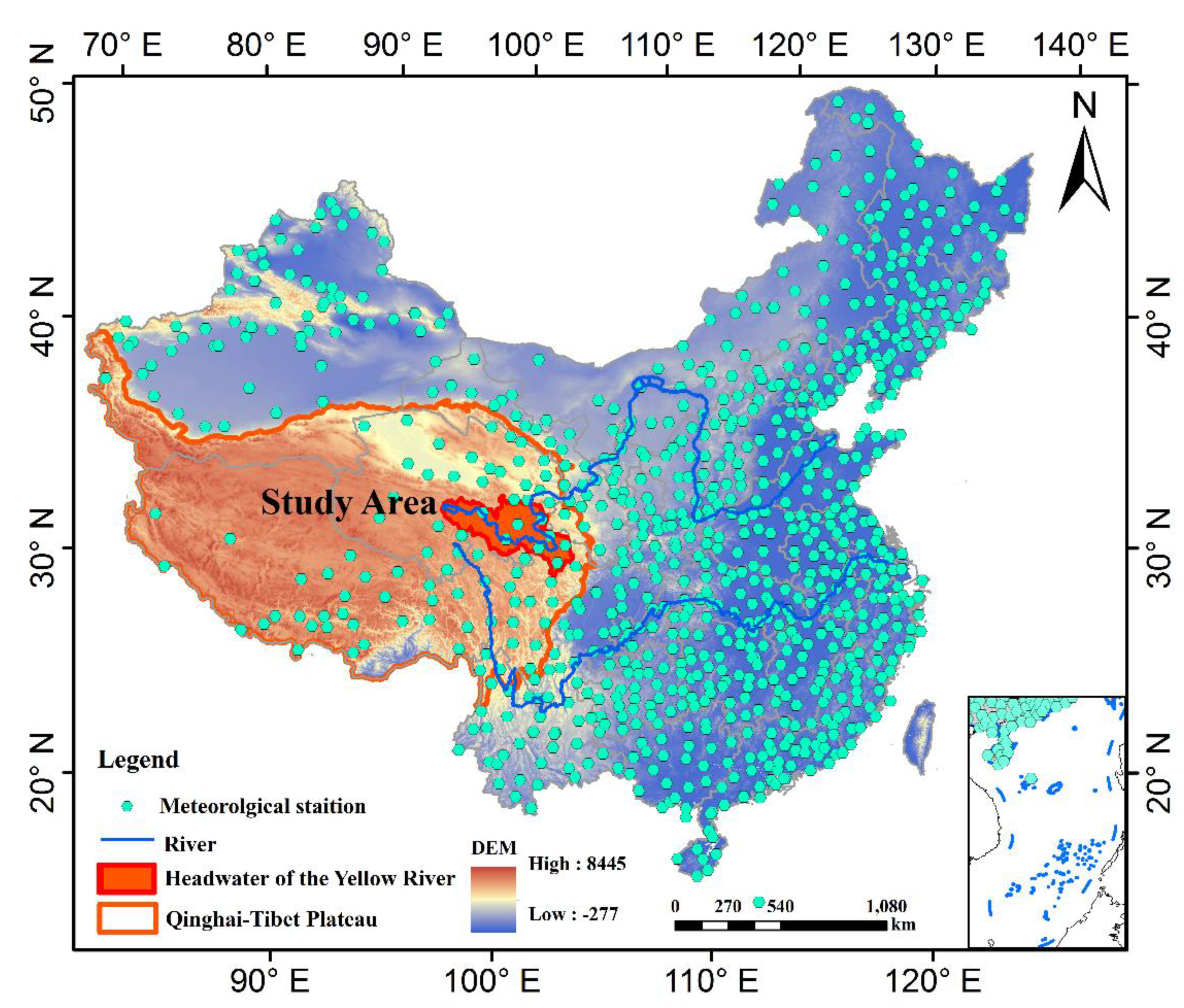
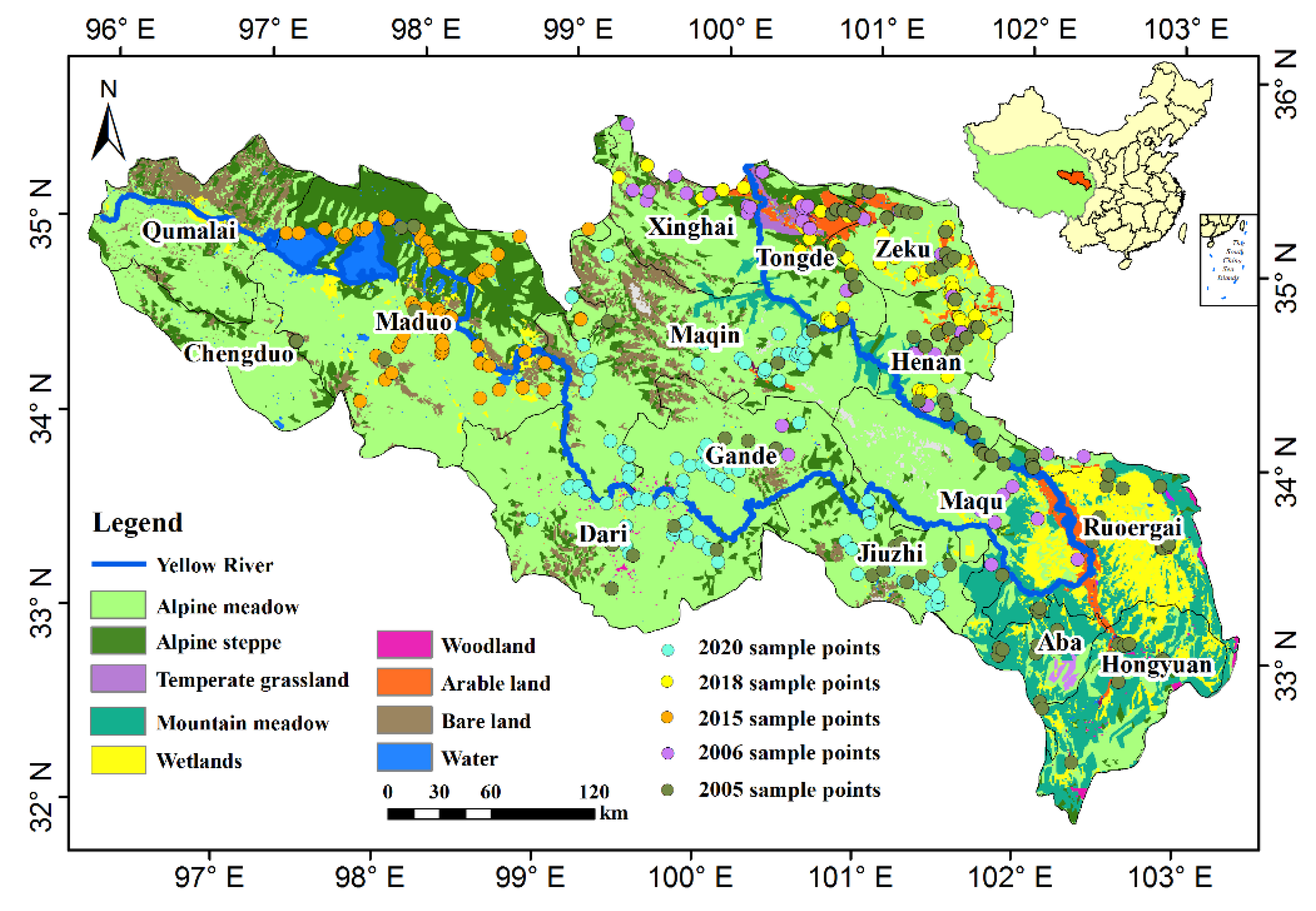
2.1. Study Area

The HYR is located at 32°30′–35°0′N, 95°50′–103°30′E (Figure 1), covering an area of approximately 12.37 × 10⁴ km2 [17], with an elevation between 2680–6248 m. The roads are rugged and few, and the average temperature for many years was concentrated between −12.7 °C and 5.6 °C (Figure 2a). The average rainfall from 2001 to 2020 was 579.50 mm, and the rainfall decreased from southeast to northwest. (Figure 2b), mainly concentrated in June to September, accounting for 90% of the total annual rainfall. Grassland is an important land cover type. Alpine meadows account for 61.40% of the entire study area; followed by alpine steppes (12.04%), mountain meadows (9.29%), wetlands (6.56%), bare land (5.52%), and arable land (2.11%); other land use types account for less than 1.0% (Figure 1). The main characteristics of the soil are thin soil layer, coarse soil quality, more gravel, and coarse sand in the soil (14.50% clay, 39.90% powder, and 38.17% sand) (Figure 2j–l); animal husbandry is the main activity.

2.2. Data Source and Preprocessing

2.2.1. AGB Data Source

We use the conditional Latin hypercube sampling (cLHS) method [18], which is restricted by the cost layer, to arrange the sampling points as evenly as possible in the HYR. The restricted variables, when using cLHS to lay out sample points, include meteorological data (such as rainfall and temperature), topographic data (such as elevation and slope), and soil data (such as powder and sand); the above variables are uniformly resampled to a spatial resolution of 500 m [18,19].
Road, elevation, and slope were considered the main environmental factors limiting the sample collection; weights of 0.5, 0.3, and 0.2 were assigned to the three variables, respectively, and cost layers were generated (Figure A1). The cost layers were created using ArcGIS software, and the cLHS sample points were laid out in R Studio software using the data package cLHS. The aboveground biomass data were collected in the growing seasons (July–August) in 2005, 2006, 2015, 2018, and 2020; one or two 0.5 × 0.5 m sample boxes were set up in sample plots with good vegetation community consistency, and three or four 0.5 × 0.5 m sample boxes were averaged in areas with more complex and uneven vegetation distribution. Samples were selected to represent, as much as possible, the vegetation growth of the whole area; all its aboveground biomass was collected, including apoplastic material. The samples were dried in the laboratory at 65 °C for 48 h to a constant weight and the dry weight was determined, resulting in a total of 501 measured aboveground biomass data.

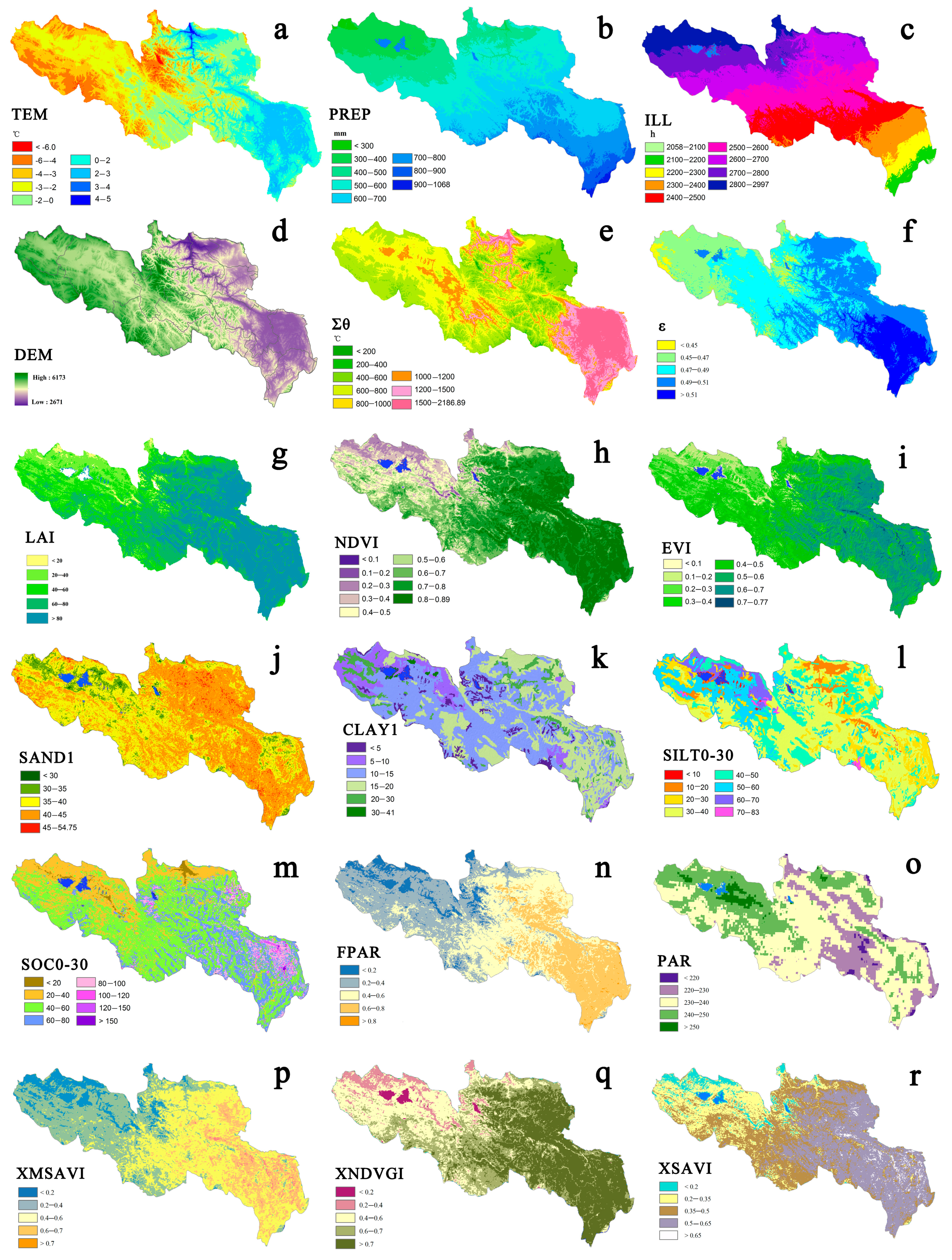
2.2.2. Environmental Variable Data Source

Environmental data parameters considered in this study are described in Table 1. The meteorological data comes from the spatial interpolation data calculated by our team. First, we downloaded the daily temperature, daily precipitation, daily wind speed, sunlight, longitude, latitude, and elevation data of 836 weather stations across the country, from 2001 to 2020 (http://data.cma.cn, accessed on 18 February 2021) (Figure A2). Then, the daily value data are calculated as monthly value data, according to the longitude, latitude, and altitude of each weather station; the weather station point data was interpolated into raster data, with a spatial resolution of 1 km, using ANUSPLIN software [20]. THE NDVI, EVI, and LAI were obtained from MODIS data products, and the data were downloaded through Google Earth Engine (https://code.earthengine.google.com/, GEE, accessed on 27 January 2021). The soil-related data were obtained from the Harmonized World Soil Database (HWSD) (https://data.isric.org/, accessed on 13 January 2021). The ε, PAR, and FPAR data were calculated using Zhu Wenquan’s improved CASA model [21]. All raster images in this paper use Krasovsky 1940 Albers projection. The main environmental variable factors are shown in Figure 2. According to the division of environmental variables in the STEP-AWBH model, the environmental variables collected in this study were included in four categories (Table 1): soil physical and chemical factors (S), topographic factors (T), meteorological factors (A), and vegetation factors (B).

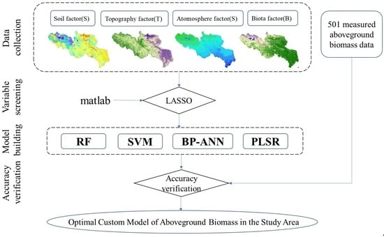
2.3. Methods and Modelling

2.3.1. Variable Selection

LASSO is a variable screening method with the advantage of statistical accuracy of variable selection and its computational feasibility. LASSO has the ability to handle multicollinearity data, by automatically selecting the most important independent variables and narrowing down the less important predictor variables to zero, so as to retain only the useful features [22].

2.3.2. Modeling Methods

The four modeling methods include partial least squares regression (PLSR), support vector machines (SVM), RF, and back-propagation artificial neural network (BP-ANN). PLSR is an extension of multiple linear regression. Compared with ordinary least squares regression, PLSR calculations are more reliable [23,24]. SVM was originally used for classification and has been widely used to solve the classification and regression problems of nonlinear and high-dimensional data [25]. In this paper, the radial basis function was used as the kernel function and the genetic algorithm was used to optimize two key parameters (gamma and cost) [26]. The most important parameters in the BP-ANN model are the number of neurons and hidden layers, which need to be repeatedly tested and continuously tuned [27]. RF is a machine learning algorithm that trains classification samples through decision trees and makes predictions based on the results of the classification [28]. The two most important parameters in the RF algorithm are the number of regression trees and the number of predictors at each node [29], which need to be optimized [3]. All machine learning models in this paper were trained, parameter tuned, and simulated in the Matlab 2017a software.

2.3.3. Model Accuracy Evaluation

Five-fold cross validation was used to evaluate the predictive performance of the model results. The coefficient of determination of the training dataset (R2train), root mean square error of the training dataset (RMSEtrain), R2 of the validation dataset (R2val), and the validation dataset RMSE (RMSEval) were used to evaluate the predictive ability of each model.

2.3.4. Trend Analysis

The Theil-Sen (SEN) median trend analysis and Mann-Kendall test were used to determine the significance of the trend of AGB [30,31]. When SENslope > 0, it reflected an increasing trend, and there was a decreasing trend for when the opposite was true (SENslope < 0). The significance of the changing trend of AGB was tested at the confidence level α = 0.05 (Table 2). When Z > |1.96| means confidence level α < 0.05, the change trend was significant, Z < |1.96| means confidence level α > 0.05, the change trend was not significant [32].

3. Results

3.1. Analysis of Model Results

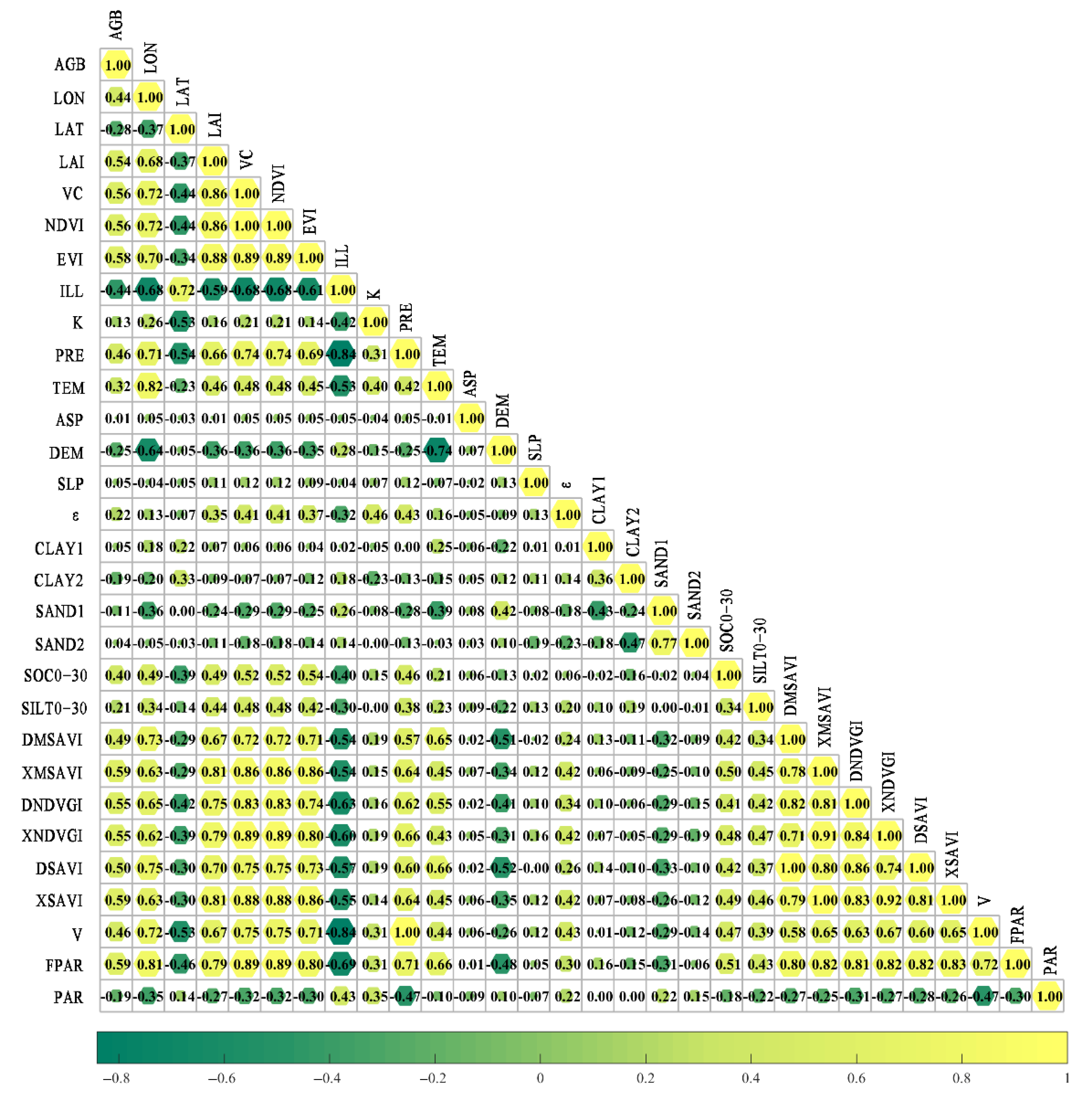
3.1.1. Correlation Analysis between AGB and Environmental Variables

The minimum value of all samples was 6.5 g/m2 (located in Maduo County) and the maximum value was 428.02 g/m2 (located in Hongyuan County). The average value of all samples was 171.39 g/m2. Overall, the average value of all samples decreased from the southeast to the northwest, and the county with the largest average value was Hongyuan County (with 292.59 g/m2), and the county with the smallest average value was Maduo County (with 102.02 g/m2) (Table 3).

3.1.2. Correlation Analysis between AGB and Environmental Variables

The correlation matrix represents the environmental variables and AGB, shown by the correlation coefficient (Figure 3). Positive correlations are shown in yellow, and negative correlations are shown in green. Among them, FPAR, XMSAVI, and XSAVI had the highest correlation with AGB (R = 0.59), except that there was a good correlation between various vegetation indices and the measured AGB; the correlations were all greater than 0.5, indicating that the vegetation index can better characterize the grassland in the HYR. Among the geographic location factors, longitude (R = 0.44) was more correlated with AGB than latitude (R = −0.28), elevation (R = −0.25), and slope (R = 0.05). Among the meteorological factors, annual rainfall (R = 0.46) and illumination (R = −0.44) better responded to the information of AGB, compared to mean annual TEM (R = 0.32) and K (R = 0.13). Among the soil factors, the correlation between SOC and AGB was significantly higher than that between CLAY and SAND. In addition, there were also strong correlations among the environmental variables; for example, the correlation coefficient between NDVI and coverage was 1, while the correlation between NDVI and EVI also reached 0.89. Therefore, if all variables are included in the machine learning algorithm for simulation, it will lead to the generation of the multicollinearity problem. Based on this problem, we did variable screening to determine the best input feature set, which is crucial to reduce model overfitting and improve model performance.

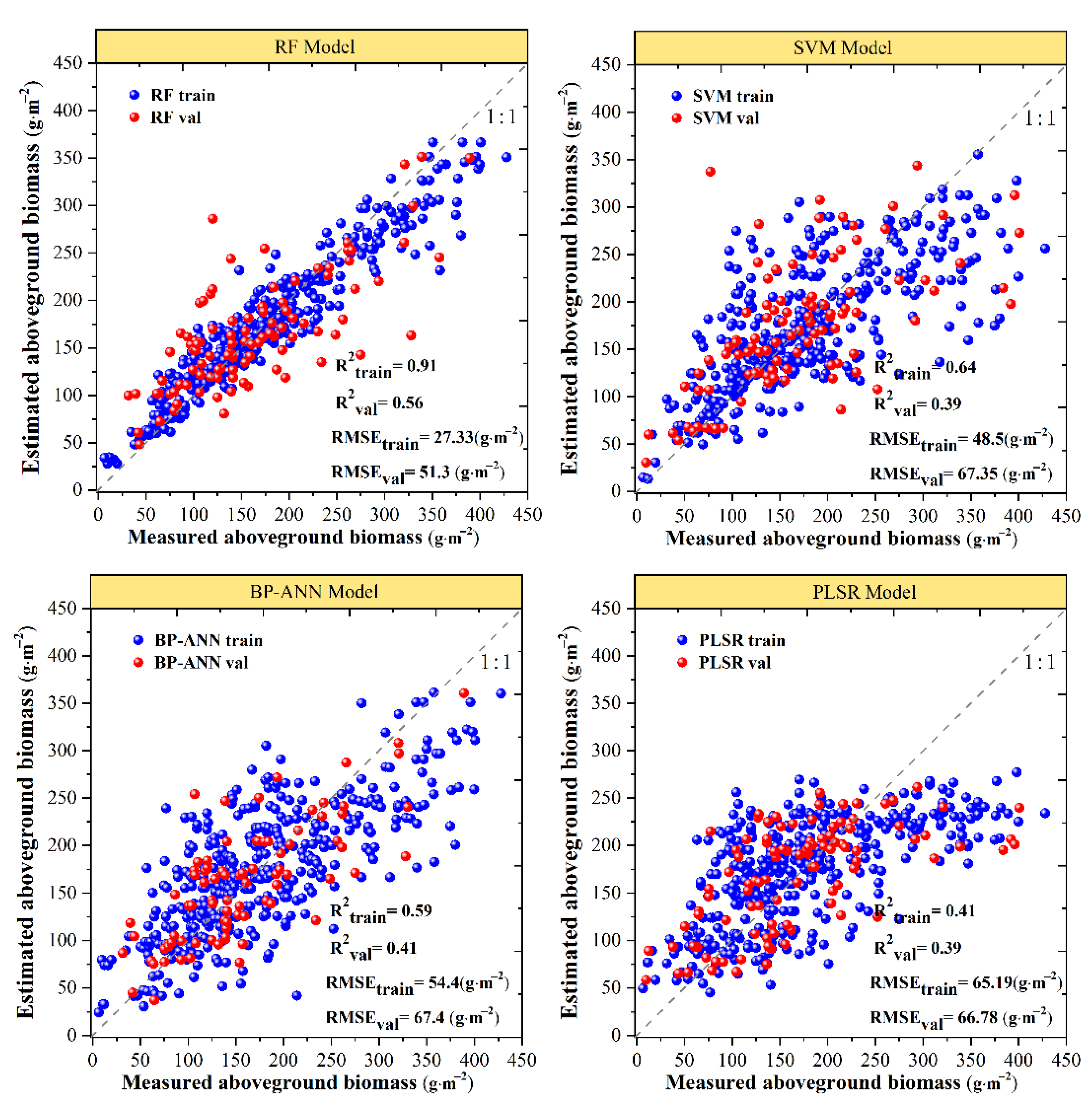
3.1.3. Model Accuracy Evaluation

LASSO selected 8 environmental variables. Longitude was selected in the geographic location factor, EVI, XMSAVI, and XNDVGI were selected in the vegetation index factor, illumination was selected in the meteorological factor, and CLAY2 and SOC were selected in the soil factor. In the CASA model, the FPAR variable was also selected. In the validation set of the four grassland AGB estimation models (Figure 4), RF had the highest R2val and lowest RMSEval of 0.56 and 51.3 g/m2, respectively. The second was BP-ANN, which were 0.41 and 67.4 g/m2, respectively. The R2val of SVM and PLSR were both 0.39, and the RMSEval was 67.35 g/m2 and 66.78 g/m2, respectively. The reason may be that (compared with models, such as BP-ANN and PLSR) the RF model introduces randomization to deal with the decision tree problem, which significantly improves the model’s resilience to noise [33,34]. Therefore, the RF method was used to estimate the AGB of the HYR from 2001 to 2020.

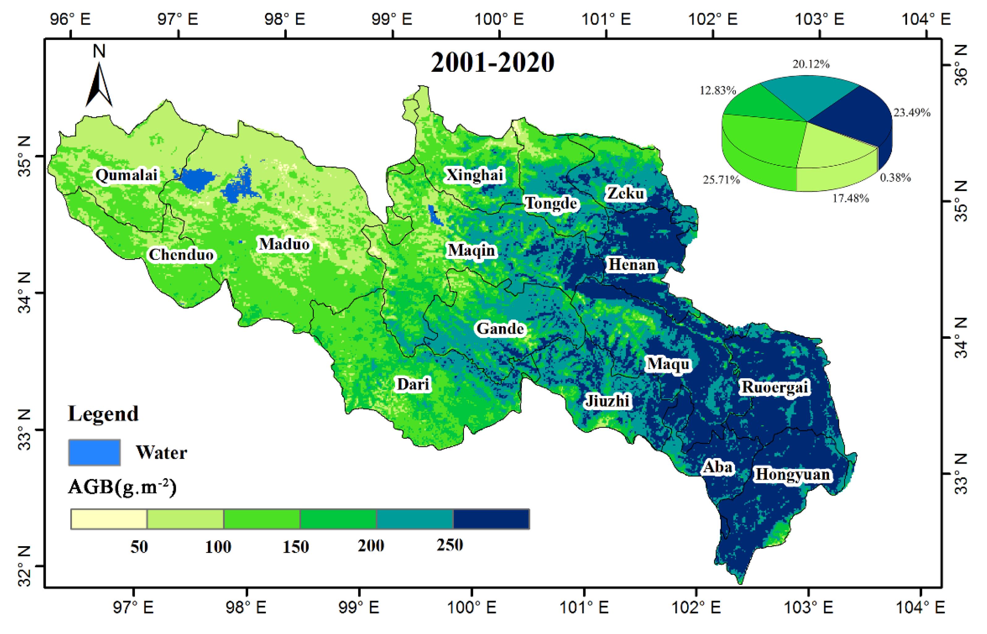
3.2. Spatial and Temporal Dynamic Distribution of AGB

In terms of spatial distribution, the spatial distribution of AGB in the HYR from 2001 to 2020 showed an obvious heterogeneity (Figure 5), showing a clear trend of gradual decline from southeast to northwest. The 2001–2020 AGB annual mean and AGB annual total values were 176.8 g/m2 and 20.73 Tg, respectively. The maximum biomass was 306 g/m2, mainly concentrated between 50–250 g/m2, accounting for 76.13%, distributed in Tongde, Zeku, Henan, Maqu, Jiuzhi, Gand, Dari, and MaQin counties. The percentage of those exceeding 250 g/m2 was 23.49% were distributed in Hongyuan, Aba, and Ruoerge counties. The smallest AGB values were distributed in Qumarai, Maduo, and Chengduo counties, in the northwestern region of the HYR. The average values from 2001 to 2020 were 82.46 g/m2, 98.23 g/m2, and 116.71 g/m2. The AGB values decreased spatially from southeast to northwest, and this trend was closely related to the rainfall, elevation, and vegetation distribution types in the region.

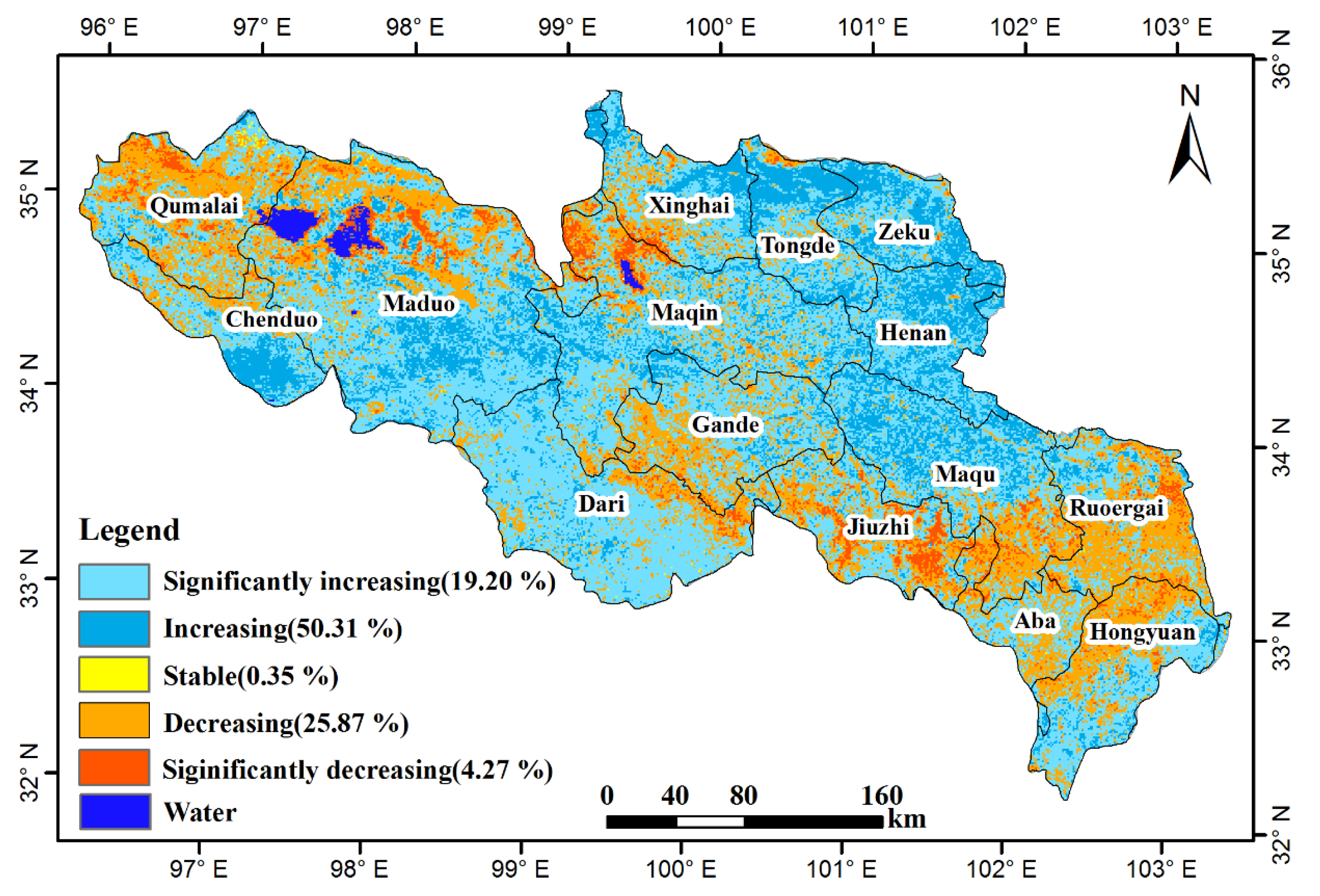
3.3. Trend Analysis of AGB Changes

The AGB in the HYR showed an increasing trend in most areas from 2001 to 2020, with 69.51% of the area increasing, 0.35% of the area remaining stable, and 30.14% of the area decreasing in AGB (Figure 6). Among them, the significantly increased areas accounted for 19.2%, mainly in the northern parts of Tongde, Zeku, Henan, and Maqu counties, as well as the southern parts of Maduo (Table 4). A total of 50.31% of the regional AGB showed a slight increase in trend, mainly distributed in Maqin and Dari counties. In addition, nearly 25.87% of the regional AGB showed a slight downward trend, mainly concentrated in northern Hongyuan county and southern Ruoerge, as well as southern Maqu, northern Quemalai, and Maduo counties. A significant decrease was observed in 4.27% of the areas, which were distributed in the southeastern part of Jiuzhi county, the northwestern part of Maqin, and the northern parts of Qumalai and Maduo counties (Figure 6).

4. Discussion

4.1. Compared with Traditional Univariate Model

The aboveground biomass in the HYR has a positive correlation with the remote sensing vegetation index (Table 5), indicating that it is basically feasible to use the vegetation index to monitor grassland biomass. Meanwhile, there were differences in the relationship between different vegetation indices and biomass, among which NDVI and AGB had the highest cubic correlation coefficient (R = 0.46); the curvilinear model better reflected the relationship between vegetation indices and measured biomass, compared to the univariate linear regression model. Overall, the correlation coefficient fit of NDVI and AGB was better than that of EVI, MSAVI, NDVGI, and SAVI. It shows that the use of NDVI cubic polynomial model is a simple, effective, and practical method to monitor AGB. Generally speaking, compared with the univariate model, RF improves the simulation accuracy of grassland AGB in the HYR, has higher stability, better predictive ability, strong application prospects, and advantages. Although the random forest model is significantly better than the traditional model, the custom model constructed in this study is only applicable to the HYR, for the time being. Whether it is applicable to other grassland types, such as cold desert, temperate grassland, and tropical grassland, remains to be further verified.

4.2. Reasons for AGB Changes

In the past 20 years, the vegetation status in the HYR has shown an overall improvement trend, which is consistent with existing research results [35,36,37]. Existing studies have shown that [38], affected by global warming, the HYR has generally shown a warm and humid trend in recent years, which provides favorable climatic conditions for vegetation restoration in the HYR. In this study, although temperature and rainfall were not screened as important environmental variables for simulating grassland AGB, the correlation coefficients of longitude with rainfall and temperature were 0.71 and 0.82, respectively; rainfall and temperature showed a gradual decrease from west to east, due to the geographical location of the Yellow River source area, so longitude better represented the climate influence factors in the region. The areas with the least AGB are located in Maduo County and the northern part of Chenduo County. The area is less affected by the southwest monsoon, has high altitude, poor water, and heat conditions, and therefore, poor vegetation growth. Lowering temperature will inhibit the growth and development of vegetation in this area, and rising temperature is conducive to the accumulation of dry matter quality of plants, which is a favorable condition for vegetation growth. This is the climatic factor of AGB decreasing from southeast to northwest in the HYR.
Human activities are equally important drivers of changes in grassland dynamics [39,40,41]. Since 2003, the region began to implement the policy of returning grazing to the grasslands. The purpose of the plan is to improve the grassland ecological environment, promote a virtuous cycle of grassland ecology, and maintain national ecological security. In 2011, the first phase of the ecological award policy was implemented in the region, and the second phase of the ecological award policy was started in 2016, which increased the amount of grass storage balance incentives and subsidies for grazing ban, compared to the first phase; in terms of policy ecological effects, the study showed that the ecological supplementation policy played a positive role in the ecological restoration and improvement of the Yellow River source area [42]. Thus, favorable policies may be the artificial reason why 69.51% of the regional AGB in the study area showed an increase. As the AGB in Zeku, Tongde, and Magu have shown an increasing trend in recent years (Figure 6), this is due to the fact that the area has adopted water and soil conservation prevention and protection projects and comprehensive desertification control projects, through fences, policy closures, water and soil conservation monitoring, and improvement of the legal system. It also carries out ecological restoration treatment of mines, power stations, and road construction projects, so that the regional ecological environment is significantly improved, and the cover of severely degraded areas is significantly increased [43]. On the other hand, areas of AGB degradation, occurring in this study, were mainly concentrated in Aba, Hongyuan, and Maduo counties; according to research by Xu et al. [44], there are overgrazing situations in Aba and Hongyuan, while the total number of livestock in Henan, Tongde, Xinghai, and Zeku counties has shown a downward trend. Therefore, the increase in grazing pressure will reduce the carrying capacity of the grassland, which will degrade the grassland. In degraded areas of AGB, since animal husbandry is the main source of income for local herders, it is obviously unrealistic to implement large-scale grazing prohibitions. We should graze scientifically, determine animals with grass, manage scientifically, use grassland rationally, and restore natural grassland productivity [45], focus on the construction of pasture fences, determine a reasonable pasture carrying capacity, scientifically configure the herd structure, implement zoning and grazing in turns, so that natural pastures can be recuperated, and develop grassland irrigation and fertilization in areas where conditions permit, and improve natural pastures [46].

4.3. Advantages and Limitations of Custom Models

First, the machine learning algorithm can incorporate a variety of environmental variables that affect AGB into the model simulation study. In addition, the input variable data are easy to obtain, and the model can independently learn and adjust parameters, which has strong applicability. The model can be adapted to the study of different research areas, and even with the support of sufficiently complete data, the prediction range can be further improved. Although our research provides a comprehensive assessment of the AGB in the HYR, there are still some limitations. First, due to inconvenient transportation, there are relatively few sampling points in the western region; this may result in inaccurate AGB estimates for the region. Secondly, as a black box operation, the learning process of a machine learning model is uncontrollable. Third, when the random forest is performing regression, it cannot make predictions that exceed the range of the training set data; it does not perform as well in classification, because it cannot give a continuous output [47].

5. Conclusions

The simulation results of the RF algorithm are better than the SVM, BP-ANN, PLSR, and univariate vegetation index model (R2val = 0.56, RMSEval = 51.3 g/m2). From 2001 to 2020, the AGB of the HYR showed a spatially decreasing trend from the southeast to northwest, and the proportion of the area with increasing grassland AGB reached 69.51% in the past 20 years, while the proportion of the area with decreasing grassland AGB was 30.14%, mainly in Hongyuan, Ruoerge, Jiuzhi, and Qumalai counties. This study has a high sampling site density and small model deviation, which accurately simulates the spatial distribution pattern of soil erosion in the HYR. The research results can not only provide a scientific basis for the grassland management and protection policies in the HYR, but also extend the application of such modeling methods to the study of grassland AGB in other areas of the Qinghai-Tibet Plateau.

Author Contributions

Conceptualization, H.L. and R.T.; methodology, R.T. and Y.Z.; software, R.T. and Y.Z.; validation, R.T. and Y.Z.; formal analysis, R.T.; investigation, R.T. and Y.Z.; resources, R.T. and Y.Z.; data curation, H.L.; writing—original draft preparation, R.T.; writing—review and editing, R.T. and Y.Z.; visualization, R.T. and Y.Z.; supervision, H.L.; project administration, H.L.; funding acquisition, H.L. All authors have read and agreed to the published version of the manuscript.

Funding

This work was supported by the National Natural Science Foundation of China (32171680 and 31772666), and the Fundamental Research Funds for the Central Universities (lzujbky-2021-kb13).

Institutional Review Board Statement

Not applicable.

Informed Consent Statement

Not applicable.

Data Availability Statement

Not applicable.

Acknowledgments

We are very grateful for the constructive comments provided by the three anonymous reviewers and academic editor, who gave us a huge help during the article publication process.

Conflicts of Interest

The authors declare no conflict of interest.

Appendix A

In Figure A1, we showed the cost map of using the cLHS method to lay out the sample points, thus laying the foundation for the scientific collection of samples to make belts. In Figure A2, we showed the distribution of meteorological stations, which is the basis for all meteorological data in this paper.
Figure A1. Cost layer obtained with cLHS.
Remotesensing 13 03404 g0a1
Figure A2. Weather station distribution map.
Remotesensing 13 03404 g0a2

References

  1. White, R.P.; Murray, S.; Rohweder, M.; White, R.P.; Murray, S.; Rohweder, M. Pilot analysis of global ecosystems: Grassland ecosystems. World Resour. Inst. 2000, 4, 275. [Google Scholar]
  2. Curlock, J.M.O.S.; Hall, D.O. The global carbon sink: A grassland perspective. Glob. Chang. Biol. 2010, 4, 229–233. [Google Scholar] [CrossRef] [Green Version]
  3. Gao, X.X.; Dong, S.K.; Li, S.; Xu, Y.D.; Liu, S.L.; Zhao, H.D.; Yeomans, J.; Li, Y.; Shen, H.; Wu, S.N.; et al. Using the random forest model and validated MODIS with the field spectrometer measurement promote the accuracy of estimating aboveground biomass and coverage of alpine grasslands on the Qinghai-Tibetan Plateau. Ecol. Indic. 2020, 112, 106114. [Google Scholar] [CrossRef]
  4. Zeng, N.; Ren, X.; He, H.; Zhang, L.; Zhao, D.; Ge, R.; Li, P.; Niu, Z. Estimating grassland aboveground biomass on the Tibetan Plateau using a random forest algorithm. Ecol. Indic. 2019, 102, 479–487. [Google Scholar] [CrossRef]
  5. Zhou, W.; Li, H.R.; Xie, L.; Nie, X.; Wang, Z.; Du, Z.; Yue, T. Remote sensing inversion of grassland aboveground biomass based on high accuracy surface modeling. Ecol. Indic. 2021, 121, 107215. [Google Scholar] [CrossRef]
  6. Zhang, J.; Zhang, L.; Liu, W.; Qi, Y.; Wo, X. Livestock-carrying capacity and overgrazing status of alpine grassland in the Three-River Headwaters region, China. J. Geogr. Sci. 2014, 24, 303–312. [Google Scholar] [CrossRef]
  7. Xu, B.; Yang, X.C.; Tao, W.G.; Qin, Z.H.; Liu, H.Q.; Miao, J.M. MODIS-based remote sensing monitoring of grass production in China. Int. J. Remote Sens. 2008, 29, 5313–5327. [Google Scholar] [CrossRef]
  8. Diallo, O.; Ddiouf, A.; Hanan, N.P.; Ndiaye, A.; Prevost, Y. AVHRR monitoring of savanna primary production in Senegal, West Africa: 1987–1988. Int. J. Remote Sens. 1991, 12, 1259–1279. [Google Scholar] [CrossRef]
  9. Nouri, H.; Anderson, S.; Sutton, P.; Beecham, S.; Nagler, P.; Jarchow, C.J.; Roberts, D.A. NDVI, scale invariance and the modifiable areal unit problem: An assessment of vegetation in the Adelaide Parklands. Sci. Total Environ. 2017, 584–585, 11–18. [Google Scholar] [CrossRef]
  10. Paruelo, J.M.; Epstein, H.E.; Lauenroth, W.K.; Burke, I.C. ANPP estimates from NDVI for the central grassland region of the US. Ecology 1997, 78, 953–958. [Google Scholar] [CrossRef]
  11. Idowu, S.; Saguna, S.; Ahlund, C.; Schelen, O. Applied Machine Learning: Forecasting Heat Load in District Heating System. Energy Build. 2016, 133, 478–488. [Google Scholar] [CrossRef]
  12. Wang, Y.; Wu, G.; Lei, D.; Tang, Z.; Shangguan, Z. Prediction of aboveground grassland biomass on the Loess Plateau, China, using a random forest algorithm. Sci. Rep. 2017, 7, 6940. [Google Scholar] [CrossRef] [Green Version]
  13. Xie, Y.; Sha, Z.; Yu, M.; Bai, Y.; Zhang, L. A comparison of two models with Landsat data for estimating above ground grassland biomass in Inner Mongolia, China. Ecol. Model. 2009, 220, 1810–1818. [Google Scholar] [CrossRef]
  14. Yang, S.X.; Feng, Q.S.; Liang, T.G.; Liu, B.; Zhang, W.; Xie, H. Modeling grassland above-ground biomass based on artificial neural network and remote sensing in the Three-River Headwaters Region. Remote Sens. Environ. 2017, 204, 448–455. [Google Scholar] [CrossRef]
  15. Chu, H.; Wei, J.; Li, T.; Jia, K. Application of Support Vector Regression for Mid- and Long-term Runoff Forecasting in “Yellow River Headwater” Region. Procedia Eng. 2016, 154, 1251–1257. [Google Scholar] [CrossRef] [Green Version]
  16. Yang, L.; Li, X.; Shi, J.; Shen, F.; Zhou, C.J.G. Evaluation of conditioned Latin hypercube sampling for soil mapping based on a machine learning method. Geoderma 2020, 369, 114337. [Google Scholar] [CrossRef]
  17. Luo, D.; Jin, H.; Bense, V.F.; Jin, X.; Li, X. Hydrothermal processes of near-surface warm permafrost in response to strong precipitation events in the Headwater Area of the Yellow River, Tibetan Plateau. Geoderma 2020, 376, 114531. [Google Scholar] [CrossRef]
  18. Ma, T.; Brus, D.J.; Zhu, A.X.; Zhang, L.; Scholten, T.J.G. Comparison of conditioned Latin hypercube and feature space coverage sampling for predicting soil classes using simulation from soil maps. Geoderma 2020, 370, 114366. [Google Scholar] [CrossRef]
  19. McBratney, M. A conditioned Latin hypercube method for sampling in the presence of ancillary information. Comput. Geosci. 2006, 32, 1378–1388. [Google Scholar]
  20. Wang, C.; Lin, H.L.; Zhao, Y.T. A Modification of CIM for Prediction of Net Primary Productivity of the Three-River Headwaters, China. Rangel. Ecol. Manag. 2019, 72, 327–335. [Google Scholar] [CrossRef]
  21. Zhu, W.Q.; Pan, Y.Z.; Zhang, J.S. Estimation of Net Primary Productivity of Chinese Terrestrial Vegetation Based on Remote Sensing. J. Plant Ecol. 2007, 31, 413–424. [Google Scholar]
  22. Niharika, G. Introduction to the LASSO. Resonance 2018, 23, 439–464. [Google Scholar]
  23. Li, D.; Chen, Y. Computer and Computing Technologies in Agriculture V. Comput. Comput. Technol. Agric. 2016, 295, 104–112. [Google Scholar]
  24. Yang, X.; Liu, G.; He, J.; Kang, N.; Yuan, R.; Fan, N. Determination of sugar content in Lingwu jujube by NIR–hyperspectral imaging. J. Food Sci. 2021, 86, 1201–1214. [Google Scholar] [CrossRef] [PubMed]
  25. Ge, J.; Meng, B.P.; Liang, T.G.; Feng, Q.S.; Gao, J.L.; Yang, S.X.; Huang, X.D.; Xie, H. Modeling alpine grassland cover based on MODIS data and support vector machine regression in the headwater region of the Huanghe River, China. Remote Sens. Environ. 2018, 218, 162–173. [Google Scholar] [CrossRef]
  26. Gao, J.; Meng, B.; Liang, T.; Feng, Q.; Ge, J.; Yin, J.; Wu, C.; Cui, X.; Hou, M.; Liu, J.J.; et al. Modeling alpine grassland forage phosphorus based on hyperspectral remote sensing and a multi-factor machine learning algorithm in the east of Tibetan Plateau, China. ISPRS J. Photogramm. Remote Sens. 2019, 147, 104–117. [Google Scholar] [CrossRef]
  27. Xin, L.; Li, X.B.; Gong, J.R.; Li, S.K.; Wang, H.S.; Dang, D.L.; Xuan, X.J.; Wang, H. Remote-sensing inversion method for aboveground biomass of typical steppe in Inner Mongolia, China. Ecol. Indic. 2020, 120, 106683. [Google Scholar]
  28. Breiman, L. Random Forests. Mach. Learn. 2001, 45, 5–32. [Google Scholar] [CrossRef] [Green Version]
  29. Li, W.; Zhou, X.; Zhu, X.; Dong, Z.; Guo, W. Estimation of biomass in wheat using random forest regression algorithm and remote sensing data. Crop J. 2016, 3, 62–69. [Google Scholar]
  30. Ullah, S.; You, Q.; Ali, A.; Ullah, W.; Xie, X. Observed changes in maximum and minimum temperatures over China- Pakistan economic corridor during 1980–2016. Atmos. Res. 2019, 216, 37–51. [Google Scholar] [CrossRef]
  31. Wang, Y.; Huang, X.; Hui, L.; Sun, Y.; Feng, Q.; Liang, T.J. Tracking Snow Variations in the Northern Hemisphere Using Multi-Source Remote Sensing Data (2000–2015). Remote Sens. 2018, 10, 136. [Google Scholar] [CrossRef] [Green Version]
  32. Yin, S.; Guo, M.; Wang, X.; Yamamoto, H.; Ou, W. Spatiotemporal variation and distribution characteristics of crop residue burning in China from 2001 to 2018. Environ. Pollut. 2020, 268, 115849. [Google Scholar] [CrossRef] [PubMed]
  33. Ao, Y.; Li, H.Q.; Zhu, L.P.; Ali, S.; Yang, Z.G. The linear random forest algorithm and its advantages in machine learning assisted logging regression modeling. J. Pet. Sci. Eng. 2019, 174, 776–789. [Google Scholar] [CrossRef]
  34. Vincenzi, S.; Zucchetta, M.; Franzoi, P.; Pellizzato, M.; Pranovi, F.; De Leo, G.A.; Torricelli, P. Application of a Random Forest algorithm to predict spatial distribution of the potential yield of Ruditapes philippinarum in the Venice lagoon, Italy. Ecol. Model. 2011, 222, 1471–1478. [Google Scholar] [CrossRef]
  35. Yang, Z.P.; Gao, J.X.; Zhou, C.P.; Shi, P.L.; Zhao, L.; Shen, W.S.; Ouyang, H. Spatio-temporal changes of NDVI and its relation with climatic variables in the source regions of the Yangtze and Yellow rivers. J. Geogr. Sci. 2011, 21, 979–993. [Google Scholar] [CrossRef]
  36. Guo, B.; Zang, W.Q.; Yang, F.; Han, B.M.; Chen, S.T.; Liu, Y.; Yang, X.; He, T.L.; Chen, X.; Liu, C.T.; et al. Spatial and temporal change patterns of net primary productivity and its response to climate change in the Qinghai-Tibet Plateau of China from 2000 to 2015. J. Arid Land 2020, 12, 1–17. [Google Scholar] [CrossRef] [Green Version]
  37. Xiong, Q.L.; Xiao, Y.; Halmy, M.W.A.; Dakhil, M.A.; Liang, P.H.; Liu, C.G.; Zhang, L.; Pandey, B.; Pan, K.W.; El Kafraway, S.B.; et al. Monitoring the impact of climate change and human activities on grassland vegetation dynamics in the northeastern Qinghai-Tibet Plateau of China during 2000–2015. J. Arid Land 2019, 11, 637–651. [Google Scholar] [CrossRef] [Green Version]
  38. Tian, H.; Lan, Y.C.; Wen, J.; Jin, H.J.; Wang, C.H.; Wang, X.; Kang, Y. Evidence for a recent warming and wetting in the source area of the Yellow River (SAYR) and its hydrological impacts. J. Geogr. Sci. 2015, 25, 643–668. [Google Scholar] [CrossRef]
  39. Cai, H.Y.; Yang, X.H.; Xu, X.L. Human-induced grassland degradation/restoration in the central Tibetan Plateau: The effects of ecological protection and restoration projects. Ecol. Eng. J. Ecotechnol. 2015, 83, 112–119. [Google Scholar] [CrossRef]
  40. Liu, Y.Y.; Wang, Q.; Zhang, Z.Y.; Tong, L.J.; Wang, Z.Q.; Li, J.L. Grassland dynamics in responses to climate variation and human activities in China from 2000 to 2013. Sci. Total Environ. 2019, 690, 27–39. [Google Scholar] [CrossRef]
  41. Yang, Y.; Wang, Z.Q.; Li, J.L.; Gang, C.C.; Zhang, Y.Z.; Zhang, Y.; Odeh, I.; Qi, J.G. Comparative assessment of grassland degradation dynamics in response to climate variation and human activities in China, Mongolia, Pakistan and Uzbekistan from 2000 to 2013. J. Arid Environ. 2016, 135, 164–172. [Google Scholar] [CrossRef]
  42. Wu, Y.; Wu, T.M.; Lin, H.L. elevation on the effect of the grassland ecological compensation policy on livestock reduction in the yellow river source area. Chin. J. Grassl. 2020, 42, 137–144. [Google Scholar]
  43. Yin, B.K.; Cao, X.Y.; Zhang, J.G.; Zhang, D.; Wang, X.Y. soil and water loss change in source region of the yellow river during 1999–2018. Bull. Soil Water Conserv. 2020, 40, 216–220. [Google Scholar]
  44. Xu, H.J.; Wang, X.P.; Zhang, X.X. Impacts of climate change and human activities on the aboveground production in alpine grasslands: A case study of the source region of the Yellow River, China. Arab. J. Geosci. 2017, 10, 1–14. [Google Scholar] [CrossRef]
  45. Feng, J.M.; Tao, W.; Xie, C.W. Eco-Environmental Degradation in the Source Region of the Yellow River, Northeast Qinghai-Xizang Plateau. Environ. Monit. Assess. 2006, 122, 125–143. [Google Scholar] [CrossRef] [PubMed]
  46. Liu, Q.G.; Chen, X.P. Land-Cover Changes’ Mechanism and Some Proposals in the Source Regions of the Yellow River from Remote Sensing Date and GIS Technique. Ecol. Econ. 2009, 12, 54–59. [Google Scholar]
  47. Meyer, H.; Lehnert, L.W.; Wang, Y.; Reudenbach, C.; Nauss, T.; Bendix, J. From local spectral measurements to maps of vegetation cover and biomass on the Qinghai-Tibet-Plateau: Do we need hyperspectral information? Int. J. Appl. Earth Obs. Geoinf. 2017, 55, 21–31. [Google Scholar] [CrossRef]
Figure 1. Study area and sample points.
Remotesensing 13 03404 g001
Figure 2. Spatial distribution of main environmental variables (The information of Figure (a)–(r) is shown in Table 1).
Remotesensing 13 03404 g002
Figure 3. Correlation between AGB and various environmental variables.
Remotesensing 13 03404 g003
Figure 4. Accuracy evaluation of AGB simulated by different simulation methods.
Remotesensing 13 03404 g004
Figure 5. Spatial distribution of AGB in the HYR (the pie chart shows the proportion of AGB distribution ranges).
Remotesensing 13 03404 g005
Figure 6. The trend of AGB Change in the HYR from 2001 to 2020.
Remotesensing 13 03404 g006
Table 1. All environment variables and data sources.
CategoryAbbreviationVariable InterpretationResolutionData Sources
SCLAY1Clay content (0–30 cm)250 mHWSD
SCLAY2Clay content (30–100 cm)250 mHWSD
SSAND1Sand content (0–30 cm)250 mHWSD
SSAND2Sand content (30–100 cm)250 mHWSD
SSILT0-30Silt content (0–30 cm)250 mHWSD
SSOC0-30Soil organic carbon (0–30 cm)250 mHWSD
APREPAnnual temperature (2001–2020)1000 mMeteorological Station
ATEMAnnual precipitation (2001–2020)1000 mMeteorological Station
AKHumidity (2001–2020)1000 mMeteorological Station
AΣθ≥0 °C Annual cumulative temperature (2001–2020)1000 mMeteorological Station
AVActual evapotranspiration (2001–2020)1000 mMeteorological Station
AILLIllumination time (2001–2020)1000 mMeteorological Station
TDEMElevation30 mSRTM
TSLPSlope30 mArcGIS Calculated
TASPAspect30 mArcGIS Calculated
TLONLongitude30 mArcGIS Calculated
TLATLatitude30 mArcGIS Calculated
BEVIEnhanced vegetation index (2001–2020)1000 mMOD13A2
BNDVINormalized difference vegetation index (2001–2020)1000 mMOD13Q1
BVCVegetation cover (2001–2020)1000 mDimidiate Pixel Model
BLAILeaf area index (2001–2020)1000 mMOD15A2
BDMSAVIWinter modified soil adjusted vegetation index (2001–2020)1000 mMOD09A1 Band Calculated
BXMSAVISummer modified soil adjusted vegetation index (2001–2020)1000 mMOD09A1 Band Calculated
BDNDVGIWinter normalized difference vegetation green index (2001–2020)1000 mMOD09A1 Band Calculated
BXNDVGISummer normalized difference vegetation green index (2001–2020)1000 mMOD09A1 Band Calculated
BDSAVIWinter soil adjusted vegetation green index (2001–2020)1000 mMOD09A1 Band Calculated
BXSAVISummer soil adjusted vegetation green index (2001–2020)1000 mMOD09A1 Band Calculated
BPARPhotosynthetically active radiation (2001–2020)1000 mBESS PAR
BFPARFraction of photosynthetically active radiation (2001–2020)1000 mCASA
BεActual light use efficiency (2001–2020)1000 mCASA
Table 2. Aboveground biomass change trend assessment table.
SENslopeZTrend
>0.001>1.96Significantly incresaing
>0.001−1.96–1.96Incresaing
−0.001–0.001−1.96–1.96Stable
<−0.001−1.96–1.96Decreasing
<−0.001<−1.96Significantly decreasing
Table 3. Summary statistics of measured AGB (g/m2).
CountyMinMaxAverageStandard Deviation
Xinghai44.00233.92104.3746.00
Maduo6.50252.44102.0253.62
Tongde34.47264.44119.2268.06
Zeku96.66321.36163.8750.79
Maqin11.00374.92167.1778.29
Henan143.88400.79265.1464.36
Gande100.34210.64146.3337.45
Maqu83.77328.30164.4863.13
Dari77.96220.00151.2135.77
Ruoergai63.00357.50191.1986.98
Jiuzhi74.92380.20188.0888.15
Aba86.40253.60164.1239.32
Hongyuan104.01428.02292.56101.10
Total6.50428.02171.3984.89
Table 4. The dynamic change trend of AGB in each county.
CountyObviously IncreaseSlightly IncreaseStableSlightly IncreasingObviously Decrease
Xinghai24.60%50.13%0.36%21.57%3.34%
Qumalai4.66%35.07%1.48%50.11%8.69%
Maduo21.31%51.25%0.40%22.42%4.62%
Tongde39.72%46.91%0.15%12.42%0.80%
Zeku49.08%45.35%0.09%5.27%0.21%
Maqin18.65%56.58%0.24%19.84%4.68%
Chengduo28.39%50.11%0.52%19.72%1.26%
Henan49.12%48.53%0.02%2.30%0.04%
Gande11.49%53.56%0.19%32.77%1.98%
Maqu30.95%45.11%0.08%20.52%3.34%
Dari7.76%74.06%0.28%16.07%1.83%
Ruoergai6.59%33.74%0.46%52.50%6.71%
Jiuzhi6.00%42.63%0.08%36.92%14.36%
Aba3.66%48.27%0.40%43.43%4.24%
Hongyuan9.02%47.18%0.24%38.76%4.80%
Table 5. Fitting results of vegetation index and AGB.
IndexModelFormulaR2
NDVILinear y = 0.0011x + 0.52940.313
Exponential y = 0.5031e0.0018x0.2758
Power y = 0.1375x0.32130.4041
Logarithmic y = 0.1788ln(x) − 0.18480.4313
Quadratic y = −6 × 10−6x2 + 0.0035x + 0.32780.4327
Cubic y = 3 × 108x3 − 2 × 105x2 + 0.0063x + 0.20230.4564
EVILinear y = 9.9831x + 3434.50.3307
Exponential y = 3247.5e0.0024x0.2885
Power y = 706.02x0.38590.3841
Logarithmic y = 1567.1ln(x) − 2692.50.3885
Quadratic y = −0.0456x2 + 28.372x + 1949.90.4068
Cubic y = 7 × 105x3 − 0.0867x2 + 35.423x + 1625.90.4087
XMSAVILinear y = 0.001x + 0.32810.3478
Exponential y = 0.3174e0.0023x0.3077
Power y = 0.0684x0.38710.3983
Logarithmic y = 0.1562ln(x) − 0.28130.4023
Quadratic y = −4 × 10−6x2 + 0.0027x + 0.19440.4121
Cubic y = 5 × 109x3 −7 × 10−6 x2 + 0.0032x + 0.16960.4133
XNDVGILinear y = 0.0007x + 0.55430.3001
Exponential y = 0.5448e0.0011x0.2809
Power y = 0.2551x0.18910.3877
Logarithmic y = 0.109ln(x) + 0.12130.3977
Quadratic y = −3 × 10−6x2 + 0.002x + 0.44380.3894
Cubic y = 108x3 − 105x2 + 0.0033x + 0.38290.4033
XSAVILinear y = 0.0009x + 0.34620.3426
Exponential y = 0.3352e0.002x0.3073
Power y = 0.0875 × 0.33760.402
Logarithmic y = 0.1356ln(x) − 0.18520.4089
Quadratic y = −4 × 10−6x2 + 0.0024x + 0.22510.4138
Cubic y = 7 × 109x3 − 8 × 10−6x2 + 0.0031x + 0.19120.4166
Publisher’s Note: MDPI stays neutral with regard to jurisdictional claims in published maps and institutional affiliations.

