Quantifying Floating Plastic Debris at Sea Using Vessel-Based Optical Data and Artificial Intelligence

Abstract

Despite recent advances in remote sensing of large accumulations of floating plastic debris, mainly in coastal regions, the quantification of individual macroplastic objects (>50 cm) remains challenging. Here, we have trained an object-detection algorithm by selecting and labeling footage of floating plastic debris recorded offshore with GPS-enabled action cameras aboard vessels of opportunity. Macroplastic numerical concentrations are estimated by combining the object detection solution with bulk processing of the optical data. Our results are consistent with macroplastic densities predicted by global plastic dispersal models, and reveal first insights into how camera recorded offshore macroplastic densities compare to micro- and mesoplastic concentrations collected with neuston trawls.

1. Introduction

Plastic waste is an increasing threat to the natural environment [1]. The yearly global production of plastics grows exponentially [2]. Mismanaged waste has a high probability of reaching the natural environment and hydrosphere [3]. Rivers can transport plastic litter to the coastal zones [3,4,5,6], where they are transported further by oceanic dispersal into accumulation zones, for example, the Great Pacific Garbage Patch (GPGP), together with plastic litter emitted directly at sea by activities such as fishing, aquaculture, and shipping [7,8,9,10]. There, repetitive quantification efforts remain relevant as the concentration of plastic litter in the oceans depicts a high spatio-temporal variability [11,12] and because quantities keep on increasing [10,13].

A proven method for micro- and mesoplastic (<5 cm) quantification is to deploy a Manta trawl at the ocean surface. Here, a small surface net is trawled behind a research vessel. Subsequently, numerical and mass concentrations of plastic are determined by counting and weighing the plastic pieces collected by the trawl within a known sampled ocean surface area. Another method, visual observation, focuses on macroplastic (>50 cm) [8,14,15,16,17,18]. Numerical concentrations are obtained by visual counting of floating plastic debris from a vessel during a specific time interval. Manta-trawling and visual surveys are reliable but also labor- and time-intensive methods, making large-scale and systematic surveying in remote areas difficult.

Remote sensing of (floating) plastic litter provides a promising new and less labor-intensive tool for the quantification and characterization of ocean plastic pollution. This relatively new approach has seen recent successful developments on several applications. For example, unmanned aerial vehicles (UAVs) or airplanes equipped with optical cameras have successfully been used to quantify litter on beaches [19,20,21,22,23]. The mapping of floating litter is further pioneered by photography from airplanes [10,24] or satellite detection of large accumulated patches [25,26,27,28,29,30]. Finally, there are several developments towards automatic recognition of floating litter from UAVs [31,32,33] or bridge cameras [34]. It is likely that all these methods can be enhanced by multispectral or hyperspectral sensing [35,36,37,38,39,40,41].

However, most of these previous remote sensing approaches either focused on detecting debris in controlled or stationary environments or on vast debris accumulations, usually composed of a mix of floating anthropogenic and organic waste and often related to extreme environmental events. Individual large macroplastic items (floating plastic objects such as crates, ghost nets, or buoys >50 cm) in offshore marine environments are sparsely distributed with only a few objects per km² of sea surface area in accumulation zones such as the oceanic subtropical gyres [10]. Still, they may represent a substantial part of the floating plastic mass budget in the ocean because of their weight compared to microplastics (<5 mm). Despite opportunistic efforts to map them in certain areas [24,42,43], macroplastics remain poorly quantified in remote oceanic environments.

Current knowledge on the accumulation of macroplastic debris at the ocean surface is limited mainly due to methodological constraints. Macroplastics are typically too large for collection by neuston trawls. Furthermore, the relatively small sea surface area investigated during offshore research expeditions often is too small to compensate for the low areal concentrations of macroplastic debris. Given their contribution to floating plastic mass in the ocean [10], an accurate mass balance budget requires quantitative data on the distribution of macroplastics afloat on the sea surface.

Theoretically, the aforementioned visual observation method can be used to further quantify floating macroplastic debris, but a more scalable, standardized, and automated approach would be desirable for practical reasons. Here, we present a proof-of-concept for an alternative method, based on automatic object detection and analysis in camera transect images. In the method, we describe how GoPro^® action cameras were used to collect geo-tagged images. This is followed by the training and testing of a neural network and further geometric projections of the data. Finally, we describe the spatial aggregation of the camera-based observations and its comparison with observations of other size classes derived by concurrent Manta trawling.

2. Materials and Methods

2.1. 2019. Expedition Data

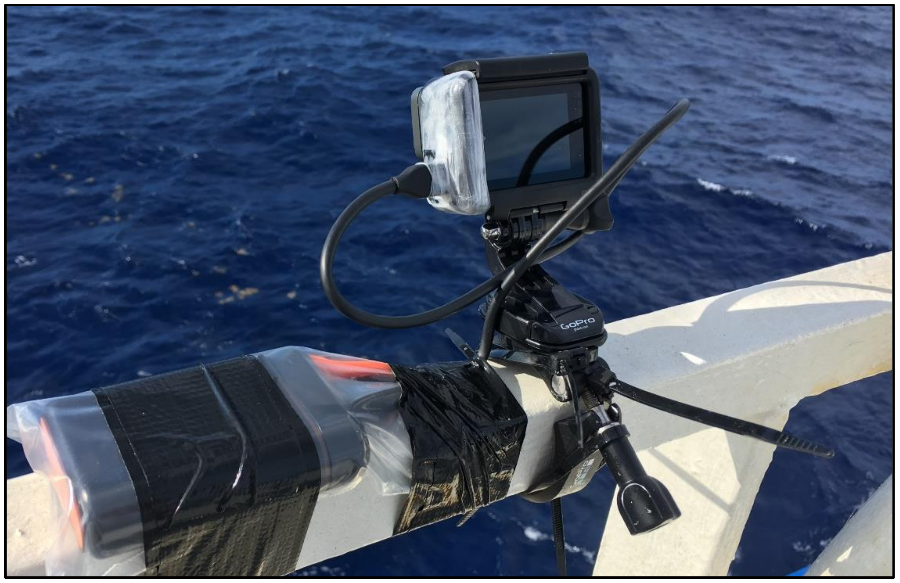
In late 2019, The Ocean Cleanup North Pacific Mission 3 (NPM3) took place aboard the Maersk Transporter [13]. GoPro^® cameras, Figure 1, mounted on starboard and portside at the bridge deck (18 m above the waterline) of the vessel traveling at 10 knots, recorded over 300,000 photos along transects during daytime conditions. As Figure 2 shows, this resulted in a data footprint that spans the area between the port of departure and arrival (Vancouver) and the area of interest, the Great Pacific Garbage Patch (GPGP). The cameras recorded photo time-lapses with intervals varying between 2 s and 10 s. The survey produced a series of overlapping photos aligned perpendicular to the vessel track (Figure 3). Each image of 12 megapixels (MP, 4000 by 3000 pixels) was corrected for lens distortion by the internal camera software using the linear field-of-view (FOV) setting.

A large fraction of the dataset is impacted by irregular timelapse intervals (changing between 2 s and 10 s) and differences between starboard and portside camera intervals (2 s versus 10 s). These irregularities will lead to an imbalance in object detection probability. Unfortunately, the current processing method is not suitable to handle these imbalances correctly. Due to this limitation, we focus the analysis on a subset of 100,000 images with a regular interval of 2 s, indicated later in Section 3.3.

2.2. Training Data 2018–2019

Using UAVs and cameras from vessels during The Ocean Cleanup System 001 (“Wilson”) and System 001B testing missions between 2018 and 2019 [13], approximately 4000 example photographs of floating macroplastic were gathered, presenting a diverse learning set. Despite the large diversity in observation angle and weather conditions, the data could be handled uniformly, with the pictures all being JPEG encoded and between 12 Megapixels and 20 Megapixels.

The images were posted on the online labeling platform Zooniverse [44], where volunteers built a separate labeling project, including a small tutorial and FAQ. In this virtual environment, staff and volunteers created rectangular bounding boxes around visually identified plastic debris items, categorized into three classes: hard plastics, nets, and ropes. To make the network robust against small noisy features such as wave crests and sun glint, the strategy was to only label debris that is clearly identifiable as a non-natural object. Labels were cleaned and adjusted using VGG Image Annotator [45]. The categories were later condensed into one ‘debris’ class, as it resulted in better detection precision.

After labeling, data augmentation was performed by random transformations on the labels and training images. These transformations included image shear along the X and Y axis; zoom in/out; rotation by an arbitrary angle; slicing of images to produce different scales; translation; random exposure and contrast; multiplication of the digital number (DN) values.

The resulting augmented dataset consisted of 15,227 images. To further limit false positive detections, we added 3362 photos of various sea states without plastic debris to improve hard negative training, yielding a complete training set of 18,589 images. The validation set consisted of 739 independent photographs.

2.3. Neural Network Training

We used a twofold approach with the Tensorflow Object Detection API [46] with Faster R-CNN (FRCNN) [47] versus PyTorch [48] and Ultralytics YOLOv5 [49] for training and running object detection models.

For the Faster-RCNN approach, we used a pre-trained network based on the weights of the COCO dataset [50]. The model was trained for 20,000 steps at batch size 4. The hyperparameters were changed for a custom anchor stride of 8 pixels, anchor box scales [0.005, 0.05, 0.1, 0.25, 0.5, 1.0, 2.0], anchor aspect ratios: [0.5, 1.0, 2.0], and a customized intersection-over-union (IOU) threshold of 0.6. As the training algorithm rescales images to 640 pixels, we used sliced (640 × 640 pixels) training images to prevent the over-compression of small labels.

For the YOLOv5 approach, no hyperparameters were changed except for the image size, set to 2016 pixels (major axis) to minimize label compression. To conserve memory and optimize detection speed, we trained using the smallest model size (YOLOv5s). We trained the model for five epochs, with each epoch using all the 18,589 training images in steps with batch size 4. The number of training steps was kept relatively low to allow for generalization, i.e., the neural network should not be too strict in detecting objects. By keeping the number of training steps limited, the model is permitted to ‘fantasize’ about object appearance. This is necessary because of the significant heterogeneity in the appearance of floating macroplastic.

2.4. Batch Image Processing and Geometric Computations

We modified and embedded the Tensorflow and Pytorch object detection APIs into a batch script (Python 3.7) that performs the steps according to the flowchart in Figure 4. The program’s horizon detection and camera orientation part is based on a Matlab toolbox developed by [51] and was adapted for inclusion in the Python software.

The processing software generates an image collection with object bounding boxes. By setting a confidence threshold in the previous detection step, the sensitivity can be optimized. The remarkable confidence threshold of >0.2 was selected due to a high degree of object heterogeneity, while the object detection model has been trained on one class. The model can recognize new object appearances, but regularly does so with low confidence. Therefore, we chose to minimize the number of false negatives while accepting a higher false-positive occurrence (low precision, high recall). After manually discarding false positives and duplicate detections, we counted the number of unique objects and exported a new attribute table containing the unique objects location and other properties. In the statistical analysis, the distance from the vessel and the size distribution of the bounding boxes are determined. This process yields a cut-off distance, beyond which objects are undetectable. The distance distribution also helps to identify the detection probability as a function of distance.

In the GIS analysis step (QGIS 3.18), the detected objects were attributed to the different transect segments by spatial join operation. The transect segment length was determined using the ellipsoidal method and combined with the transect width to calculate the total scanned surface. This process is analogous to the method used for visual observer transects [16].

Finally, the number of detections per transect was corrected for the total detection probability and divided over the transect scan area to produce point features with the numerical concentration of debris.

2.5. Comparison of Camera Data with Manta Trawl Data

As an additional step, we compared the camera object detections with Manta trawl samples, collected during The Ocean Cleanup’s NPM3 Expedition and presented in [13], to explore potential relationships with micro- and mesoplastic concentrations. In the comparison, we used the raw frequencies and the numerical concentrations without corrections for sea state and wind speed. Figure 5 illustrates the method of matching camera object detections to Manta trawl samples by GIS processing. First, the processing step combines the start point and endpoint of each Manta trawl sample with the image GPS track to select the relevant objects. The following analysis step counts the number of objects and number of photos in each Manta Trawl Zone.

From unique object detections, we can calculate the numerical concentration. The camera transect numerical concentration ${\widehat{D}}_i$ at a camera transect survey i is defined as:

$${\widehat{D}}_i=\frac{n_{objects,i}·\widehat{f}}{2Lw}$$

(1)

where $n_{objects, i}$ is the number of unique detected objects in transect i, $\widehat{f}$ is the estimated overall detection probability correction, $L$ is the length of the survey, and $w$ is the survey strip width. In this study, the values of the parameters are estimated as constants: $\widehat{f}=2,w=80$m.

The final part of this study will explore the correlation between spatial distribution of different size classes by comparing the numerical densities of microplastic with those of macroplastic in scatterplots and examining the correlation strength.

3. Results

3.1. Neural Network Performance and Object Verification

As is presented in

Table 1. Comparison of number of detected objects and minimum detectable object size between FRCNN and YOLOv5.

	Number of Unique Objects	Minimum Object Size [m]
FRCNN	111	0.35
YOLOv5	416	0.15

, the software detected 111 objects and 416 objects using FRCNN and YOLOv5, respectively. Objects in the images are typically very small (10–50 pixels) compared to the image size (4000 by 3000 pixels), as can be seen in Figure 6, where a large detected object is shown in the context of a full image. The newer YOLOv5 offered automatic scale learning and performed remarkably stronger than FRCNN on the learning and detection of small objects. Several typical object detections are shown in Figure 7. Table 1 also presents the minimum object sizes. Here, YOLOv5 detects the smallest object at 0.15 m compared to 0.35 m for FRCNN. In summary, YOLOv5 outperforms FRCNN in the number of objects detected as well as minimum object size. The difference in detection performance might be attributed to their different hyperparameter settings, and both network performances could be improved by further optimization. However, the Yolov5 framework has the clear advantage of better performance with minimal changes to the initial settings, making it a highly accessible tool. Note that the detection of the smallest objects is irregular, and another empirical detection threshold will be discussed in the next section.

3.2. Distance to Vessel and Size Distribution of Objects

This section focuses on the YOLOv5 results as they were selected as the most complete dataset compared to the FRCNN results based on the previous section. Figure 8 shows a histogram of the object set’s distance from the vessel. Beyond 100 m, the algorithm detected no objects. Note that the detection starts at 20 m because of the camera’s oblique orientation. The 20 m and 100 m distances were used as lower and upper boundaries in the GIS analysis.

The algorithm also determined the size of each object. Figure 9 presents the object size distributions between 1 and 8 m and a more refined scale distribution between 0 m and 3 m. Most objects are smaller than 1 m in size Figure 9a. On a finer scale, most of the detected objects are in the 0.50 to 0.75 m interval Figure 9b. A sharp drop of object frequency below 0.50 m is in contrast with the expected higher abundance of smaller floating plastic objects [10]. This indicates that the network performance for objects under 0.50 m is irregular, despite its occasional ability to detect objects down to 0.15 cm. Therefore, we selected 0.50 m as the lower level for further GIS analysis and comparisons and omitted the data from objects below 0.50 m.

3.3. GIS Analysis

Figure 10 shows the resulting numerical concentrations, geographically distributed, for all macroplastic objects >50 cm. Figure 10 also indicates the range of numerical concentrations for the inner (1–10 #/km²) and outer patch (0.1–1 #/km²), as estimated by [10]. The concentrations range between 0 and 1.1 items per km² of sea surface area, #/km², close to Canada’s West Coast. Approaching the northeastern boundary of the GPGP (West of 130 degrees latitude), the concentrations remain in a similar range while reaching a higher max. of 2.42 #/km². However, a steep increase follows when entering the inner GPGP inside the 1–10 #/km² model boundary (dark red shading); here, the values vary between 4.06 and 6.26 #/km². In [10], the mean concentration of floating plastics >50 cm in the inner GPGP was 3.6 #/km². Our results, 4.06–6.26 #/km² for the inner GPGP, are all higher while within the modeled range.

3.4. Comparison with Manta Trawl Data

The concurrent sampling by Manta trawl provides the opportunity to cross-compare the >50 cm object detections with detections in other size classes: Micro 1 (0.05–0.15 cm), Micro 2 (0.15–0.5 cm), Meso 1 (0.5–1.5 cm), and Meso 2 (1.5–5 cm) from [13]. While the current dataset is too limited to perform a reliable hypothesis test, this comparison could give an early insight into the degree of correlation between spatial distributions of micro- and macroplastic.

The GIS processing step detailed in Section 2.5 produces a table of Manta trawl samples with the corresponding number of detected objects, found in

Table 2. Overview of Manta trawl sampling stations and the raw frequency of objects/particles observed in all size classes. The table sorting is in descending order by the number of macroplastic objects. Blue-gray shading indicates the 11 Manta trawl samples containing at least one macroplastic objects (>50 cm). Additional gray shading highlights Manta trawl samples for which no plastics were observed in the respective size class. Note that this table excludes Manta trawl sampling stations for which no photos were taken (camera off).

		Camera	Manta	Manta	Manta	Manta	Manta
Manta Trawl ID	Number of Photographs	> 50 cm	Total < 5 cm	1.5–5 cm	0.5–1.5 cm	0.15–0.5 cm	0.05–0.15 cm
025	806	13	1747	25	108	1072	542
016	1353	7	296	39	54	128	75
018	3166	6	356	10	81	232	33
017	1504	2	85	4	13	53	15
027	890	2	447	12	23	322	90
034	382	2	20	0	0	8	12
004	2247	1	82	1	7	33	41
012	1995	1	650	3	65	272	310
022	1392	1	201	4	24	136	37
031	890	1	24	0	1	7	16
032	956	1	23	0	6	16	1
005	2301	0	109	4	14	41	50
006	1615	0	59	3	7	33	16
007	1780	0	25	0	0	13	12
008	1460	0	967	1	77	501	388
009	1444	0	1396	9	83	786	518
011	1481	0	326	5	31	128	162
013	780	0	131	1	7	40	83
014	716	0	71	2	9	26	34
015	931	0	192	0	15	70	107
023	862	0	286	8	24	125	129
024	1159	0	531	12	63	394	62
026	842	0	395	9	72	272	42
033	979	0	36	2	7	4	23
035	385	0	0	0	0	0	0
036	492	0	20	0	4	12	4
037	1040	0	10	0	2	6	2
038	956	0	5	0	1	3	1
039	950	0	9	3	1	5	0
040	258	0	2	0	0	2	0
041	168	0	5	0	0	3	2
043	1956	0	9	0	1	5	3
044	1954	0	10	0	0	3	7
045	1403	0	4	0	0	1	3

. In the top section of Table 2, we highlight 11 camera surveys with at least one detected object.

For further analysis, we select the nonzero Manta trawl samples and nonzero camera surveys. Figure 11. Log-Log scatterplots of Manta trawl observations (y) versus camera observations (x), defined in Section 2.5, for four different Manta trawl size classes: (a) 0.05 cm (lower limit)–0.15 cm, (b) 0.15–0.5 cm, )c) 0.5–1.5 cm, and (d) 1.5–5 cm (upper limit). The text in the upper left corners expresses the linear regression model of each subplot’s log-transformed values and the model’s coefficient of determination (R²) value. shows a log-log comparison of the >50 cm camera observations with the Manta trawl observations in the four different size classes defined in the section above. Each subplot further provides the linear regression model of its log-transformed values. The largest size class comparison (1.5–5 cm) has only eight data points due to zero values in some of the Manta trawl samples.

The microplastic size classes (subplots a and b) show weak correlations by point distribution and model fits (R² = 0.14 and R² = 0.16, respectively). The mesoplastic size classes (subplots c and d) show stronger correlations (R² = 0.25 and R² = 0.70, respectively). The largest mesoplastic size class reveals a point distribution that suggests a correlation with macroplastic densities. A supplementary scatterplot for comparison of the total of Manta trawl size classes can be found in Appendix A, Figure A1.

4. Discussion

In the emerging marine litter remote sensing field, limited tools exist for remote quantification of large macroplastic objects (>50 cm) afloat at sea. Together, these macroplastic items form a significant fraction of the total estimated marine litter mass budget. If successful, automated camera transect surveys provide a promising tool to study the transport and accumulation of macroplastic debris at sea.

For this study, we have successfully collected and analyzed a large camera transect dataset (100,000 images) over the eastern North Pacific Ocean. By training and evaluating two different neural networks, we found that the YOLOv5 architecture gives the most robust detection performance on small objects, making it a suitable framework for the automated analysis of camera transect images.

The geometric projection of the detected objects reveals that most objects are in the size class between 0.5 m and 1 m. The furthest object detection distance from the vessel is 100 m. The distance histogram reveals a decreasing number of detections with distance, aligning with results from previous visual survey transects [8,15,16,17]. These results indicate that automated camera transects can provide valuable observational data on the size and distribution of floating macroplastics.

As shown in Figure 10, the camera survey observations fall within the numerical concentration values for the >50 cm size class predicted by global plastic dispersal modeling. The large-scale analysis also indicates an increasing gradient of numerical concentration when moving from the western North American coastline toward the GPGP.

We directly compared the camera observations to the Manta trawl observations in four different size classes in the final comparison step. The largest (1.5–5 cm) size class from the Manta trawl observations correlates strongly (R² = 0.7) with the camera observations of macroplastics. However, correlations with the smaller size classes are significantly weaker. This variation in correlation strengths indicates that the spatial distribution of microplastics (0.05–0.5 cm) does not necessarily match the spatial distribution of mesoplastic (0.5–5 cm) and large macroplastics (>50 cm), as suggested previously [13].

The above findings encourage the suitability of the presented method for macroplastic quantification at sea. Most of all, it is the first real-world demonstration of a large-scale automated camera transect survey of floating marine litter.

There are several significant limitations to this study. Most importantly, the correlation analysis between Manta trawl and camera observations is based on a low number of nonzero camera surveys. Secondly, various technical challenges such as unsteady camera intervals, corrupted images, and limited geometric calibration have introduced inaccuracies that have not yet been fully quantified. Additionally, the current processing method leads us to omit 2/3 of the original 300,000 images due to imperfections. Due to these limitations, this study should not be taken for its findings but be regarded mainly as a methodology proposal. Finally, the method currently cannot fill the gap between the 5 cm and 50 cm size class, which cannot be detected reliably at the moment. Future work to extend detections down to 5 cm would significantly amplify the relevance of this method.

5. Conclusions

We have presented a proof of concept for scanning large sea surface areas with affordable vessel-mounted action cameras. The method generates data points that may be compared to other quantification methods, such as surface net trawling. An early GIS analysis has confirmed that the calculated numerical concentrations for large macroplastics obtained by our new method are within the range of concentrations estimates derived by global plastic dispersal models for similar size class, thus suggesting the suitability of this method to detect and quantify macroplastics in large debris accumulation zones. Additionally, the results provide first insights into how camera-recorded offshore macroplastic densities compare to micro- and mesoplastic concentrations collected with Manta trawls. To solidify the method’s reliability, additional validations with concurrent datasets are necessary, as well as gathering and processing more footage.

References

- Hafeez, S.; Sing Wong, M.; Abbas, S.; Kwok, C.Y.T.; Nichol, J.; Ho Lee, K.; Tang, D.; Pun, L. Detection and Monitoring of Marine Pollution Using Remote Sensing Technologies. In Monitoring of Marine Pollution; IntechOpen: London, UK, 2019. [Google Scholar] [CrossRef] [Green Version]
- Geyer, R.; Jambeck, J.R.; Law, K.L. Production, use, and fate of all plastics ever made. Sci. Adv. 2017, 3, 25–29. [Google Scholar] [CrossRef] [Green Version]
- Lebreton, L.C.M.; van der Zwet, J.; Damsteeg, J.-W.; Slat, B.; Andrady, A.; Reisser, J. River plastic emissions to the world’s oceans. Nat. Commun. 2017, 8, 15611. [Google Scholar] [CrossRef]
- Jambeck, J.R.; Geyer, R.; Wilcox, C.; Siegler, T.R.; Perryman, M.; Andrady, A.; Narayan, R.; Law, K.L. Plastic waste inputs from land into the ocean. Science 2015, 347, 768–771. [Google Scholar] [CrossRef]
- Schmidt, C.; Krauth, T.; Wagner, S. Export of Plastic Debris by Rivers into the Sea. Environ. Sci. Technol. 2017, 51, 12246–12253. [Google Scholar] [CrossRef] [PubMed]
- Meijer, L.J.J.; van Emmerik, T.; van der Ent, R.; Schmidt, C.; Lebreton, L. More than 1000 rivers account for 80% of global riverine plastic emissions into the ocean. Sci. Adv. 2021, 7, eaaz5803. [Google Scholar] [CrossRef]
- Cozar, A.; Echevarria, F.; Gonzalez-Gordillo, J.I.; Irigoien, X.; Ubeda, B.; Hernandez-Leon, S.; Palma, A.T.; Navarro, S.; Garcia-de-Lomas, J.; Ruiz, A.; et al. Plastic debris in the open ocean. Proc. Natl. Acad. Sci. USA 2014, 111, 10239–10244. [Google Scholar] [CrossRef] [PubMed] [Green Version]
- Eriksen, M.; Lebreton, L.C.M.; Carson, H.S.; Thiel, M.; Moore, C.J.; Borerro, J.C.; Galgani, F.; Ryan, P.G.; Reisser, J. Plastic Pollution in the World’s Oceans: More than 5 Trillion Plastic Pieces Weighing over 250,000 Tons Afloat at Sea. PLoS ONE 2014, 9, e111913. [Google Scholar] [CrossRef] [Green Version]
- van Sebille, E.; Wilcox, C.; Lebreton, L.; Maximenko, N.; Hardesty, B.D.; van Franeker, J.A.; Eriksen, M.; Siegel, D.; Galgani, F.; Law, K.L. A global inventory of small floating plastic debris. Environ. Res. Lett. 2015, 10, 124006. [Google Scholar] [CrossRef]
- Lebreton, L.; Slat, B.; Ferrari, F.; Aitken, J.; Marthouse, R.; Hajbane, S.; Sainte-Rose, B.; Aitken, J.; Marthouse, R.; Hajbane, S.; et al. Evidence that the Great Pacific Garbage Patch is rapidly accumulating plastic. Sci. Rep. 2018, 8, 4666. [Google Scholar] [CrossRef] [Green Version]
- Goldstein, M.C.; Titmus, A.J.; Ford, M. Scales of Spatial Heterogeneity of Plastic Marine Debris in the Northeast Pacific Ocean. PLoS ONE 2013, 8, e80020. [Google Scholar] [CrossRef]
- Law, K.L.; Morét-Ferguson, S.E.; Goodwin, D.S.; Zettler, E.R.; DeForce, E.; Kukulka, T.; Proskurowski, G. Distribution of Surface Plastic Debris in the Eastern Pacific Ocean from an 11-Year Data Set. Environ. Sci. Technol. 2014, 48, 4732–4738. [Google Scholar] [CrossRef]
- Egger, M.; Nijhof, R.; Quiros, L.; Leone, G.; Royer, S.J.; McWhirter, A.C.; Kantakov, G.A.; Radchenko, V.I.; Pakhomov, E.A.; Hunt, B.P.V.; et al. A spatially variable scarcity of floating microplastics in the eastern North Pacific Ocean. Environ. Res. Lett. 2020, 15, 114056. [Google Scholar] [CrossRef]
- Ribic, C.A.; Dixon, T.R. Marine debris survey manual. Mar. Pollut. Bull. 1993, 26, 348. [Google Scholar] [CrossRef]
- Suaria, G.; Perold, V.; Lee, J.R.; Lebouard, F.; Aliani, S.; Ryan, P.G. Floating macro- and microplastics around the Southern Ocean: Results from the Antarctic Circumnavigation Expedition. Environ. Int. 2020, 136, 105494. [Google Scholar] [CrossRef]
- Ryan, P.G.; Hinojosa, I.A.; Thiel, M. A simple technique for counting marine debris at sea reveals steep litter gradients between the Straits of Malacca and the Bay of Bengal. Mar. Pollut. Bull. 2013, 69, 128–136. [Google Scholar] [CrossRef]
- Ryan, P.G.; Moore, C.J.; Van Franeker, J.A.; Moloney, C.L. Monitoring the abundance of plastic debris in the marine environment. Philos. Trans. R. Soc. B Biol. Sci. 2009, 364, 1999–2012. [Google Scholar] [CrossRef] [PubMed] [Green Version]
- Ryan, P.G.; Dilley, B.J.; Ronconi, R.A.; Connan, M. Rapid increase in Asian bottles in the South Atlantic Ocean indicates major debris inputs from ships. Proc. Natl. Acad. Sci. USA 2019, 116, 20892–20897. [Google Scholar] [CrossRef] [Green Version]
- Gonçalves, G.; Andriolo, U.; Gonçalves, L.; Sobral, P.; Bessa, F. Quantifying Marine Macro Litter Abundance on a Sandy Beach Using Unmanned Aerial Systems and Object-Oriented Machine Learning Methods. Remote Sens. 2020, 12, 2599. [Google Scholar] [CrossRef]
- Papakonstantinou, A.; Batsaris, M.; Spondylidis, S.; Topouzelis, K. A citizen science unmanned aerial system data acquisition protocol and deep learning techniques for the automatic detection and mapping of marine litter concentrations in the coastal zone. Drones 2021, 5, 6. [Google Scholar] [CrossRef]
- Martin, C.; Parkes, S.; Zhang, Q.; Zhang, X.; McCabe, M.F.; Duarte, C.M. Use of unmanned aerial vehicles for efficient beach litter monitoring. Mar. Pollut. Bull. 2018, 131, 662–673. [Google Scholar] [CrossRef] [Green Version]
- Pinto, L.; Andriolo, U.; Gonçalves, G. Detecting stranded macro-litter categories on drone orthophoto by a multi-class Neural Network. Mar. Pollut. Bull. 2021, 169, 112594. [Google Scholar] [CrossRef]
- Bak, S.H.; Hwang, D.H.; Kim, H.M.; Yoon, H.J. Detection and monitoring of beach litter using uav image and deep neural network. Int. Arch. Photogramm. Remote Sens. Spat. Inf. Sci. ISPRS Arch. 2019, 42, 55–58. [Google Scholar] [CrossRef] [Green Version]
- Unger, B.; Herr, H.; Viquerat, S.; Gilles, A.; Burkhardt-Holm, P.; Siebert, U. Opportunistically collected data from aerial surveys reveal spatio-temporal distribution patterns of marine debris in German waters. Environ. Sci. Pollut. Res. 2021, 28, 2893–2903. [Google Scholar] [CrossRef]
- Kikaki, A.; Karantzalos, K.; Power, C.A.; Raitsos, D.E. Remotely Sensing the Source and Transport of Marine Plastic Debris in Bay Islands of Honduras (Caribbean Sea). Remote Sens. 2020, 12, 1727. [Google Scholar] [CrossRef]
- Biermann, L.; Clewley, D.; Martinez-vicente, V.; Topouzelis, K. Finding Plastic Patches in Coastal Waters using Optical Satellite Data. Sci. Rep. 2020, 10, 5364. [Google Scholar] [CrossRef] [Green Version]
- Topouzelis, K.; Papakonstantinou, A.; Garaba, S.P. Detection of floating plastics from satellite and unmanned aerial systems (Plastic Litter Project 2018). Int. J. Appl. Earth Obs. Geoinf. 2019, 79, 175–183. [Google Scholar] [CrossRef]
- Ruiz, I.; Basurko, O.C.; Rubio, A.; Delpey, M.; Granado, I.; Declerck, A.; Mader, J.; Cózar, A. Litter Windrows in the South-East Coast of the Bay of Biscay: An Ocean Process Enabling Effective Active Fishing for Litter. Front. Mar. Sci. 2020, 7, 308. [Google Scholar] [CrossRef]
- Cózar, A.; Aliani, S.; Basurko, O.C.; Arias, M.; Isobe, A.; Topouzelis, K.; Rubio, A.; Morales-Caselles, C. Marine Litter Windrows: A Strategic Target to Understand and Manage the Ocean Plastic Pollution. Front. Mar. Sci. 2021, 8, 1–9. [Google Scholar] [CrossRef]
- Ciappa, A.C. Marine plastic litter detection offshore Hawai’i by Sentinel-2. Mar. Pollut. Bull. 2021, 168, 112457. [Google Scholar] [CrossRef]
- Geraeds, M.; van Emmerik, T.; de Vries, R.; bin Ab Razak, M.S. Riverine plastic litter monitoring using Unmanned Aerial Vehicles (UAVs). Remote Sens. 2019, 11, 45. [Google Scholar] [CrossRef] [Green Version]
- Garcia-Garin, O.; Monleón-Getino, T.; López-Brosa, P.; Borrell, A.; Aguilar, A.; Borja-Robalino, R.; Cardona, L.; Vighi, M. Automatic detection and quantification of floating marine macro-litter in aerial images: Introducing a novel deep learning approach connected to a web application in R. Environ. Pollut. 2021, 273, 116490. [Google Scholar] [CrossRef] [PubMed]
- Kylili, K.; Kyriakides, I.; Artusi, A.; Hadjistassou, C. Identifying floating plastic marine debris using a deep learning approach. Environ. Sci. Pollut. Res. 2019, 26, 17091–17099. [Google Scholar] [CrossRef]
- van Lieshout, C.; van Oeveren, K.; van Emmerik, T.; Postma, E. Automated River Plastic Monitoring Using Deep Learning and Cameras. Earth Space Sci. 2020, 7, e2019EA000960. [Google Scholar] [CrossRef]
- Garaba, S.P.; Aitken, J.; Slat, B.; Dierssen, H.M.; Lebreton, L.; Zielinski, O.; Reisser, J. Sensing Ocean Plastics with an Airborne Hyperspectral Shortwave Infrared Imager. Environ. Sci. Technol. 2018, 52, 11699–11707. [Google Scholar] [CrossRef] [PubMed]
- Garaba, S.P.; Schulz, J.; Wernand, M.R.; Zielinski, O. Sunglint detection for unmanned and automated platforms. Sensors 2012, 12, 12545–12561. [Google Scholar] [CrossRef]
- Freitas, S.; Silva, H.; Silva, E. Remote Hyperspectral Imaging Acquisition and Characterization for Marine Litter Detection. Remote Sens. 2021, 13, 2536. [Google Scholar] [CrossRef]
- Goddijn-Murphy, L.; Peters, S.; van Sebille, E.; James, N.A.; Gibb, S. Concept for a hyperspectral remote sensing algorithm for floating marine macro plastics. Mar. Pollut. Bull. 2018, 126, 255–262. [Google Scholar] [CrossRef] [Green Version]
- Maximenko, N.; Corradi, P.; Law, K.L.; Sebille, E.V.; Garaba, S.P.; Lampitt, R.S.; Galgani, F.; Martinez-Vicente, V.; Goddijn-Murphy, L.; Veiga, J.M.; et al. Toward the Integrated Marine Debris Observing System. Front. Mar. Sci. 2019, 6, 447. [Google Scholar] [CrossRef] [Green Version]
- Garaba, S.P.; Arias, M.; Corradi, P.; Harmel, T.; de Vries, R.; Lebreton, L. Concentration, anisotropic and apparent colour effects on optical reflectance properties of virgin and ocean-harvested plastics. J. Hazard. Mater. 2021, 406, 124290. [Google Scholar] [CrossRef]
- Tasseron, P.; van Emmerik, T.; Peller, J.; Schreyers, L.; Biermann, L. Advancing Floating Macroplastic Detection from Space Using Experimental Hyperspectral Imagery. Remote Sens. 2021, 13, 2335. [Google Scholar] [CrossRef]
- Pichel, W.G.; Veenstra, T.S.; Churnside, J.H.; Arabini, E.; Friedman, K.S.; Foley, D.G.; Brainard, R.E.; Kiefer, D.; Ogle, S.; Clemente-Colón, P.; et al. GhostNet marine debris survey in the Gulf of Alaska—Satellite guidance and aircraft observations. Mar. Pollut. Bull. 2012, 65, 28–41. [Google Scholar] [CrossRef]
- Veenstra, T.S.; Churnside, J.H. Airborne sensors for detecting large marine debris at sea. Mar. Pollut. Bull. 2012, 65, 63–68. [Google Scholar] [CrossRef]
- Simpson, R.; Page, K.R.; De Roure, D. Zooniverse: Observing the world’s largest citizen science platform. In Proceedings of the WWW 2014 Companion—23rd International Conference on World Wide Web, Seoul, Korea, 7–11 April 2014. [Google Scholar]
- Dutta, A.; Zisserman, A. The VIA annotation software for images, audio and video. In Proceedings of the MM 2019—27th ACM International Conference on Multimedia, Nice, France, 21–25 October 2019. [Google Scholar]
- Abadi, M.; Barham, P.; Chen, J.; Chen, Z.; Davis, A.; Dean, J.; Devin, M.; Ghemawat, S.; Irving, G.; Isard, M.; et al. TensorFlow: A system for large-scale machine learning. In Proceedings of the 12th USENIX Symposium on Operating Systems Design and Implementation (OSDI ’16), Savannah, GA, USA, 2–4 November 2016. [Google Scholar]
- Ren, S.; He, K.; Girshick, R.; Sun, J. Faster R-CNN: Towards real-time object detection with region proposal networks. In Proceedings of the Advances in Neural Information Processing Systems, Montreal, QC, Canada, 7–12 December 2015. [Google Scholar]
- Paszke, A.; Gross, S.; Massa, F.; Lerer, A.; Bradbury, J.; Chanan, G.; Killeen, T.; Lin, Z.; Gimelshein, N.; Antiga, L.; et al. PyTorch: An imperative style, high-performance deep learning library. Adv. Neural Inf. Process. Syst. 2019, 32, 8026–8037. [Google Scholar]
- Jocher, G.; Stoken, A.; Borovec, J.; NanoCode012; ChristopherSTAN; Changyu, L.; Laughing; tkianai; Hogan, A.; lorenzomammana; et al. Ultralytics/Yolov5: v5.0-YOLOv5-P6 1280 Models, AWS, Supervise.ly and YouTube Integrations (v5.0). Zenodo. Available online: https://doi.org/10.5281/zenodo.4679653 (accessed on 30 September 2020). [CrossRef]
- Yadam, G. Object Detection Using TensorFlow and COCO Pre-Trained Models. 2018. Available online: https://medium.com/object-detection-using-tensorflow-and-coco-pre/object-detection-using-tensorflow-and-coco-pre-trained-models-5d8386019a8 (accessed on 30 May 2020).
- Schwendeman, M.; Thomson, J. A horizon-tracking method for shipboard video stabilization and rectification. J. Atmos. Ocean. Technol. 2015, 32, 164–176. [Google Scholar] [CrossRef] [Green Version]