PUMA Applied to Time Delay Estimation for Processing GPR Data over Debonded Pavement Structures

Abstract

In this paper, principal-singular-vector utilization for modal analysis (PUMA) was adapted to perform time delay estimation on ground-penetrating radar (GPR) data by taking into account the shape of the transmitted GPR signal. The super-resolution capability of PUMA was used to separate overlapping backscattered echoes from a layered pavement structure with some embedded debondings. The well-known root-MUSIC algorithm was selected as a benchmark for performance assessment. The simulation results showed that the proposed PUMA performs very well, especially in the case where the sources are totally coherent, and it requires much less computational time than the root-MUSIC algorithm.

1. Introduction

Ground-penetrating radar (GPR) is commonly used in civil engineering as a nondestructive testing (NDT) technique for the survey of various transport infrastructures [1], including pavements [2,3,4,5,6], tunnels [7,8,9,10,11], bridges [12,13,14,15,16], railways [17,18,19,20], as well as buildings [21,22,23,24] and retaining walls [25,26,27,28]. GPR relies on the propagation of electromagnetic (EM) waves and the backscattered echoes from any dielectric discontinuities to image the subsurface of the structure [29].

This paper focuses on a pavement survey using air-coupled GPR. Several defects that appear on a road surface such as cracks may be caused by debondings (delaminations) between the layers of the road pavement. Therefore, an early detection and characterization of debondings before any visual deterioration on the road surface can help maintenance services take appropriate measures at the right time, increasing the longevity of the road pavement and reducing the maintenance cost. In this paper, GPR aims at characterizing thin debonding layers (<$1 \mathrm{c}\mathrm{m}$ thick) embedded between the first two top layers of the pavement structure [30,31,32]. The thickness of the debonding layers can be estimated with the help of the permittivity of the material found within the debonding interfaces and the time delay difference of the echoes reflected from the debonding interfaces [2,32,33]. The thin debonding thickness (<$1 \mathrm{c}\mathrm{m}$) is much smaller than the resolution capacity of the classical GPR algorithms, resulting in overlapping echoes for which the time delay difference $\Delta T$ is lower than the inverse of the GPR system bandwidth B. There are two ways by which the resolution of a GPR can be improved [3]: $\left(I\right)$ by increasing the signal bandwidth of the GPR or $\left(II\right)$ by applying advanced signal processing methods to the recorded GPR data. The latter solution was preferred in this paper given that operators usually have little control over the bandwidth of conventional GPRs.

To this aim, two subspace-based algorithms were considered for high-resolution time delay estimation (TDE) in this paper, namely the conventional root-MUSIC algorithm [34] and the more recent PUMA algorithm [35]. Root-MUSIC was successfully used for the TDE of overlapping and nonoverlapping echoes using synthetic and field GPR data in [3], and it has been shown to be sensitive to the correlated multipath background. Specific preprocessing, namely sub-band averaging techniques, are then required to recover the super-time-resolution performance at the expense of additional computing time.

By contrast, PUMA is a more recent algorithm. It is an iterative subspace method based on linear prediction (LP) and weighted least squares (WLS) that was first introduced for spectral analysis in [36,37] and then for direction of arrival (DOA) estimation in [35,38,39]. PUMA has been shown to have a performance close to that of the maximum likelihood (ML) method, but with a lower computational cost.

In this paper, the proposed adaptation of PUMA to TDE is appealing for GPR application mainly because PUMA has been shown to be more efficient in the presence of coherent sources compared to other subspace algorithms [35,36]. In contrast to unitary-ESPRIT [40] and unitary root-MUSIC [41], PUMA can handle more than two coherent sources. Nevertheless, the proposed adaptation of PUMA to GPR data processing requires taking into account the shape of the GPR pulse in the mathematical formalism. PUMA is compared to the widespread root-MUSIC algorithm, for which new sub-band averaging techniques are introduced to handle correlated echoes.

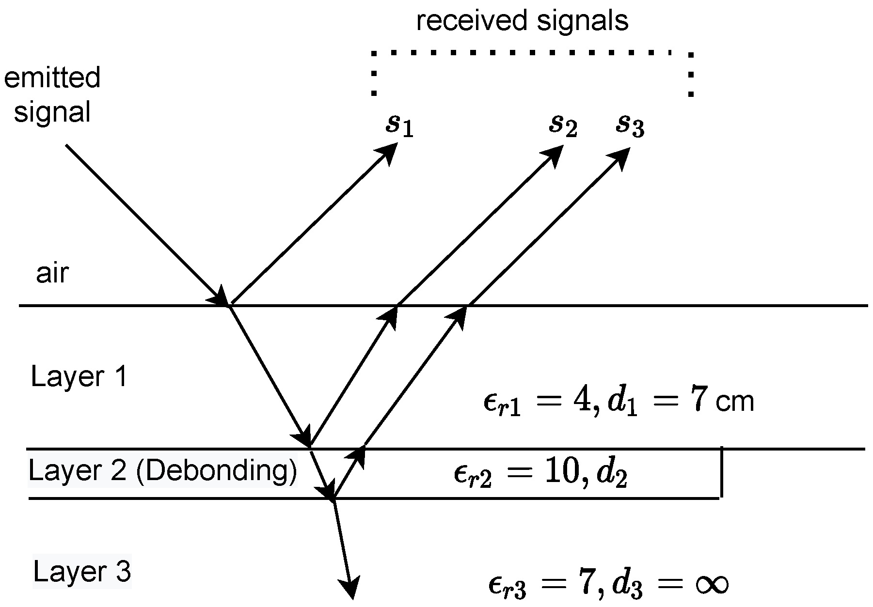
The rest of the paper is organized as follows. The GPR data model taking the shape of the transmitted radar pulse into account is presented in Section 2. Section 3 briefly reviews the principle of root-MUSIC for TDE and details the adaptation of PUMA to process the data model in Section 2 for TDE. In Section 4 and Section 5, the performance of both algorithms is compared in terms of the robustness to noise, time resolution, and average computational time. Conclusions and perspectives are given in Section 6.

Notation: Throughout this paper, vectors and matrices are denoted by lowercase and uppercase boldface letters, respectively. ${(·)}^{*}$, ${[·]}^T$, ${(·)}^H$, ${(·)}^{-1}$, and ${(·)}^{†}$ represent the complex conjugate, transpose, conjugate-transpose, matrix inverse, and pseudo inverse operations, respectively. $E[·]$ is the statistical mean. ⊗ is the Kronecker product. $vec(·)$ is the vectorization operator. $tr(·)$ is the trace operator. $\widehat{\mathbf{a}}$ represents the estimate of $\mathbf{a}$. $diag(·)$ denotes a diagonal matrix. ${\mathbf{I}}_m$ is the $(m,m)$ identity matrix, and ${\mathbf{J}}_m$ is the $(m,m)$ exchange matrix with ones on its antidiagonal and zeros elsewhere. ${\left[\mathbf{a}\right]}_m$ refers to the $m^{th}$ element of any vector $\mathbf{a}$.

2. Data Model

Let us consider a road pavement probed by a GPR at vertical incidence under the following assumptions:

• The road pavement is a stratified medium consisting of K smooth and homogeneous layers with low permittivity and negligible electrical conductivity;
• The impinging EM waves on the road pavement are assumed to be plane waves emitted from an antenna in the far field;
• Each layer contributes only one echo to the data model (single scattering assumption).

The backscattered signal recorded by the GPR under the above assumptions is the sum of the shifted and attenuated copies of the emitted radar pulse. The amplitude of each echo depends on the permittivity of the layers through Fresnel reflection coefficients. The received signal can be expressed as follows in the frequency domain [3,33]:

$$\tilde{y}\left(f_i\right)=\sum _{k=1}^K{s}_k\tilde{e}\left(f_i\right)e^{-j2\pi f_i{\tau }_k}+\tilde{n}\left(f_i\right)$$

(1)

where $s_k$ is the amplitude of the $k^{th}$ echo, which is considered to be independent of the frequency because the pavement layers have smooth interfaces, and $\tilde{e}\left(f_i\right)$ and $\tilde{n}\left(f_i\right)$ are the Fourier transforms of the emitted and noise signals, respectively. Equation (1) can be written in matrix form as:

$$\mathbf{y}=\mathbf{\Lambda }\mathbf{A}\mathbf{s}+\mathbf{n}$$

(2)

with:

• $\mathbf{y}={[\tilde{y}\left(f_1\right),\tilde{y}\left(f_2\right),...,\tilde{y}\left(f_N\right)]}^T$: $(N,1)$ frequency data vector;
• $\mathbf{\Lambda }=diag(\tilde{e}\left(f_1\right),\tilde{e}\left(f_2\right),...,\tilde{e}\left(f_N\right))$: $(N,N)$ diagonal matrix whose elements are the Fourier transforms of the emitted pulse;
• $\mathbf{A}=[\mathbf{a}\left({\tau }_1\right),\mathbf{a}\left({\tau }_2\right),...,\mathbf{a}\left({\tau }_K\right)]$: $(N,K)$ mode matrix;
• $\mathbf{a}\left({\tau }_k\right)={[e^{-j2\pi f_1{\tau }_k},e^{-j2\pi f_2{\tau }_k},...,e^{-j2\pi f_N{\tau }_k}]}^T$: steering vector of size $(N,1)$;
• $\mathbf{s}={[s_1,s_2,...,s_K]}^T$: $(K,1)$ source vector containing the amplitudes of the echoes;
• $\mathbf{n}={[\tilde{n}\left(f_1\right),\tilde{n}\left(f_2\right),...,\tilde{n}\left(f_N\right)]}^T$: $(N,1)$ noise vector with zero mean and covariance matrix ${\sigma }^2{\mathbf{I}}_N$;
• $f_i=f_1+(i-1)\Delta f$: the frequency samples where $f_1$ is the beginning of the bandwidth, $\Delta f$ is the frequency difference between two adjacent samples, and $i=1,2,\cdots ,N$.

The data covariance matrix $\mathbf{\Gamma }$ can be written as:

$$\mathbf{\Gamma }=E\left[\mathbf{y}{\mathbf{y}}^H\right]=\mathbf{\Lambda }\mathbf{A}{\mathbf{\Gamma }}_s{\mathbf{A}}^H{\mathbf{\Lambda }}^H+{\sigma }^2{\mathbf{I}}_N$$

(3)

where ${\mathbf{\Gamma }}_s=E\left[\mathbf{s}{\mathbf{s}}^H\right]$ and ${\sigma }^2{\mathbf{I}}_N=E\left[\mathbf{n}{\mathbf{n}}^H\right]$ are the covariance matrices of the source vector and the noise vector, with dimensions $(K,K)$ and $(N,N)$, respectively.

Compared to the conventional model in the literature, the magnitude variations of the radar pulse over the bandwidth are taken into account in the data model and the covariance matrix in (1) and (3), respectively. For the GPR configuration used in this application, the backscattered echoes consist of multipath from the same transmitter (Tx). The echoes in the source vector $\mathbf{s}$ are then expected to be highly correlated with each other, and the associated covariance matrix ${\mathbf{\Gamma }}_s$ may be rank deficient, i.e., $1\le rank\left({\mathbf{\Gamma }}_s\right)\le K$. Different correlation scenarios are thus considered in Section 4 for testing the TDE algorithms presented in the next section.

3. Time Delay Estimation Algorithms

This section presents two root-finding algorithms that are used in Section 4 to process GPR data for TDE. Firstly, the well-known root-MUSIC algorithm is recalled, and then, the proposed adaptation of PUMA to TDE is presented. Both algorithms take advantage of the eigendecomposition of the covariance matrix in different ways in order to estimate the time delays of the echoes.

3.1. Eigendecomposition

Assuming that ${\mathbf{\Gamma }}_s$ is of full rank, without loss of generality (in the case where the sources are totally coherent, the sub-band averaging techniques can be used for recovering the rank of ${\mathbf{\Gamma }}_s$), the covariance matrix of the received signal can be expressed as follows after eigendecomposition:

$$\mathbf{\Gamma }={\mathbf{E}}_s{\mathbf{D}}_s{\mathbf{E}}_s^H+{\mathbf{E}}_n{\mathbf{D}}_n{\mathbf{E}}_n^H$$

(4)

where the columns of ${\mathbf{E}}_s=[{\mathbf{u}}_1,\cdots ,{\mathbf{u}}_K]$, which are the eigenvectors associated with the first K largest eigenvalues in ${\mathbf{D}}_s=diag({\lambda }_1,\cdots ,{\lambda }_K)$, span the signal subspace and the columns of ${\mathbf{E}}_n=[{\mathbf{u}}_{K+1},\cdots ,{\mathbf{u}}_N]$, which are the eigenvectors associated with the $N-K$ smallest eigenvalues in ${\mathbf{D}}_n=diag({\lambda }_{K+1},\cdots ,{\lambda }_N)$, span the noise subspace. The eigenvalues are arranged in decreasing order: ${\lambda }_1>\cdots >{\lambda }_K>{\lambda }_{K+1}=\cdots ={\lambda }_N={\sigma }^2$.

Using (3) and (4),

$$\mathbf{\Gamma }-{\sigma }^2{\mathbf{I}}_N=\mathbf{\Lambda }\mathbf{A}{\mathbf{\Gamma }}_s{\mathbf{A}}^H{\mathbf{\Lambda }}^H={\mathbf{E}}_s({\mathbf{D}}_s-{\sigma }^2{\mathbf{I}}_K){\mathbf{E}}_s^H.$$

(5)

From (5),

$${\mathbf{E}}_s=\mathbf{\Lambda }\mathbf{A}\mathbf{T}\Rightarrow \mathbf{A}={\mathbf{\Lambda }}^{-1}{\mathbf{E}}_s{\mathbf{T}}^{-1}$$

(6)

where $\mathbf{T}$ is a nonsingular matrix of dimension $(K,K)$. Equation (6) means that $span\left(\mathbf{\Lambda }\mathbf{A}\right)=span\left({\mathbf{E}}_s\right)\Rightarrow span\left(\mathbf{A}\right)=span\left({\mathbf{\Lambda }}^{-1}{\mathbf{E}}_s\right)$.

3.2. Root-MUSIC

MUSIC is a well-known subspace method, which was adapted to TDE for processing GPR data in [3]. It is based on the orthogonality between the signal subspace, spanned by the columns of $\mathbf{\Lambda }\mathbf{A}$, and the noise subspace generated by the columns of ${\mathbf{E}}_n=[{\mathbf{u}}_{K+1},\cdots ,{\mathbf{u}}_N]$. For the data model in (3), MUSIC searches for the K time delays that minimize the following function:

$$F_M\left(\tau \right)=\mathbf{a}{\left(\tau \right)}^H{\mathbf{\Lambda }}^H{\mathbf{E}}_n{\mathbf{E}}_n^H\mathbf{\Lambda }\mathbf{a}\left(\tau \right).$$

(7)

The polynomial version of MUSIC, namely root-MUSIC, achieves better performance with a lower computational burden. Root-MUSIC searches for the complex roots z of the following $2N-2$-degree polynomial:

$$F_{RM}\left(z\right)={\mathbf{d}}^T(1/z){\mathbf{\Lambda }}^H{\mathbf{E}}_n{\mathbf{E}}_n^H\mathbf{\Lambda }\mathbf{d}\left(z\right)$$

(8)

where $\mathbf{d}\left(z\right)={\left[1,z,\dots ,z^{N-1}\right]}^T$ and $z=e^{-2j\pi \Delta f\tau }$.

The time delays are estimated from the phases of the K roots ${\widehat{z}}_k$ of $F_{RM}\left(z\right)$ closest to and inside the unit circle as follows:

$${\widehat{\tau }}_k=-\frac{\angle {\widehat{z}}_k}{2\pi \Delta f},1\le k\le K.$$

(9)

3.3. PUMA for TDE

In contrast to root-MUSIC, PUMA is an iterative subspace method [35,36]. According to the literature, PUMA may be directly applied to raw GPR data without preprocessing because it is more robust in the presence of correlated sources. In addition, it achieves a similar performance to that of conventional subspace methods in the presence of uncorrelated sources and has a lower average computational cost.

PUMA relies on linear prediction theory to estimate the time delays in the mode matrix $\mathbf{A}$. $\mathbf{A}$ has a Vandermonde structure; thus, the following orthogonal relation holds [35]

$$\mathbf{B}\mathbf{A}=\mathbf{0}$$

(10)

where:

$$\mathbf{B}=\left[\begin{array}{cccccc}{c}_K& c_{K-1}& \cdots & c_0& & 0\\ & \ddots & \ddots & & \ddots & & \\ 0& & c_K& c_{K-1}& \cdots & c_0\end{array}\right]$$

(11)

is an $(N-K,N)$ Toeplitz matrix. The coefficients of $\mathbf{B}$ define a polynomial with roots lying on the unit circle as follows [35]:

$$c_0{z}^K+c_1{z}^{K-1}+\cdots +c_K=c_0\prod _{k=1}^K(z-e^{-j2\pi \Delta f{\tau }_k})=0$$

(12)

where $c_0\ne 0$. Let $c_0=1$ and $\mathbf{c}={[c_1,c_2,\cdots ,c_K]}^T$; the time delays are estimated from the phases of the K roots of (12) with the use of (9).

Equation (10) also implies that each $m^{th}$ element ($m\ge K+1$) in the $k^{th}$ column of $\mathbf{A}$ can be written as a linear combination of the previous K elements in that column as:

$${\left[\mathbf{a}\left({\tau }_k\right)\right]}_m+\sum _{i=1}^K{c}_i{\left[\mathbf{a}\left({\tau }_k\right)\right]}_{m-i}=0,m\ge K+1;1\le k\le K.$$

(13)

In practice, we do not have access to $\mathbf{A}$. However, following (6), the columns of matrix ${\mathbf{\Lambda }}^{-1}{\mathbf{E}}_s$ span the same subspace generated by the columns of the mode matrix $\mathbf{A}$ in the absence of noise. Let:

$${\mathbf{\Lambda }}^{-1}{\mathbf{E}}_s=[{\mathbf{v}}_1,\cdots ,{\mathbf{v}}_K];$$

(14)

thus, (13) can be rewritten as:

$${\left[{\mathbf{v}}_k\right]}_m+\sum _{i=1}^K{c}_i{\left[{\mathbf{v}}_k\right]}_{m-i}=0,m\ge K+1;1\le k\le K.$$

(15)

Apart from the modification in (14), the rest of the algorithm is similar to that in [35]. For the completeness of presentation, the different steps of the algorithm are briefly recalled.

Equation (15) can be written in matrix form as:

$$\left[\begin{array}{cccc}{\left[{\mathbf{v}}_k\right]}_K& {\left[{\mathbf{v}}_k\right]}_{K-1}& \cdots & {\left[{\mathbf{v}}_k\right]}_1\\ [{\mathbf{v}}_k{]}_{K+1}& {\left[{\mathbf{v}}_k\right]}_K& \cdots & {\left[{\mathbf{v}}_k\right]}_2\\ ⋮& ⋮& & ⋮\\ {\left[{\mathbf{v}}_k\right]}_{N-1}& {\left[{\mathbf{v}}_k\right]}_{N-2}& \cdots & {\left[{\mathbf{v}}_k\right]}_{N-K}\end{array}\right]\left[\begin{array}{c}{c}_1\\ c_2\\ ⋮\\ c_K\end{array}\right]+\left[\begin{array}{c}{\left[{\mathbf{v}}_k\right]}_{K+1}\\ [{\mathbf{v}}_k{]}_{K+2}\\ ⋮\\ [{\mathbf{v}}_k{]}_N\end{array}\right]=\mathbf{0}$$

with:

$${\mathbf{F}}_k=\left[\begin{array}{cccc}{\left[{\mathbf{v}}_k\right]}_K& {\left[{\mathbf{v}}_k\right]}_{K-1}& \cdots & {\left[{\mathbf{v}}_k\right]}_1\\ [{\mathbf{v}}_k{]}_{K+1}& {\left[{\mathbf{v}}_k\right]}_K& \cdots & {\left[{\mathbf{v}}_k\right]}_2\\ ⋮& ⋮& & ⋮\\ {\left[{\mathbf{v}}_k\right]}_{N-1}& {\left[{\mathbf{v}}_k\right]}_{N-2}& \cdots & {\left[{\mathbf{v}}_k\right]}_{N-K}\end{array}\right]$$

(16)

$${\mathbf{g}}_k=-{[{\left[{\mathbf{v}}_k\right]}_{K+1},\dots ,{\left[{\mathbf{v}}_k\right]}_N]}^T$$

(17)

We can then write:

$${\mathbf{F}}_k\mathbf{c}-{\mathbf{g}}_k={\mathbf{0}}_{\left(\right(N-K),1)},1\le k\le K$$

(18)

and:

$$vec\left(\mathbf{B}{\mathbf{\Lambda }}^{-1}{\mathbf{E}}_s\right)=\mathbf{F}\mathbf{c}-\mathbf{g}={\mathbf{0}}_{\left(\right(N-K)K,1)}$$

(19)

where:

$$\mathbf{F}={\left[\begin{array}{c}{\mathbf{F}}_1\\ {\mathbf{F}}_2\\ ⋮\\ {\mathbf{F}}_K\end{array}\right]}_{\left(\right(N-K)K,K)},\mathbf{g}={\left[\begin{array}{c}{\mathbf{g}}_1\\ {\mathbf{g}}_2\\ ⋮\\ {\mathbf{g}}_K\end{array}\right]}_{\left(\right(N-K)K,1).}$$

Vector $\mathbf{c}$ can be found by solving:

$$\underset{\mathbf{c}}{min}{\parallel \mathbf{Fc}-\mathbf{g}\parallel }_2^2=\underset{\mathbf{c}}{min}{\parallel \mathbf{e}\parallel }_2^2=\underset{\mathbf{c}}{min}{\mathbf{e}}^H\mathbf{e}.$$

(20)

The least squares estimate of $\mathbf{c}$ can be obtained as:

$${\widehat{\mathbf{c}}}_{LS}={\left({\mathbf{F}}^H\mathbf{F}\right)}^{-1}{\mathbf{F}}^H\mathbf{g}={\mathbf{F}}^{†}\mathbf{g}.$$

(21)

However, in the presence of noise, (21) gives a biased estimate of $\mathbf{c}$, which eventually leads to inaccurate time delay estimates.

PUMA proposes to use weighted least squares to find $\mathbf{c}$. It solves [35,36]:

$$\underset{\mathbf{c}}{min}{\widehat{\mathbf{e}}}^H\widehat{\mathbf{W}}\widehat{\mathbf{e}}$$

(22)

where $\widehat{\mathbf{e}}=\widehat{\mathbf{F}}\mathbf{c}-\widehat{\mathbf{g}}$ and $\widehat{\mathbf{W}}$ is an estimate of the weighting matrix. $\widehat{\mathbf{W}}$ is of dimension $\left(\right(N-K)K,(N-K\left)K\right)$, and it is defined as:

$$\widehat{\mathbf{W}}={\left(E\left(\widehat{\mathbf{e}}{\widehat{\mathbf{e}}}^H\right)\right)}^{-1}\approx \widehat{\mathbf{T}}\otimes {\left(\mathbf{B}{\left(\mathbf{B}\right)}^H\right)}^{-1}$$

(23)

where $\widehat{\mathbf{T}}$ is a diagonal matrix defined as:

$$\widehat{\mathbf{T}}\approx diag\left(\frac{{({\widehat{\lambda }}_1-{\widehat{\sigma }}^2)}^2}{{\widehat{\lambda }}_1},\cdots ,\frac{{({\widehat{\lambda }}_K-{\widehat{\sigma }}^2)}^2}{{\widehat{\lambda }}_K}\right)$$

(24)

with ${\widehat{\sigma }}^2=\frac{1}{N-K}tr\left({\widehat{\mathbf{D}}}_n\right)$.

The WLS solution to (22) is given by [35,36,38]:

$${\widehat{\mathbf{c}}}_{WLS}={\left({\widehat{\mathbf{F}}}^H\widehat{\mathbf{W}}\widehat{\mathbf{F}}\right)}^{-1}{\widehat{\mathbf{F}}}^H\widehat{\mathbf{W}}\widehat{\mathbf{g}}.$$

(25)

It can be seen that (25) cannot be used directly because $\widehat{\mathbf{W}}$ depends on $\mathbf{c}$; thus, an initial value of $\mathbf{c}$ needs to be found. The following steps summarize PUMA for TDE:

• Initialize $\mathbf{c}$ with the least squares solution in (21): $\widehat{\mathbf{c}}={\widehat{\mathbf{c}}}_{LS}$;
• Calculate the weighting matrix $\widehat{\mathbf{W}}$ with $\widehat{\mathbf{c}}$ using (11) and (23);
• Calculate the WLS solution of $\widehat{\mathbf{c}}$, ${\widehat{\mathbf{c}}}_{WLS}$ with (25);
• Let $\widehat{\mathbf{c}}={\widehat{\mathbf{c}}}_{WLS}$, and repeat Steps 2 and 3 until ${\parallel \widehat{\mathbf{c}}-{\widehat{\mathbf{c}}}_{WLS}\parallel }_2$ becomes stable.

It was found that 3 iterations of Steps 2 and 3 were enough to satisfy the condition in Step 4 [36]. The time delays were estimated from (9) after finding the K roots of (12) with $\widehat{\mathbf{c}}$ obtained from the steps described above.

4. Simulated Data

In this section, the parameters used to simulate the GPR data over a simplified debonded pavement structure are presented. They serve to compute the data covariance matrices that are processed by the two selected TDE algorithms. In order to test the robustness of the selected algorithms within a multipath background, three different correlation scenarios were introduced, and two modified sub-band averaging techniques are proposed in Appendix A and Appendix B to mitigate the influence of coherent sources.

4.1. Parameters for the Pavement Survey

As shown in Figure 1, the defected pavement was modeled as a layered structure in which the debonding (Layer 2) was a thin layer with relative permittivity ${ϵ}_{r2}=10$ embedded between Layer 1 and Layer 3, with relative permittivities ${ϵ}_{r1}=4$ and ${ϵ}_{r3}=7$, respectively. The pavement structure was probed with an air-coupled step-frequency GPR, of which the pulse was modeled as a Ricker pulse with processed bandwidth $B=3 \mathrm{G}\mathrm{Hz}$ ($[0.7-3.7]$ GHz) and $f_c=2.2 \mathrm{G}\mathrm{Hz}$ as the central frequency. $N=150$ frequency samples were considered in the data vector. The noise was assumed to be white Gaussian. The thickness of Layer 1 was taken as $d_1=7 \mathrm{c}\mathrm{m}$, and that of Layer 3 was considered infinite. In the RMSE versus SNR simulations, the debonding region was set to $d_2=0.5 \mathrm{c}\mathrm{m}$; thus, the times of arrival associated with the backscattered echoes from the top surfaces of Layer 1, the debonding region, and Layer 3 were $[{\tau }_1,{\tau }_2,{\tau }_3]=[2.0,2.9,3.0]\mathrm{n}\mathrm{s}$, respectively. The amplitudes of the backscattered echoes from Layer 1, the debonding, and Layer 3 were found to be $s_1=-0.333$, $s_2=-0.200$, and $s_3=0.075$, respectively, from the Fresnel equations. Figure 2 displays the shape of the Ricker pulse and the noiseless simulated signals over the debonded ($d_2=0.5 \mathrm{c}\mathrm{m}$) and the healthy areas.

To test the time resolution capability of the selected TDE algorithms in Section 5, the debonding thickness $d_2$ was varied from $0.05$ $\mathrm{c}$$\mathrm{m}$ to $3.97$ $\mathrm{c}$$\mathrm{m}$, corresponding to a variation of $B\Delta T_2$ from 0.03 to 2.51, with $\Delta T_2={\tau }_3-{\tau }_2$. Conventional FFT-based methods can easily resolve echoes when $B\Delta T\ge 1$, but they fail to detect overlapping echoes, i.e., $B\Delta T<1$.

4.2. Correlation Scenarios

The two selected algorithms were performed on the simulated data covariance matrix in (3). To test the robustness of the algorithms, the following three simulation scenarios were considered by varying the correlation coefficients in the source covariance matrix ${\mathbf{\Gamma }}_s$ in (3), which is defined for three echoes as follows:

$${\mathbf{\Gamma }}_s=\left[\begin{array}{ccc}|s_1{|}^2& {\rho }_{12}|s_1\left|\right|s_2|& {\rho }_{13}|s_1\left|\right|s_3|\\ {\rho }_{12}^{*}|s_1\left|\right|s_2|& |s_2{|}^2& {\rho }_{23}|s_2\left|\right|s_3|\\ {\rho }_{13}^{*}|s_1\left|\right|s_3|& {\rho }_{23}^{*}|s_2\left|\right|s_3|& |s_3{|}^2\end{array}\right]$$

(26)

where $s_k$ with $k=\{1,2,3\}$ are the amplitudes of the echoes and ${\rho }_{ij}$ are the correlation coefficients between the $i^{th}$ and $j^{th}$ echoes (with $i=\{1,2,3\}$, $j=\{1,2,3\}$, $i\ne j$).

4.2.1. Scenario 1: Uncorrelated Echoes

This scenario investigated the best performance of the selected algorithms by assuming that the 3 backscattered echoes were fully uncorrelated. This correlation scenario was believed to match to the performance achieved by the Cramer–Rao bound. The full rank data covariance matrix corresponding to this case was simulated by setting ${\rho }_{12}={\rho }_{13}={\rho }_{23}=0$ in (26).

4.2.2. Scenario 2: Full Correlation between Overlapping Echoes

In this scenario, the last two echoes were correlated with each other while uncorrelated with the first one; thus, ${\rho }_{12}={\rho }_{13}=0$ and ${\rho }_{23}=1$ in (26). This scenario is similar to the first simulation carried out by Qian et al. in [35] within the scope of DOA application. It was expected to be closer to what can be observed in practice for the GPR application under scope, because the second and third echoes strongly overlapped.

4.2.3. Scenario 3: Full Correlation between Echoes

In this case, the three backscattered echoes were considered to be fully correlated; thus, ${\rho }_{12}={\rho }_{13}={\rho }_{23}=1$, reducing the rank of the covariance matrix of sources ${\mathbf{\Gamma }}_s$ to 1. Compared to Scenarios 1 and 2, this scenario was expected to be the closest to the GPR experiment, where the backscattered echoes originated from the same transmitter.

4.3. Computed Data Covariance Matrix

The signal parameters in Section 4.1 were used to compute the data covariance matrix $\mathbf{\Gamma }$ in (3) that were processed by the two selected TDE algorithms. The noise covariance matrix is estimated from I independent snapshots as follows:

$${\widehat{\mathbf{\Gamma }}}_{noise}=\frac{1}{I}\mathbf{N}{\mathbf{N}}^H$$

(27)

where $\mathbf{N}=[{\mathbf{n}}_1,\cdots ,{\mathbf{n}}_I]$ is the noise data matrix.

To mitigate the influence of coherent sources in Scenarios 2 and 3, TDE was also performed on the modified FB (forward–backward) data covariance matrix (${\mathbf{\Gamma }}_{\Lambda }^{FB}$) and the modified MSSP (modified spatial smoothing processing) data covariance matrix (${\mathbf{\Gamma }}_{\Lambda }^{MSSP}$), which are detailed in Appendix A and Appendix B, respectively. Both matrices rely on the well-known FB and MSSP sub-band averaging techniques [41,42]. The two proposed techniques avoid some limitations of the conventional FB and MSSP techniques when they are applied to the GPR data model in (2).

FB applies the averaging technique only once over the whole GPR bandwidth in both the forward and backward directions. For MSSP, the averaging technique was performed over overlapping frequency sub-bands of size L. According to [3], MSSP performs best when the effective bandwidth ratio $L/N$ is between 80% and 90%. In this paper, $L/N$ = 80% was chosen.

5. Results

In this section, the performance of the proposed PUMA algorithm is compared to root-MUSIC for the three correlation scenarios introduced in the previous section.

5.1. Evaluation Criteria

The selected algorithms were compared in terms of the root-mean-squared error (RMSE) versus the signal-to-noise ratio (SNR), the RMSE versus $B\Delta T_2$, and average computational time. The RMSE was focused on the two overlapping echoes to expect more sensitive results, and it is computed as follows:

$$RMSE={\left(\frac{1}{2I}\sum _{k=2}^3\sum _{i=1}^I{({\widehat{\tau }}_{k,i}-{\tau }_k)}^2\right)}^{1/2}$$

(28)

where ${\widehat{\tau }}_{k,i}$ is the $k^{th}$ time delay estimate obtained from the $i^{th}$ test and ${\tau }_k$ is the true $k^{th}$ time delay. $I=100$ is the number of Monte Carlo tests. For this application, the SNR is defined as the ratio between the sum of the squared magnitude of the two overlapping echoes to that of the noise power:

$$SNR=\frac{{\left|s_2\right|}^2+{\left|s_3\right|}^2}{{\sigma }^2}.$$

(29)

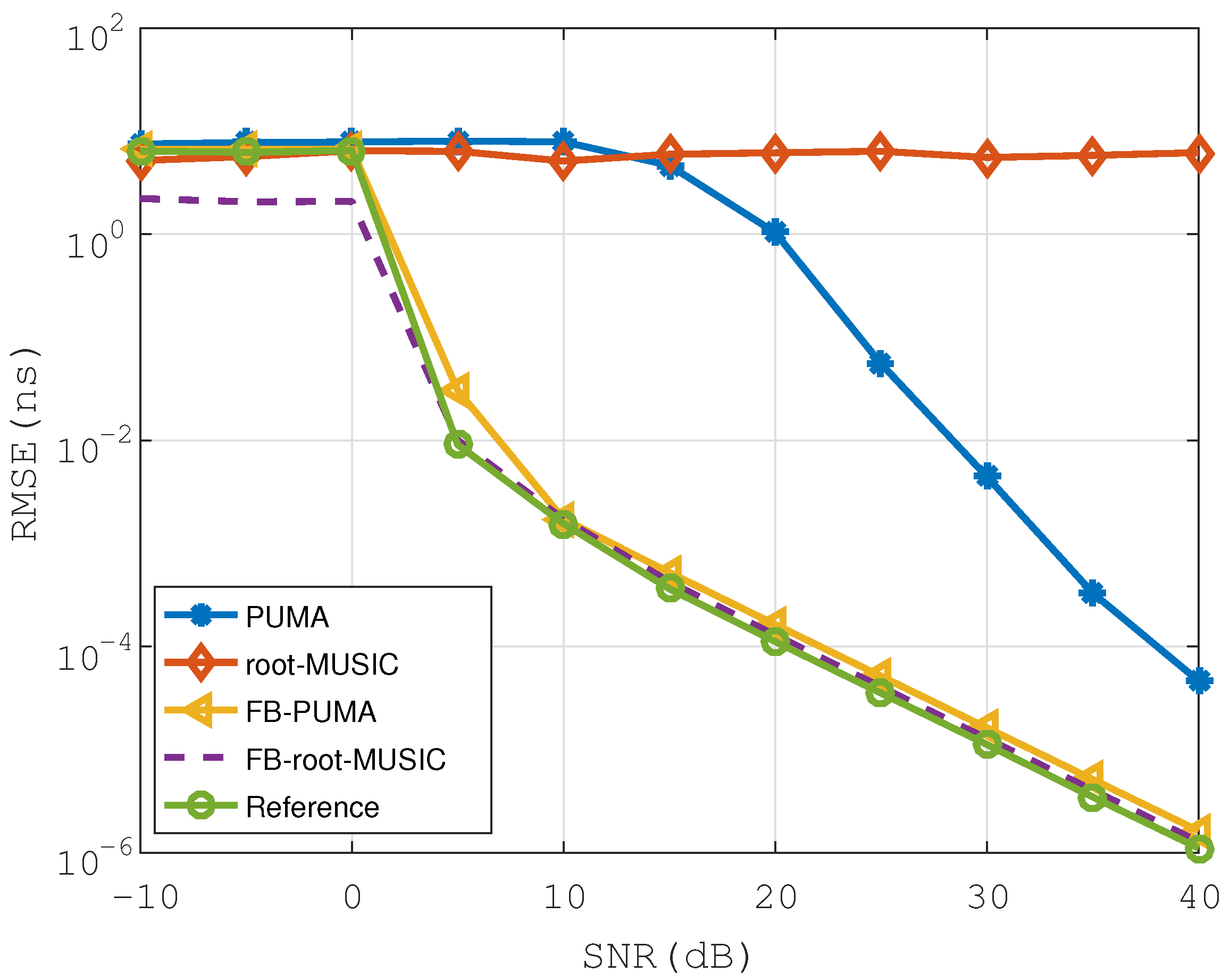
5.2. Scenario 1: Uncorrelated Echoes

Figure 3 and Figure 4 show the RMSE versus the SNR and the RMSE versus $B\Delta T_2$ plots, respectively. It can be seen from Figure 3 that root-MUSIC is more robust to noise than PUMA. At SNRs $\ge 10$ dB, the performance of PUMA approaches that of root-MUSIC. From Figure 4, it can be concluded that the selected algorithms can successfully resolve the two overlapping echoes from the debonding with root-MUSIC having better resolution capabilities than PUMA for SNR $=25$ dB. The RMSE plots of root-MUSIC are used as the benchmark in the next scenarios.

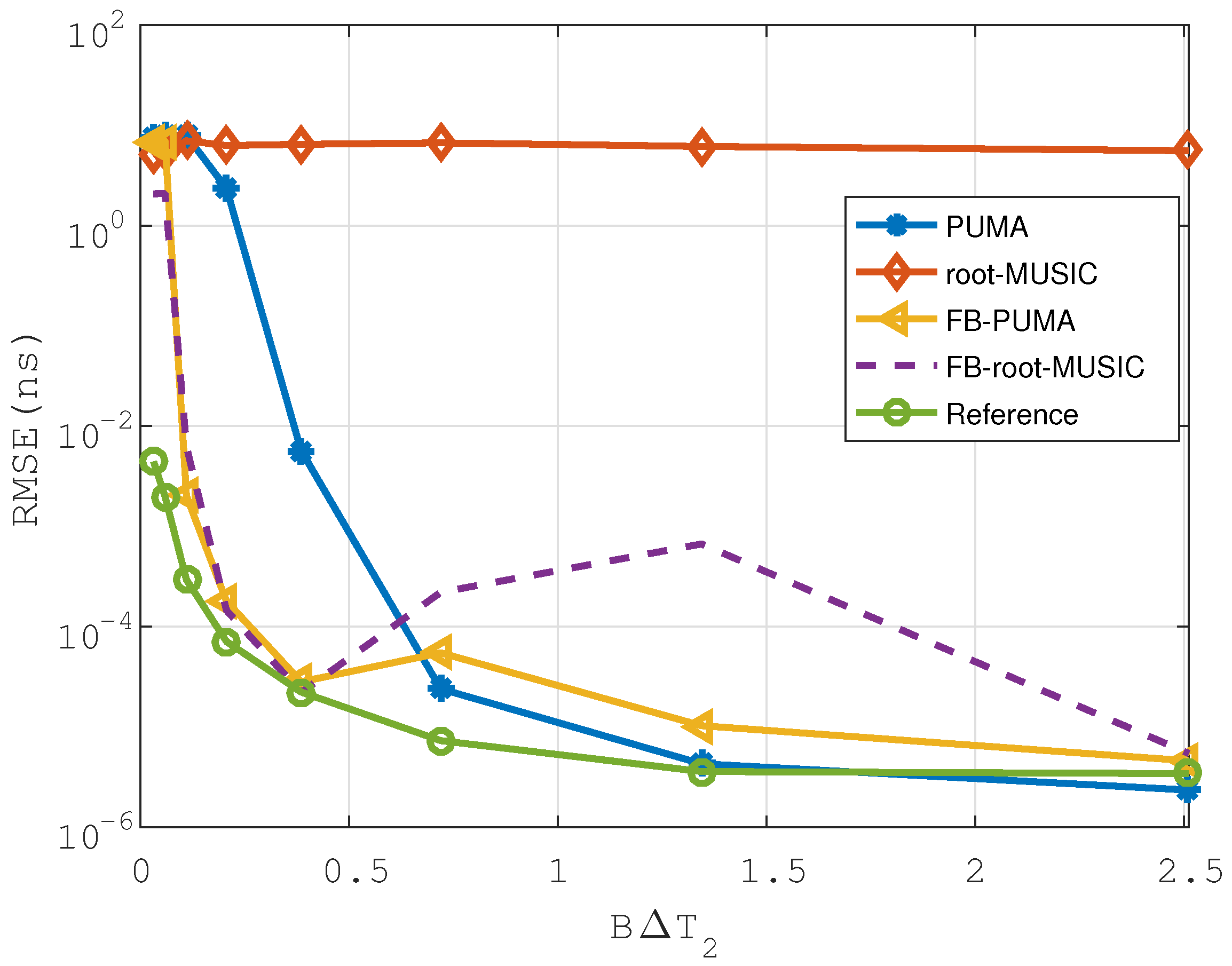
5.3. Scenario 2: Full Correlation between the Overlapping Echoes

The two selected algorithms were successively applied on the data covariance matrix in (3) and on the FB data covariance matrix ${\mathbf{\Gamma }}_{\Lambda }^{FB}$ defined in (A6). During the processing of the former and the latter, (8) and (14) were computed using the pulse matrix $\mathbf{\Lambda }$ in (2) and ${\mathbf{\Lambda }}_{FB}$ derived from (A4), respectively. The RMSE versus the SNR and the RMSE versus $B\Delta T_2$ plots are shown in Figure 5 and Figure 6, respectively.

As expected, root-MUSIC failed to work on the covariance data matrix in (3), because it had a reduced rank equal to two. By contrast, PUMA succeeded in TDE for SNRs $\ge 20$ dB, as shown in Figure 5, and likely achieved the best performance at a very high SNR.

The FB-root-MUSIC and FB-PUMA approach had the best performance, with FB-root-MUSIC performing better than FB-PUMA. The former and the latter outperformed root-MUSIC and PUMA because forward–backward averaging restored the rank of ${\mathbf{\Gamma }}_s$. It is worth noticing that under this scenario, the performance of PUMA in [35] corresponds to that of FB-PUMA in our paper.

The time resolution of both algorithms is displayed in Figure 6. Figure 6 shows that only PUMA can separate the overlapping echoes, i.e., for $B\Delta T_2<1$, when the algorithms are performed on the data covariance matrix. The time resolution of PUMA and root-MUSIC improved once they were applied to ${\mathbf{\Gamma }}_{\Lambda }^{FB}$. At $B\Delta T_2=0.3$ (i.e., $0.5$ $\mathrm{c}$$\mathrm{m}$), FB-PUMA and FB-root-MUSIC showed similar performance, and they both outperformed PUMA and root-MUSIC. However, the ultimate time resolution stayed lower than the one achieved with fully uncorrelated sources.

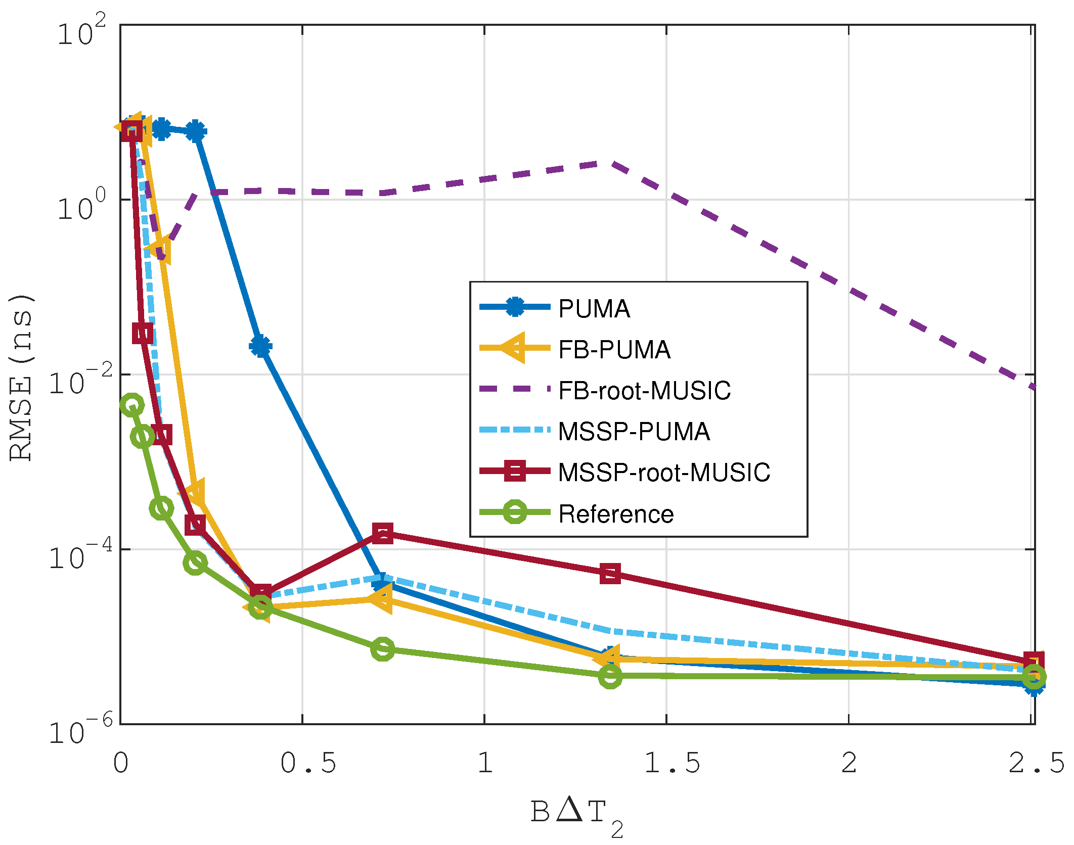
5.4. Scenario 3: Full Correlation between Echoes

As for Scenario 2, PUMA and root-MUSIC were successively applied on the data covariance matrix in (3), the FB data covariance matrix ${\mathbf{\Gamma }}_{\Lambda }^{FB}$ in (A6), and finally, the MSSP data covariance matrix ${\mathbf{\Gamma }}_{\Lambda }^{MSSP}$ in (A19). For MSSP, (8) and (14) were computed using ${\mathbf{\Lambda }}_{MSSP}$ derived from (A17).

Figure 7 and Figure 8 plot the RMSE of the selected algorithms versus the SNR and $B\Delta T_2$, respectively. The performance of root-MUSIC is not plotted because it does not work in the presence of correlated sources. As shown in Figure 7, FB-root-MUSIC failed to work because the FB averaging technique can handle at most two correlated sources. FB-PUMA worked for SNRs $>6$ dB, thus improving the performance of PUMA, which is limited to SNRs $>22$ dB. MSSP-PUMA and MSSP-root-MUSIC had a similar performance, and they both outperformed FB-PUMA, FB-root-MUSIC, and PUMA because ${\mathbf{\Gamma }}_{\Lambda }^{MSSP}$ was of full rank. Surprisingly, MSSP-PUMA and MSSP-root-MUSIC performed better than the reference algorithm at SNRs $<10$ dB, and MSSP was believed to improve the robustness to noise with its sub-band average.

Figure 8 shows that MSSP-PUMA and MSSP-root-MUSC outperformed FB-PUMA, PUMA, and FB-root-MUSIC when $B\Delta T_2\le 0.3$ at an SNR of $25$ dB. The “bumps” observed were due to the oscillations of the effective correlation coefficients obtained after the MSSP sub-band averaging technique. The magnitude of the “bumps” was smaller for PUMA owing to a better robustness against correlation.

Finally, in Figure 9, the average computational time of PUMA and root-MUSIC for SNR $=25$ dB is plotted against the size of the data vector N. N was varied from 50 to 300 samples, and the computational time at each number of samples was averaged over 100 runs. The computational time increased with respect to N for both algorithms, with PUMA being about 10-times faster than root-MUSIC. All the simulations were carried out on a PC with Intel Core i5, 4 GB RAM, and $2.5$ $\mathrm{GHz}$.

6. Conclusions

In this paper, PUMA was successfully adapted to the processing of GPR data for time delay estimation by directly taking into account the radar pulse form. Two important modified sub-band averaging techniques were introduced. The simulation results illustrated the use of PUMA for the detection of thin debondings within pavement structures from air-coupled GPR data. The performance of the proposed method was compared with the classical root-MUSIC method. In terms of robustness against noise and time resolution capability, PUMA achieved a similar performance to that of the reference in the ideal scenario, i.e., fully uncorrelated echoes, and lower performance compared to the reference in more realistic scenarios with correlated echoes. Besides, PUMA was found to be about 10-times faster than root-MUSIC. In any case, the achieved time resolution clearly proves that PUMA can meet the needs of the application under scope by detecting subcentimeter-thick debondings within a pavement structure. However, the simulation results suggested that the PUMA algorithm can be further enhanced in the case of fully correlated echoes, and this can be done by extending the PUMA algorithm to directly exploit the properties of the rank-deficient source covariance matrix. In the near future, it is planned to test PUMA on the existing field database in [43].

References

- Solla, M.; Pérez-Gracia, V.; Fontul, S. A Review of GPR Application on Transport Infrastructures: Troubleshooting and Best Practices. Remote Sens. 2021, 13, 672. [Google Scholar] [CrossRef]
- Saarenketo, T.; Scullion, T. Road evaluation with ground penetrating radar. J. Appl. Geophys. 2000, 43, 119–138. [Google Scholar] [CrossRef]
- Le Bastard, C.; Baltazart, V.; Wang, Y.; Saillard, J. Thin-pavement thickness estimation using GPR with high-resolution and superresolution methods. IEEE Trans. Geosci. Remote Sens. 2007, 45, 2511–2519. [Google Scholar] [CrossRef]
- Batrakov, D.O.; Antyufeyeva, M.S.; Antyufeyev, O.V.; Batrakova, A.G. GPR application for the road pavements surveys. In Proceedings of the 2017 IEEE Microwaves, Radar and Remote Sensing Symposium (MRRS), Kiev, Ukraine, 29–31 August 2017; pp. 81–84. [Google Scholar] [CrossRef]
- Marecos, V.; Fontul, S.; Solla, M.; de Lurdes Antunes, M. Evaluation of the feasibility of Common Mid-Point approach for air-coupled GPR applied to road pavement assessment. Measurement 2018, 128, 295–305. [Google Scholar] [CrossRef]
- Bianchini Ciampoli, L.; Tosti, F.; Economou, N.; Benedetto, F. Signal processing of GPR data for road surveys. Geosciences 2019, 9, 96. [Google Scholar] [CrossRef] [Green Version]
- Zhang, F.; Xie, X.; Huang, H. Application of ground penetrating radar in grouting evaluation for shield tunnel construction. Tunn. Undergr. Space Technol. 2010, 25, 99–107. [Google Scholar] [CrossRef]
- Alani, A.M.; Tosti, F. GPR applications in structural detailing of a major tunnel using different frequency antenna systems. Constr. Build. Mater. 2018, 158, 1111–1122. [Google Scholar] [CrossRef]
- Kilic, G.; Eren, L. Neural network based inspection of voids and karst conduits in hydro–electric power station tunnels using GPR. J. Appl. Geophys. 2018, 151, 194–204. [Google Scholar] [CrossRef]
- Lyu, Y.Z.; Wang, H.H.; Gong, J.B. GPR detection of tunnel lining cavities and reverse-time migration imaging. Appl. Geophys. 2020, 2020, 1–7. [Google Scholar] [CrossRef]
- Qin, H.; Zhang, D.; Tang, Y.; Wang, Y. Automatic recognition of tunnel lining elements from GPR images using deep convolutional networks with data augmentation. Autom. Constr. 2021, 130, 103830. [Google Scholar] [CrossRef]
- Solla, M.; Lorenzo, H.; Riveiro, B.; Rial, F. Non-destructive methodologies in the assessment of the masonry arch bridge of Traba, Spain. Eng. Fail. Anal. 2011, 18, 828–835. [Google Scholar] [CrossRef]
- Fauchard, C.; Antoine, R.; Bretar, F.; Lacogne, J.; Fargier, Y.; Maisonnave, C.; Guilbert, V.; Marjerie, P.; Thérain, P.F.; Dupont, J.P.; et al. Assessment of an ancient bridge combining geophysical and advanced photogrammetric methods: Application to the Pont De Coq, France. J. Appl. Geophys. 2013, 98, 100–112. [Google Scholar] [CrossRef]
- Morris, I.; Abdel-Jaber, H.; Glisic, B. Quantitative attribute analyses with ground penetrating radar for infrastructure assessments and structural health monitoring. Sensors 2019, 19, 1637. [Google Scholar] [CrossRef] [Green Version]
- Alsharqawi, M.; Zayed, T.; Shami, A. Ground Penetrating Radar-Based Deterioration Assessment of RC Bridge Decks; Construction Innovation: Bingley, UK, 2020. [Google Scholar] [CrossRef]
- Gagarin, N.; Goulias, D.; Mekemson, J.; Cutts, R.; Andrews, J. Development of Novel Methodology for Assessing Bridge Deck Conditions Using Step Frequency Antenna Array Ground Penetrating Radar. J. Perform. Constr. Facil. 2020, 34, 04019113. [Google Scholar] [CrossRef]
- Manacorda, G.; Morandi, D.; Sarri, A.; Staccone, G. Customized GPR system for railroad track verification. In Proceedings of the Ninth International Conference on Ground Penetrating Radar, Santa Barbara, CA, USA, 29 April–2 May 2002; Volume 4758, pp. 719–723. [Google Scholar] [CrossRef]
- Xiao, J.; Liu, L. Permafrost subgrade condition assessment using extrapolation by deterministic deconvolution on multifrequency GPR data acquired along the Qinghai-Tibet railway. IEEE J. Sel. Top. Appl. Earth Obs. Remote Sens. 2015, 9, 83–90. [Google Scholar] [CrossRef]
- De Bold, R.; O’connor, G.; Morrissey, J.; Forde, M. Benchmarking large scale GPR experiments on railway ballast. Constr. Build. Mater. 2015, 92, 31–42. [Google Scholar] [CrossRef] [Green Version]
- Bianchini Ciampoli, L.; Calvi, A.; D’Amico, F. Railway ballast monitoring by GPR: A test-site investigation. Remote Sens. 2019, 11, 2381. [Google Scholar] [CrossRef] [Green Version]
- Ranalli, D.; Scozzafava, M.; Tallini, M. Ground penetrating radar investigations for the restoration of historic buildings: The case study of the Collemaggio Basilica (L’Aquila, Italy). J. Cult. Herit. 2004, 5, 91–99. [Google Scholar] [CrossRef]
- Masini, N.; Persico, R.; Rizzo, E. Some examples of GPR prospecting for monitoring of the monumental heritage. J. Geophys. Eng. 2010, 7, 190–199. [Google Scholar] [CrossRef]
- Leucci, G.; Masini, N.; Persico, R. Time–frequency analysis of GPR data to investigate the damage of monumental buildings. J. Geophys. Eng. 2012, 9, S81–S91. [Google Scholar] [CrossRef]
- Pérez-Gracia, V.; Solla, M. Inspection procedures for effective GPR surveying of buildings. In Civil Engineering Applications of Ground Penetrating Radar; Springer: Berlin/Heidelberg, Germany, 2015; pp. 97–123. [Google Scholar]
- Hugenschmidt, J.; Kalogeropoulos, A. The inspection of retaining walls using GPR. J. Appl. Geophys. 2009, 67, 335–344. [Google Scholar] [CrossRef]
- Ukleja, J.; Bęben, D.; Anigacz, W. Determination of the railway retaining wall dimensions and its foundation in difficult terrain and utility. AGH J. Min. Geoengin. 2012, 36, 299–308. [Google Scholar]
- Solla, M.; González-Jorge, H.; Álvarez, M.X.; Arias, P. Application of non-destructive geomatic techniques and FDTD modeling to metrical analysis of stone blocks in a masonry wall. Constr. Build. Mater. 2012, 36, 14–19. [Google Scholar] [CrossRef]
- Beben, D.; Anigacz, W.; Ukleja, J. Diagnosis of bedrock course and retaining wall using GPR. NDT E Int. 2013, 59, 77–85. [Google Scholar] [CrossRef]
- Spagnolini, U. Permittivity measurements of multilayered media with monostatic pulse radar. IEEE Trans. Geosci. Remote Sens. 1997, 35, 454–463. [Google Scholar] [CrossRef] [Green Version]
- Simonin, J.M.; Baltazart, V.; Le Bastard, C.; Derobert, X. Progress in monitoring the debonding within pavement structures during accelerated pavement testing on the fatigue carousel. In Proceedings of the 8th RILEM International Conference on Mechanisms of Cracking and Debonding in Pavements, Nantes, France, 7–9 June 2016; pp. 749–755. [Google Scholar]
- Lai, W.W.L.; Derobert, X.; Annan, P. A review of Ground Penetrating Radar application in civil engineering: A 30-year journey from Locating and Testing to Imaging and Diagnosis. NDT E Int. 2018, 96, 58–78. [Google Scholar]
- Al-Qadi, I.L.; Lahouar, S. Measuring layer thicknesses with GPR–Theory to practice. Constr. Build. Mater. 2005, 19, 763–772. [Google Scholar] [CrossRef]
- Sun, M.; Pan, J.; Le Bastard, C.; Wang, Y.; Li, J. Advanced signal processing methods for ground-penetrating radar: Applications to civil engineering. IEEE Signal Process. Mag. 2019, 36, 74–84. [Google Scholar] [CrossRef] [Green Version]
- Barabell, A. Improving the resolution performance of eigenstructure-based direction-finding algorithms. In Proceedings of the ICASSP’83, IEEE International Conference on Acoustics, Speech, and Signal Processing, Boston, MA, USA, 14–16 April 1983; Volume 8, pp. 336–339. [Google Scholar] [CrossRef]
- Qian, C.; Huang, L.; Cao, M.; Xie, J.; So, H.C. PUMA: An improved realization of MODE for DOA estimation. IEEE Trans. Aerosp. Electron. Syst. 2017, 53, 2128–2139. [Google Scholar] [CrossRef]
- Chan, F.K.; So, H.C.; Sun, W. Subspace approach for two-dimensional parameter estimation of multiple damped sinusoids. Signal Process. 2012, 92, 2172–2179. [Google Scholar] [CrossRef] [Green Version]
- So, H.C.; Chan, F.K.; Lau, W.H.; Chan, C.F. An efficient approach for two-dimensional parameter estimation of a single-tone. IEEE Trans. Signal Process. 2009, 58, 1999–2009. [Google Scholar] [CrossRef] [Green Version]
- Qian, C.; Huang, L.; Sidiropoulos, N.D.; So, H.C. Enhanced PUMA for direction-of-arrival estimation and its performance analysis. IEEE Trans. Signal Process. 2016, 64, 4127–4137. [Google Scholar] [CrossRef]
- Shahimaeen, A.; Dehghani, M.J.; Dodangeh, M. Two-dimensional DOA estimation for noncoherent and coherent signals using subspace approach. Trans. Emerg. Telecommun. Technol. 2019, 30, 3752. [Google Scholar] [CrossRef]
- Haardt, M.; Nossek, J.A. Unitary ESPRIT: How to obtain increased estimation accuracy with a reduced computational burden. IEEE Trans. Signal Process. 1995, 43, 1232–1242. [Google Scholar] [CrossRef]
- Pesavento, M.; Gershman, A.B.; Haardt, M. Unitary root-MUSIC with a real-valued eigendecomposition: A theoretical and experimental performance study. IEEE Trans. Signal Process. 2000, 48, 1306–1314. [Google Scholar] [CrossRef]
- Yamada, H.; Ohmiya, M.; Ogawa, Y.; Itoh, K. Superresolution techniques for time-domain measurements with a network analyzer. IEEE Trans. Antennas Propag. 1991, 39, 177–183. [Google Scholar] [CrossRef]
- Dérobert, X.; Baltazart, V.; Simonin, J.M.; Todkar, S.S.; Norgeot, C.; Hui, H.Y. GPR Monitoring of Artificial Debonded Pavement Structures throughout Its Life Cycle during Accelerated Pavement Testing. Remote Sens. 2021, 13, 1474. [Google Scholar] [CrossRef]
Publisher’s Note: MDPI stays neutral with regard to jurisdictional claims in published maps and institutional affiliations. |
© 2021 by the authors. Licensee MDPI, Basel, Switzerland. This article is an open access article distributed under the terms and conditions of the Creative Commons Attribution (CC BY) license (https://creativecommons.org/licenses/by/4.0/).
Share and Cite
Tchana Tankeu, B.; Baltazart, V.; Wang, Y.; Guilbert, D. PUMA Applied to Time Delay Estimation for Processing GPR Data over Debonded Pavement Structures. Remote Sens. 2021, 13, 3456. https://doi.org/10.3390/rs13173456
Tchana Tankeu B, Baltazart V, Wang Y, Guilbert D. PUMA Applied to Time Delay Estimation for Processing GPR Data over Debonded Pavement Structures. Remote Sensing. 2021; 13(17):3456. https://doi.org/10.3390/rs13173456
Chicago/Turabian StyleTchana Tankeu, Bachir, Vincent Baltazart, Yide Wang, and David Guilbert. 2021. "PUMA Applied to Time Delay Estimation for Processing GPR Data over Debonded Pavement Structures" Remote Sensing 13, no. 17: 3456. https://doi.org/10.3390/rs13173456