Article

Comparative Analysis of PM2.5 and O3 Source in Beijing Using a Chemical Transport Model

1
School of Energy and Environmental Engineering, University of Science and Technology Beijing, Beijing 100083, China
2
State Key Laboratory of Severe Weather & Key Laboratory of Atmospheric Chemistry of CMA, Chinese Academy of Meteorological Sciences, Beijing 100081, China
3
National Meteorological Center, Beijing 100081, China
4
Institute of Urban Meteorology, China Meteorological Administration, Beijing 100081, China
*
Author to whom correspondence should be addressed.
Remote Sens. 2021, 13(17), 3457; https://doi.org/10.3390/rs13173457
Submission received: 12 May 2021 / Revised: 26 August 2021 / Accepted: 27 August 2021 / Published: 31 August 2021

Abstract

:
For many years, Beijing has suffered from severe air pollution. At present, fine particulate matter (PM2.5) pollution in the winter and ozone (O3) pollution in the summer constitute serious environmental problems. In this study, the combination of a comprehensive air quality model with particulate matter source apportionment technology (CAMx-PAST) and monitoring data was used for the high-spatial resolution source apportionment of secondary inorganic components (SNA: SO42, NO3, and NH4+) in PM2.5; their corresponding precursor gases (SO2, NO2, and NH3); and O3 in the winter and summer over Beijing. Emissions from residents, industry, traffic, agriculture, and power accounted for 54%, 25%, 14%, 5%, and 2% of PM2.5 in the winter, respectively. In the summer, the emissions from industry, traffic, residents, agriculture, and power accounted for 42%, 24%, 20%, 10%, and 4% of PM2.5, respectively. The monthly transport ratio of PM2.5 was 27% and 46% in the winter and summer, respectively. The regional transport of residential and industrial emissions accounted for the highest proportion of PM2.5. The regional transport of emissions had a significant effect on the SO42 and NO3 concentrations, whereas SO2 and NO2 pollution were mainly affected by local emissions, and NH4+ and NH3 were mainly attributed to agricultural emissions. Industrial and traffic sources were two major emission sectors that contributed to O3 pollution in Beijing. The monthly transport ratios of O3 were 31% and 65% in the winter and summer, respectively. The high-spatial resolution regional source apportionment results showed that emissions from Langfang, Baoding, and Tangshan had the greatest impact on Beijing’s air pollution. This work’s methods and results will provide scientific guidance to support the government in its decision-making processes to manage the PM2.5 and O3 pollution issues.

1. Introduction

Beijing, the capital of China, has undergone rapid socioeconomic change, which has placed tremendous pressure on the ecological environment and led to its deterioration. In recent decades, Beijing has suffered severe air pollution. At present, fine particulate matter (PM2.5) pollution in the winter and ozone (O3) pollution in the summer constitute severe environmental problems [1,2,3]. The unique terrain of Beijing, which is surrounded by the Yan Mountains to the northwest and the Taihang Mountains to the southwest, is conducive to trapping air pollution over the city [4]. To effectively control regional pollution and improve the air quality, central and local governments have implemented a series of air pollution control action plans since 1998. At that time, the annual ambient concentrations of SO2 and NO2 in Beijing were 120 μg m3 and 74 μg m3, respectively. In 1998, policies were launched to reduce the emissions from coal-fired power plants, residential heating, boilers, and traffic, and these measures showed positive trends toward improving the air quality. In 2013, the annual concentrations of SO2 and NO2 decreased to 26.5 μg m3 and 56.0 μg m3, respectively. PM10 and PM2.5 were also included in the ambient air quality monitoring scheme; and at that time, the annual PM10 and PM2.5 concentrations were 108 μg m3 and 89.5 μg m3, respectively [5]. In September 2013, the central government of China released the ‘National Action Plan for Air Pollution Prevention and Control’, which required the local Beijing government to reduce the annual PM2.5 concentration by 25% by 2017 [6]. In 2017, the Ministry of Ecology and Environment of the People’s Republic of China released the ‘Air Pollution Prevention and Control Action Plan for the Beijing-Tianjin-Hebei (BTH) and Surrounding Region’ [7]. This plan suggested that these provinces simultaneously carry out emission control measures during heavy pollution episodes and establish a regional control network to prevent air pollution. The central and local governments have thus taken great pains to improve the air quality. The annual PM2.5 concentration decreased from 89.5 μg m3 in 2013 to 58.0 μg m3 in 2017, demonstrating that the air quality in Beijing has continuously improved [8]. However, the complicated nonlinear chemistry involved in the formation of photochemical pollution and the reduction of NOx increases O3. Many studies have shown that O3 pollution is becoming increasingly prominent in the region [9,10]. It was reported that the O3 concentration on the North China Plain (NCP, including Beijing, Tian, and Hebei) increased from 2015 to 2018 with a growth rate of 22.84% [11], which reflects a serious situation of O3 pollution. It is important for Beijing to take proactive actions to coordinate the control of O3 and other pollutants and to improve the air quality. These practices also provide opportunities to conduct experiments to study the atmospheric chemical mechanisms over China.
A source apportionment method identifies potential emission sources of air pollution and examines the contribution of each source and region to the pollution concentration by using various approaches. Source apportionment is an indispensable prerequisite for the effective implementation of emission control strategies. This technique has been used by governments and scientific researchers to help understand air pollutants and develop emission control strategies. A number of air pollution source apportionment methods have been developed and applied in recent decades, and several types of source apportionment methods have been widely used. (1) Receptor-based approaches have been extensively applied, including principal component analysis models [12], positive matrix factorization (PMF) models [13,14], and chemical mass balance (CMB) models [15,16], which are based on the principle of mass conservation. Solving the mass balance equation X = G F + E can determine the source/factor, where X is a matrix of ambient measurements, including pollutant properties, typically particles or gases concentrations that contain markers of different sources or source categories, F is a matrix whose vectors rows show the sources profiles, G is a matrix whose columns represent the sources contributions, and E is the residual matrix [17]. These approaches use statistical methods, weighted factors, and algebraic equations to analyze the pollution component data to identify source contributions. The chemical compositions of air pollutants form the basis of these methods, which can avoid the uncertainties from emission inventories. However, receptor-based methods are limited in identifying the species transformations of secondary pollutants and tracking regional transport [18]. (2) Chemical transport models have been used as tools for source apportionment studies, for example, the Comprehensive Air Quality Model with Extensions (CAMx), Community Multiscale Air Quality (CMAQ) model and Weather Research and Forecasting model coupled with Chemistry (WRF-chem) [19,20]. Chemical transport models use emission inventories and initial meteorological data to simulate pollution conversion, transport, and diffusion in the modeling process. Although secondary pollutants and regional transport processes can be identified by these models compared with receptor-based approaches, there are substantial uncertainties related to the constant updating of emission inventories and the discoveries of new secondary reaction pathways. A detailed description of the receptor-based methods and chemical transport models was provided in Belis et al. [17]. These source apportionment methods have been widely employed in China. Yu et al. [21] applied a PMF model to identify dust, coal combustion, secondary sulfate, and industrial emissions; vehicle emissions and secondary nitrates were identified as the two major categories of emissions in Beijing. Song et al. [22] used three receptor models (UNMIX, PMF, and CMB models), which were used to apportion the ambient volatile organic compounds (VOCs) in Beijing. All the models’ results showed that emissions from gasoline-powered vehicles contributed the most to VOCs. In addition, the contributions of different emission categories and source regions to the PM2.5 concentrations in the six central areas of Beijing were quantified by utilizing the particulate matter source apportionment technology (PAST) in the CAMx model [23]. Gao et al. [24] applied the WRF-Chem model combined with an online O3 tagging method to study the O3 contributions from different source regions over the Yangtze River Delta (YRD) region to the surface O3 during a frequent wind-shifting period. The whole YRD was seriously affected by the four source regions—namely, YRD, AnHui, ShanDong and HeNan&HeBei—with relative mean contributions of 15.0%, 16.2%, 13.6%, and 9.0%, respectively. Wang et al. [25] determined the contributions of summertime O3 in China using regional chemical transport models. Liu et al. [26] used a PMF method and revealed that soil dust, industry, secondary formation, and vehicle emissions were the main sources of PM2.5 in the North China Plain. However, comparative analyses of PM2.5 and O3 sources in Beijing are still lacking, and thus, the source apportionment of different PM2.5 components and O3 over Beijing, China’s capital, is far from complete. Air pollutants are influenced by emissions, topography, and meteorology. An emissions inventory is fixed over a specific period, but meteorological conditions change both daily and hourly. Thus, it remains a challenge to address the complicated effects of pollution emissions, meteorological conditions, precursor gases, and secondary pollutant concentrations. To better control PM2.5 and O3 pollution, a comprehensive source apportionment study that reports different PM2.5 components, O3, and their precursor gases is needed to provide a complete understanding. Additionally, it is crucial not only to know the contributions of emissions from different source categories but, also, to understand the detailed information of the regional transport contributions.
The objectives of this work are to study the high-spatial resolution source apportionment of secondary inorganic components (SNA: SO42, NO3, and NH4+) in PM2.5 and their corresponding precursor gases (SO2, NO2, and NH3), as well as O3, in the winter and summer over Beijing. Then, we introduced regional sensitivity coefficients to express the impacts of regional topography and meteorology on Beijing air quality. The CAMx model is applied over Northern China in combination with a PSAT probing tool to achieve this goal. The methods and simulation design are described in Section 2. The simulation results are compared with the monitoring data. High-spatial resolution source apportionment and regional transport results are presented in Section 3. This work’s methods and results provide a scientific reference for supporting the government in their decision-making processes for the more targeted management of the PM2.5 and O3 pollution issues.

2. Methodology

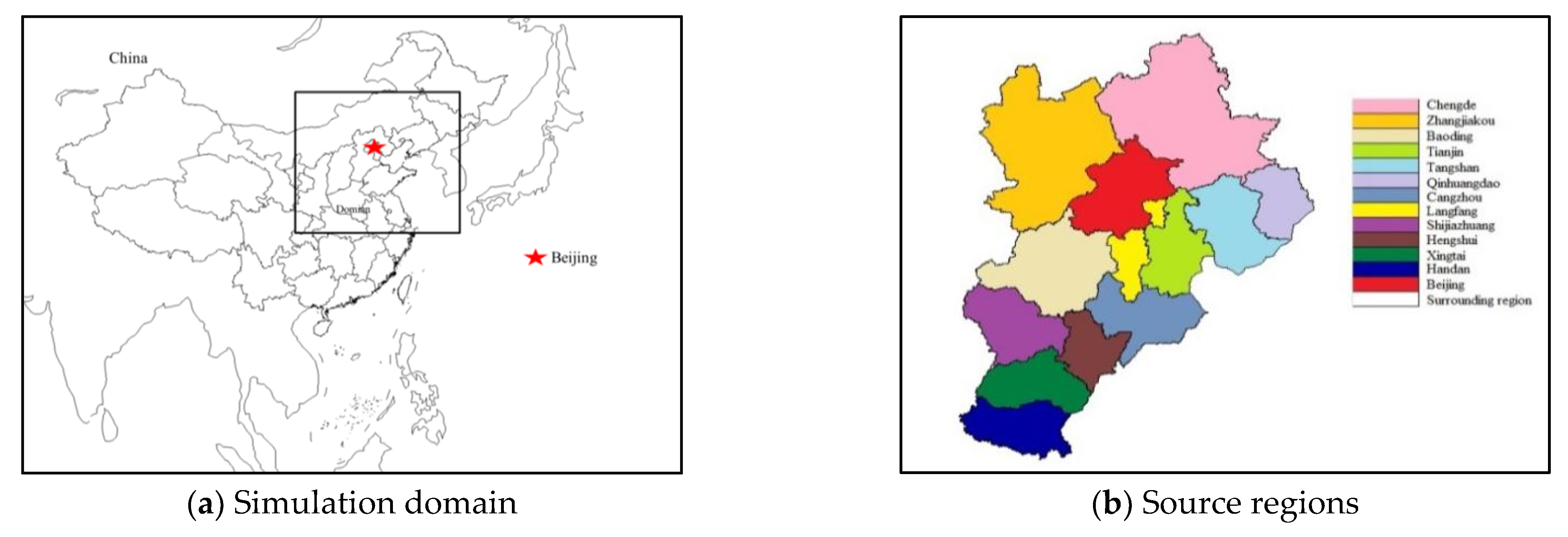
2.1. Model Description and Configuration

Meteorological conditions were simulated by employing the Weather Research and Forecasting (WRF) model (Version 3.4) [27]. The initial meteorological data and boundary conditions were derived from the National Centers for Environmental Prediction (NECP) Final Analysis reanalysis data. The New Thompson, Goddard short-wave, rapid radiative transport model long-wave, Yonsei University planetary boundary layer meteorology, Noah land surface model, and New Grell schemes were selected for the simulation. The CAMx model, version 6.0, was used to study the source apportionment in this study. CAMx is a kind of Eulerian photochemical dispersion model that allows comprehensive “one-atmosphere” assessments of air pollution to be conducted over spatial scales from neighborhoods to continents. The CAMx model is an offline 3D chemical transport model. In this work, the Carbon Bond 2005 (CB05) mechanism was used for the gas-phase chemistry [28]. The aerosol chemistry scheme was chosen from the Regional Acid Deposition Model (RADM-AQ) [29]. The piecewise parabolic method (PPM) and Euler backward iterative (EBI) solvers were applied to the horizontal advection solution options and gas-phase chemistry solver options, respectively. Different PM2.5 components, such as NO3; SO42; secondary organic aerosols (SOAs); primary PM (primary organic aerosols, elemental carbon, crustal fine, crustal coarse, and other coarse particles); and O3, can be distributed in the PSAT module of CAMx. PSAT has been universally applied for source apportionment studies [30,31].
The coverage area of the WRF/CAMX model was a portion of Northern China. The horizontal resolution was 9 km, divided into 220 × 200 horizontal grid cells (as shown in Figure 1a). The modeling vertical resolution was divided into thirty logarithmic structure layers. These layers ranged from the surface to a fixed pressure of 100 mb. The base emission inventory input in the study used the 0.25° Multiresolution Emission Inventory for China (MEIC) of 2016 (http://meicmodel.org, accessed on 15 March 2020). The MEIC included five categories of sources (i.e., industry, traffic, residential, power, and agriculture).

2.2. Simulation Design

PSAT is a species tagging method that marks source regions and emission categories based on the pollutants of interest designed by the user. Beijing was selected as the receptor region. The grid cell at the center of the city was regarded as the receptor. Five emission source categories and 13 source region emission groups were considered in the model. The five emission categories were labeled industry, traffic, residential, power, and agriculture. The entire domain was divided into 13 source regions: Beijing, Tianjin, Baoding, Tangshan, Langfang, Zhangjiakou, Chengde, Cangzhou, Shijiazhuang, Qinhuangdao, Hengshui, Xingtai, and Handan. The source regions were defined based on their geographical borders (shown in Figure 1b). The model simulation was applied for January and July of 2016 with the corresponding meteorological conditions. The month of January was chosen to represent the winter, and July was chosen to represent the summer. The emissions were based on the emission inventory of 2016. Regional sensitivity coefficients were examined based on the CAMx/PSAT simulation. Here, the same pollutant emissions were set in each simulation grid. The regional contributions to air pollution in Beijing were designed to represent the regional sensitivity coefficients. Table 1 summarizes the configurations of the model sensitivity simulation.

2.3. Model Performance

The results of the WRF model simulation were evaluated by data from the Meteorological Information Comprehensive Analysis and Process System (MICAPS), China’s meteorological observation network. The simulation results of the air quality were evaluated by monitoring the air pollutant concentrations collected from the China National Environmental Monitoring Center (CNEMC). The CNEMC website (http://106.37.208.228:8082/, accessed on 15 August 2020) releases hourly air quality information for 367 monitored cities in China. The CNEMC website was also used for studying the spatial and temporal variations of air pollutant concentrations. The meteorological simulation results and air quality concentrations from Run 1 and Run 3 were evaluated. This research used the correlation coefficient (RC), normalized mean bias (NMB), and normalized mean gross error (NME) for the statistical analysis, according to the US Environmental Protection Agency (EPA) model evaluation protocol [32] and previous studies [33]. The surface PM2.5 concentrations, O3 concentrations, NO2 concentrations, and SO2 concentrations were determined by comparing the simulated results with the CNEMC monitoring data. The temperature at 2 m, wind speed at 10 m, and relative humidity (RH) at 2 m were compared with the MICAPS monitoring data. The evaluation statistics of the meteorological and air quality results in the winter and summer of 2016 are summarized in Table 2.
Figure 2a displays the daily simulated and monitored meteorological variables. The results of the meteorological variables—namely, the temperature at 2 m (T2), wind speed at 10 m (WS10), and relative humidity at 2 m (RH2), were verified. The WRF simulation results adequately captured the variations in T2 for each month, with RC values of 0.96 and 0.83 in the winter and summer, respectively. The NMB and NME also indicated an excellent model performance for T2. The NMB value of T2 was −0.22% in the winter and 0.52% in the summer. In the winter and summer, the NME values of T2 were 0.38% and 0.56%, respectively. The WRF simulation results fully reflected the change in wind speed, with average bias values of 16.92% and 46.44% in the winter and summer simulation periods, respectively. The RC of wind speed was 0.84 and 0.66, and the NME was 28.01% and 48.08% in the winter and summer, respectively. As shown in Table 2, the results showed small NMB values for the RH2 simulation of 6.58% in the winter and −11.98% in the summer. The RH2 simulation results had good RC results of 0.88 and 0.77 in the winter and summer, respectively. Table 2 also summarizes the statistics for the PM2.5, SO2, NO2, and O3 concentrations in the two seasons in Beijing. Figure 2b presents the daily simulated and observed results of the PM2.5, SO2, NO2, and O3 concentrations. In the winter, the NMB values for the results of the PM2.5, SO2, NO2, and O3 concentrations were 42.43%, 72.71%, 2.41%, and 28.93%, respectively. In the summer, the NMB values for the results of the PM2.5, SO2, NO2, and O3 concentrations were 10.71%, 38.75%, −10.69%, and −24.74%, respectively. The NME values of the PM2.5, SO2, NO2, and O3 concentrations obtained from the simulation were 63.96%, 80.51%, 32.96%, and 32.68% in the winter, respectively. The NME values of the PM2.5, SO2, NO2, and O3 concentrations obtained from the simulation were 38.83%, 48.81%, 17.05%, and 36.18% in the summer, respectively. These biases may be due to the following reasons. (1) A previous study showed that the uncertainty of 0.25° in the MEIC at some sites would influence the accuracy of the simulation results. (2) The uncertainties related to the meteorological simulation could affect the results. (3) Additionally, the inherent characteristics of the model can lead to a significant deviation in the days of severe pollution. Overall, in this work, the WRF model and CAMx predicted the variables reasonably well. The surface PM2.5, SO2, NO2, and O3 concentrations were well-reproduced by the model. The RC values of the PM2.5, SO2, and NO2 concentrations between the simulated and observed values were between 0.52 and 0.73. The model simulation results (shown in Figure 2) effectively represented the regional pollution processes. All the simulation parameters in our study followed the guidelines of the U.S. EPA. The CAMx results could be used for the further simulation analysis of sensitivity source apportionment.

3. Results and Discussion

3.1. Spatial–Temporal Variations of Air Pollution and Meteorological Factors

Figure 3 presents the temporal variations of the hourly PM2.5, SO2, and NO2 concentrations in Beijing during January and July of 2016. In addition, the hourly wind speed, wind direction, planetary boundary layer height (PBLH), and humidity are also presented at the bottom and top of Figure 3. We found that the hourly variations of the SO2 and NO2 concentrations agreed with the PM2.5 variations, indicating that they might have originated from the same emission pollution sources. The PM2.5, SO2, and NO2 concentrations were negatively correlated with the wind speed. The higher the wind speed was, the smaller the air pollutant concentration. The wind speed contributed to the dispersion of air pollutants out of the region. The air pollutant concentrations were negatively correlated with the PBLH. The higher the PBLH was, the better the dispersion of air pollution. Additionally, the air pollutant concentrations were positively correlated with the RH at 2 m. The higher the humidity was, the more serious the pollution. A higher humidity favored the PM2.5 precursors (i.e., SO2, NOx, NH3, and VOCs) and tended to form PM2.5 through chemical reactions [34]. The higher the humidity was, the lower the PBLH and wind speed, and the more serious the pollution. The transformation and physical diffusion of air pollutants were affected mainly by the wind speed, wind direction, RH2, and PBLH. The higher the wind speed was, the better the diffusion of the air pollutants, and different wind directions led to divergences in terms of the transport of different pollution concentrations. The wind directions in Figure 3 show that the high concentration of air pollutants persisted under the condition of southerly winds, which was conducive to the transport of air pollutants from the surrounding areas to Beijing. The emission levels of Baoding and Shijiazhuang, which are located to the southwest of Beijing, were relatively high. The continuous transport of pollutants could lead to an increase in the PM2.5 level. Previous studies also showed a pollution transport channel in Southwestern Beijing [35]. In addition to the ground observation data, the satellite observation data were also used to present the spatial distribution of regional pollution. Data products on air pollutants retrieved by satellite were from the Ozone Monitoring Instrument (OMI) aboard the National Aeronautics and Space Administration (NASA) satellite Aura (https://disc.sci.gsfc.nasa.gov/, accessed on 15 July 2021) [36]. The downloaded dataset was in HDF5 format and drawn into visual graphics by NCL software. Spatial distributions based on satellite observation results of NO2 concentrations near the ground in January and July 2016 were shown Figure 4. Compared with the winter, the pollution situation slowed down in the summer. The spatial distributions of NO2 pollution were also consistent in the whole process. Heavy air pollution originated from the southern part of the BTH region and spread toward the northern parts, accumulating in front of the Yanshan Mountains and Taihang Mountains in the western and northern domains, respectively. The cities of Shijiazhuang, Baoding, and Beijing and the southern parts of the BTH region experienced heavy air pollution.
The masses of SO42, NO3, and NH4+ aerosols accounted for the largest proportion in PM2.5, especially under pollution conditions. In this work, the various tendencies of SNA in PM2.5 from the simulation results for January and July were calculated, as shown in Figure 5. The SNA simulation results were also compared with monitoring data from a previous study conducted by our group [37]. In January, the mean observed SNA concentration was 30 μg m3, and the mean simulated SNA concentration was 21 μg m3. The observation results showed that SO42, NO3, and NH4+ accounted for 34%, 36%, and 30% of the total SNA, respectively, while the simulation results showed that SO42, NO3, and NH4+ accounted for 36%, 38%, and 26%, respectively. In the summer, the mean observed SNA concentration was 35 μg m3, and the mean simulated SNA concentration was 26 μg m3. The observation results showed that SO42, NO3, and NH4+ accounted for 32%, 36%, and 32% of the total SNA, respectively, while the simulation results showed that SO42, NO3, and NH4+ accounted for 36%, 37%, and 27%, respectively. Nitrate accounted for the most significant proportion of SNA in both the winter and summer.

3.2. Source Apportionment of PM2.5

In this work, the analyses of the total PM2.5 concentration; SO42; NO3−; NH4+; and their precursor gases (SO2, NO2, and NH3) were performed by the CAMx-PSAT model. The sources were separated into five categories: industry, traffic, residential, power, and agriculture. Figure 6 shows the results of the source apportionment for the total PM2.5 concentration. The results suggest that residents became a primary source of pollution in the winter in Beijing (as shown in Figure 6a). The sharp increase in emissions from residential sources in the winter was attributed to the large amount of coal consumed for heating purposes in cold weather. Residential sources contributed 50 μg m−3 to the PM2.5 concentration in January, comprising 38 μg m−3 from local emissions and 12 μg m−3 from regional transport. Industry became the second-largest source, contributing 24 μg m−3 to the PM2.5 concentration, comprising 16 μg m−3 from local emissions and 8 μg m−3 from regional transport. Traffic emissions contributed 13 μg m−3 to the PM2.5 concentration and were mostly from local vehicle contributions (11 μg m−3 from local emissions). Agriculture and power emissions contributed 4.4 μg m−3 and 2.1 μg m−3, respectively. Agricultural sources mainly emitted NH3, which is an important precursor to PM2.5 formation. The replacement of clean energy such as natural gas and the application of pipe end control technology in power plants, reduced the emissions of PM2.5, SO2, and NOx to very small levels [5]. Especially in Beijing, all coal-fired power plants have been shut down. Therefore, the local power emissions contributed only less than 1% to the PM2.5 concentration. The emissions from residents, the industry, traffic, agriculture, and power accounted for 54%, 25%, 14%, 5%, and 2% of PM2.5, respectively. The monthly transport ratio of PM2.5 was 27%. The regional transport of residential and industrial emissions contributed the most, accounting for 13% and 9% of the PM2.5 concentration, respectively. In this work, the results of source apportionment were compared with those of previous studies. Li et al. [38] utilized the CAMx model to make predictions that the industry and residential sectors played a leading role in the PM2.5 concentration in Beijing from 2006 to 2013 in the winter, with residential sources contributing the most (~50%), followed by the industry (~30%). According to a PMF model, Yu et al. [21] found that coal combustion and industrial emissions were the primary sources of PM2.5 in the winter of 2016 in Beijing, accounting for 50% and 27%, respectively. Figure 6b presents the results of the source apportionment for the total PM2.5 concentration in the summer. The results show that industrial emissions were a major pollution source in the summer in Beijing. Industrial sources contributed 35 μg m−3 to the PM2.5 concentration, comprising 13 μg m−3 from local emissions and 22 μg m−3 from regional transport. Traffic was the second-largest source, contributing 20 μg m−3 to the PM2.5 concentration, comprising 16 μg m−3 from local emissions and 4 μg m−3 from regional transport. Residential emissions contributed 17 μg m−3 to the PM2.5 concentration, including 10 μg m−3 from local emissions. The emissions from the industry, traffic, residents, agriculture, and power accounted for 42%, 24%, 20%, 10%, and 4% of PM2.5, respectively. The monthly transport ratio of PM2.5 was 46%. The regional transport of industrial emissions contributed the most in the summer.

3.3. Source Apportionment of Secondary Inorganic Components and Their Precursor Gases

Figure 7a,b shows the source apportionment results for SO42 and its precursor gas SO2. SO42 and SO2 were mainly contributed by industrial and residential emissions. In the winter, the emissions from residents, industry, traffic, agriculture, and power contributed 47%, 39%, 10%, 0%, and 4% to the SO42 concentration, respectively. Residential sources contributed 32% of the SO42 concentration from local emissions and 15% from regional transport. The industry contributed 17% of the SO42 concentration from local emissions and 22% from regional transport. In the summer, the emissions from the industry, power, residents, traffic, and agriculture contributed 66%, 13%, 15%, 6%, and 0% to the SO42 concentration, respectively. Industrial sources contributed 9% of the SO42 concentration from local emissions and 57% from regional transport. In the winter, the emissions from residents, industry, traffic, agriculture, and power contributed 42%, 41%, 15%, 0%, and 2% to the SO2 concentration, respectively. Residential sources contributed 35% of the SO2 concentration from local emissions and 7% from regional transport. In the summer, the SO2 concentration was mainly from industrial emissions, comprising 19% from local emissions and 36% from regional transport. The regional transport contribution ratios of SO42 and SO2 were very different, which had a large impact on the SO42− concentration. The reason lies in that, different meteorological conditions not only affect the diffusion of pollutants but also affect the formation process. The regional transport ratios of SO42 were 42% and 74% of the total concentrations in the winter and summer, respectively. In contrast, the regional transport ratios were 18% (82% by local emissions) and 45% (55% by local emissions) of the total SO2 concentration in the winter and summer, respectively. Compared with the contribution of local emissions, the contribution of regional transport was smaller.
The source apportionment results for NO3 and its precursor gas NO2 are shown in Figure 7c,d. NO3 and NO2 were mainly contributed by industrial and traffic emissions. In the winter, the emissions from the residents, industry, traffic, agriculture, and power contributed 15%, 40%, 30%, 0%, and 15% to the NO3 concentration, respectively. Residential sources contributed 9% of the NO3 concentration from local emissions and 6% from regional transport. The industry contributed 15% from local emissions and 25% from regional transport. Traffic contributed 15% to the NO3 concentration from local emissions and 15% from regional transport. The emissions from residents, industry, traffic, agriculture, and power contributed 14%, 37%, 42%, 0%, and 7% to the NO2 concentration, respectively. Residential sources contributed 12% to the NO2 concentration from local emissions and 2% from regional transport. The industry contributed 30% of the NO2 concentration from local emissions and 7% from regional transport. Traffic contributed 37% of the NO2 concentration from local emissions and 5% from regional transport. In the summer, the emissions from the industry, traffic, power, and residents contributed 49%, 34%, 15%, and 2% to the NO3 concentration, respectively. Industrial sources contributed 9% of the NO3 concentration from local emissions and 40% from regional transport. Traffic contributed 11% to the NO3- concentration from local emissions and 23% from regional transport. The emissions from traffic, industry, power, and residents contributed 53%, 35%, 9%, and 3% to the NO2 concentration, respectively. Traffic contributed 42% to the NO2 concentration from local emission sources and 11% from regional transport. Similar to the results for SO42, regional transport also had a significant effect on the NO3 concentration, accounting for 59% and 75% of the total concentration in the winter and summer, respectively. As SO42 and NO3 are both secondary pollutants, their formation processes are relatively complex, and they are mainly rich in small particles, which are conducive to being transported over long distances. In contrast, regional transport accounts for 16% of the total NO2 concentration in the winter and 32% in the summer. Compared with the contribution from regional transport, local emissions have more significant contributions to the NO2 concentration. Among the local emissions, traffic emissions contributed most to the total NO2 concentration. NH4+ and NH3 were mainly contributed by agricultural emissions, which accounted for 94% of the total NH4+ concentration and 95% of the NH3 concentration. A previous study also found that agricultural sources contribute to most ammonia emissions [39]. Residential and traffic emissions accounted for less than 6% of the total NH4+ concentration and less than 4% of the NH3 concentration. Compared with the contribution from local emissions, regional transport contributed less. Local emissions contributed approximately 80% of the NH4+ concentration in Beijing in the two seasons.

3.4. Source Apportionment of O3

Figure 8 shows the source contributions and regional transport concentrations of the winter and summer monthly average O3 concentrations. Industry and transportation sources were the two major emission sectors contributing to O3 pollution in Beijing (as shown in Figure 8a). In the winter, the emissions from the industry, traffic, residents, power, and agriculture contributed 36%, 43%, 17%, 4%, and 0% to the O3 concentration, respectively. In the summer, the emissions from the industry, traffic, residents, power, and agriculture contributed 49%, 38%, 7%, 6%, and 0% to the O3 concentration, respectively. These results are generally consistent with the source apportionment results for NO2 shown in Figure 7. Wang et al. [26] similarly discovered that industrial and traffic emissions were the main sources of O3 in the summer in Beijing, accounting for 38% and 22%, respectively. The monthly transport ratio of O3 was 31% and 65% in the winter and summer, respectively. Regional transport contributed the most in the summer. In the winter, industrial sources contributed 15% of the O3 concentration from local emissions and 21% from regional transport. Traffic contributed 37% to the O3 concentration from local emissions and 6% from regional transport. In the summer, industrial sources contributed 13% of the O3 concentration from local emissions and 36% from regional transport. Traffic contributed 16% to the O3 concentration from local emissions and 22% from regional transport. Liu et al. [40] found that, during an O3 pollution episode in Beijing, the local emissions contributed 14% to the O3 concentration. It has been proven that high concentrations of O3 pollution are derived not only from local emissions but also from regional transport and even superregional transport. Figure 8b shows the regional transport source apportionment results for the O3 concentration. Zhangjiakou was found to be the central transport region for Beijing O3 pollution in the winter, and the transport contribution ratio to PM2.5 was 27%. In the summer, Langfang, Tianjin, Tangshan, and Baoding were the major transport regions, with transport contribution ratios to O3 of 10%, 10%, 8%, and 8%, respectively. As Derwent et al. [41] reported, O3 can be transported thousands of kilometers in the atmosphere and can persist for long periods of time in the troposphere. Although Shijiazhuang, Hengshui, Handan, and Xingtai are far from Beijing, their emission contributions to O3 pollution in Beijing were prominent, accounting for 5%, 5%, 4%, and 3% in the summer, respectively. These results show that regional collaboration is an important and necessary prerequisite for controlling O3 pollution in Beijing.

3.5. Regional Sensitivity Coefficient Results

To better understand how the topography and meteorology affect Beijing’s air pollution, the regional sensitivity coefficients were examined based on the CAMx/PSAT simulation. The sensitivity coefficients of the air pollutants for different regions in the winter and summer were obtained. The same pollutant emissions were set in each simulation grid, as described in Section 2.2. The results show that local emissions were the major sensitive area of pollution formation in the winter. In the winter, the regional sensitivity coefficients of PM2.5, SO42, and NO3 were 57%, 50%, and 60%, respectively. In the summer, the regional sensitivity coefficients of PM2.5, SO42, and NO3 were 43%, 26%, and 50%, respectively. These results illustrate that, in pollution control, more attention should be paid to local emission sources first, followed by the coordinated control of regional sources. Compared with SO42 and NO3, the local region of Beijing was more sensitive to their precursor gases. The regional sensitivity coefficients of SO2 and NO2 were 64% and 82% in the winter, respectively, and 56% and 58% in the summer. These results further confirmed that the contribution of regional transport had a more significant impact on the secondary inorganic aerosol concentrations than on the concentrations of their precursor gases. To clearly understand the region’s sensitivity in generating air pollution, the sensitivity coefficients of the surrounding cities are shown in Figure 9. The results are divided into four levels: strong sensitivity, general sensitivity, weaker sensitivity, and insensitivity. In the winter, the sensitivity coefficients of Zhangjiakou, Chengde, and Langfang were more significant than those of the other cities. Zhangjiakou, Chengde, and Langfang, the regions characterized by strong sensitivity, are very close to Beijing (northwest, northeast, and south of Beijing, respectively). According to the meteorological records, northwesterly, northerly, and northeasterly wind directions were frequently observed in Beijing in January 2016 (as shown in Figure 10). Zhangjiakou and Chengde were located upwind of Beijing. The cities of Baoding, Tianjin, and Tangshan were characterized by a general sensitivity, while the cities of Cangzhou, Qinhuangdao, and Hengshui were characterized by a weaker sensitivity. Finally, due to their large distances from Beijing, the cities of Shijiazhuang, Handan, and Xingtai were characterized as insensitive to the air pollution in Beijing. In the summer of 2016, the southwesterly and northeasterly wind directions frequently occurred in Beijing. In this case, Langfang, Tianjin, Tangshan, and Baoding were the regions with strong sensitivity. As Zhangjiakou is downwind of Beijing in the summer, this city was insensitive.
Figure 11 shows the high-resolution regional source apportionment results. It was found that Langfang, Baoding, Tangshan, and Zhangjiakou were the major transport regions for Beijing air pollution in the winter, and the transport contribution ratios to PM2.5 were 8%, 5%, 4%, and 4%, respectively. The contributions to the PM2.5 concentration from Tianjin, Cangzhou, Chengde, Qinhuangdao, Shijiazhuang, and Hengshui were 1% to approximately 2%. In the summer, Langfang, Tangshan, Tianjin, and Baoding were the major transport regions for Beijing’s PM2.5 pollution, and the transport contribution ratios to PM2.5 were 14%, 10%, 8%, and 5%, respectively. Since there were few northwest winds in the summer of 2016, Zhangjiakou’s emission contribution was close to 0%. Comparing the regional sensitivity coefficients shown in Figure 9, the long-distance transport of pollution was increased. For example, the contributions from the cities of Shijiazhuang and Hengshui were more prominent, and even emissions from Xingtai impacted the air pollution in Beijing. The PM2.5, SO2, and NOx emission inventories released by the MEIC are given in Table 3 [42]. It is clearly shown that Tangshan and Baoding had high pollutant emissions. These cities have always been greatly affected and challenged by coal burning and the iron manufacturing industry due to their rapid economic development. By contrast, the pollutant emissions from Zhangjiakou and Chengde were relatively small. Therefore, to make considerable progress in improving the air quality of Beijing, regional control measures should be a priority and should focus on the regions with large emission contributions (i.e., Tangshan, Baoding, Langfang, and Tianjin). When discussing the development of the economy and improving the air quality, pollution emission sources cannot be newly added and arranged in sensitive regions (i.e., Zhangjiakou, Chengde, and Langfang).
Nevertheless, some uncertainties and limitations might bring the effect on the research results. Although CAMx-PSAT has been developed to quantify the source of air pollution and evaluate their contributions, which is affected by the uncertainties in terms of the meteorology simulations, parameterizations, and formulations used in the model. As for the MEIC, it is a bottom-up emission inventory model gradually developed for China. The limitations of research on the discharge coefficient, activity rates, and emission reductions measures would lead to uncertainties in the judgment of emission tendencies [43]. New chemical mechanism and more accurate emission inventory are needed to be the focus of future research.

4. Conclusions

The CAMx-PSAT model was employed in this work for the high-spatial resolution source apportionment of SNA in PM2.5, their corresponding precursor gases, and O3 in the winter and summer over Beijing. Both the contributions of different source categories of emissions and detailed information on regional transport were obtained. The regional sensitivity coefficients were also calculated and were introduced to express the impact of regional topography and meteorology on the Beijing air quality. The meteorological and air quality simulation concentrations were verified by observational data. The simulation results were in acceptable agreement with the observed data. The WRF-CAMx model showed an outstanding performance in representing the meteorological and air pollution processes.
We found that the higher the humidity was, the lower the PBLH and wind speed, and the more serious the PM2.5 pollution. The results also showed that southerly winds favored the transport of air pollutants from the surrounding regions to Beijing. In the winter, the emissions from the residents, industry, traffic, agriculture, and power accounted for 54%, 25%, 14%, 5%, and 2% of PM2.5, respectively. In the summer, the emissions from the industry, traffic, residents, agriculture, and power accounted for 42%, 24%, 20%, 10%, and 4% of PM2.5, respectively. The monthly transport ratios of PM2.5 were 27% and 46% in the two seasons, respectively. The regional transport of residential and industrial emissions contributed the most. For local emission, a leading source of pollution in Beijing in the summer came from local traffic emissions. SO42− and SO2 were mainly contributed by industrial and residential emissions. Industrial and traffic emissions mainly contributed to the concentrations of NO3 and NO2. Regional transport also had a significant effect on the SO42− and NO3 concentrations. Local emissions were the main source of SO2 and NO2 pollution. Northwesterly, northerly, and northeasterly winds frequently occurred in Beijing in the winter, and thus, Zhangjiakou, Chengde, and Langfang were the regions with strong sensitivity to the formation of air pollution over Beijing. In the summer, southwesterly and northeasterly winds were frequent in Beijing; as a result, Langfang, Tianjin, Tangshan, and Baoding were the regions with strong sensitivity.
Industries and traffic sources were the two major emission sectors that contributed to O3 pollution in Beijing. This study also showed that O3 pollution was derived from local emissions and regional transport. The monthly transport ratios of O3 were 31% and 65% in the winter and summer, respectively. Zhangjiakou was the central transport region for Beijing O3 pollution in the winter, whereas Langfang, Tianjin, Tangshan, and Baoding were the major transport regions for pollution in the summer. It is necessary to focus on regional collaboration to control both the local and nearby area emission sources.

Author Contributions

Experimental design and manuscript writing, W.W. and X.M.; supervision and critical comments, Y.X. and W.S.; data collection and result analysis, S.S., J.W., Y.W. and L.L. All authors have read and agreed to the published version of the manuscript.

Funding

This research was supported by the National Natural Science Foundation of China (Grant Nos. 51808549 and 21806183), Basic Research Fund of CAMS (2020Z002).

Institutional Review Board Statement

Not applicable.

Informed Consent Statement

Not applicable.

Conflicts of Interest

The authors declared that they have no conflict of interest in this work.

References

  1. Ma, Y.; Xin, J.; Zhang, W.; Liu, Z.; Ma, Y.; Kong, L.; Wang, Y.; Deng, Y.; Lin, S.; He, Z. Long-term variations of the PM2.5 concentration identified by MODIS in the tropical rain forest. Southeast Asia. Atmos. Res. 2019, 219, 140–152. [Google Scholar] [CrossRef]
  2. Song, C.; Wu, L.; Xie, Y.; He, J.; Chen, X.; Wang, T.; Lin, Y.; Jin, T.; Wang, A.; Liu, Y.; et al. Air pollution in China: Status and spatiotemporal variations. Environ. Pollut. 2017, 227, 334–347. [Google Scholar] [CrossRef]
  3. Wang, T.; Xue, L.; Brimblecombe, P.; Lam, Y.F.; Li, L.; Zhang, L. Ozone pollution in China: A review of concentrations, meteorological influences, chemical precursors, and effects. Sci. Total Environ. 2017, 575, 1582–1596. [Google Scholar] [CrossRef]
  4. Lang, J.; Cheng, S.; Li, J.; Chen, D.; Zhou, Y.; Wei, X.; Han, L.; Wang, H. A Monitoring and Modeling Study to Investigate Regional Transport and Characteristics of PM2.5 Pollution. Aerosol Air Qual. Res. 2013, 13, 943–956. [Google Scholar] [CrossRef] [Green Version]
  5. The United Nation Environment Program: A Review of Air Pollution Control in Beijing: 1998–2013. Available online: www.unep.org/publications (accessed on 15 July 2020).
  6. Wen, W.; Cheng, S.; Chen, X.; Wang, G.; Li, S.; Wang, X.; Liu, X. Impact of emission control on PM2.5 and the chemical composition change in Beijing-Tianjin-Hebei during the APEC summit 2014. Environ. Sci. Pollut. Res. 2015, 23, 4509–4521. [Google Scholar] [CrossRef]
  7. MEP: 2017 Air Pollution Prevention and Management Plan for the Beijing-Tianjin-Hebei Region and Its Surrounding Areas. Available online: http://dqhj.mee.gov.cn/dtxx/201703/t20170323_408663.shtml (accessed on 18 August 2018).
  8. Beijing Municipal Environmental Protection Bureau (BMEPB). Available online: http://www.bjepb.gov.cn/bjhrb/xxgk/jgzn/jgsz/jjgjgszjzz/xcjyc/xwfb/827457/index.html (accessed on 15 October 2020).
  9. Wang, W.-N.; Cheng, T.-H.; Gu, X.-F.; Chen, H.; Guo, H.; Wang, Y.; Bao, F.-W.; Shi, S.-Y.; Xu, B.-R.; Zuo, X.; et al. Assessing Spatial and Temporal Patterns of Observed Ground-Level Ozone in China. Sci. Rep. 2017, 7, 3651. [Google Scholar] [CrossRef]
  10. Liu, H.; Liu, S.; Xue, B.; Lv, Z.; Meng, Z.; Yang, X.; Xue, T.; Yu, Q.; He, K. Ground-level ozone pollution and its health impacts in China. Atmos. Environ. 2018, 173, 223–230. [Google Scholar] [CrossRef]
  11. Zhang, Y.; Zhao, Y.; Li, J.; Wu, Q.; Wang, H.; Du, H.; Yang, W.; Wang, Z.; Zhu, L. Modeling Ozone Source Apportionment and Performing Sensitivity Analysis in Summer on the North China Plain. Atmosphere 2020, 11, 992. [Google Scholar] [CrossRef]
  12. Thurston, G.D.; Spengler, J.D. A quantitative assessment of source contributions to inhalable particulate matter pollution in metropolitan Boston. Atmos. Environ. (1967) 1985, 19, 9–25. [Google Scholar] [CrossRef]
  13. Habre, R.; Coull, B.; Koutrakis, P. Impact of source collinearity in simulated PM2.5 data on the PMF receptor model solution. Atmos. Environ. 2011, 45, 6938–6946. [Google Scholar] [CrossRef]
  14. Park, E.S.; Sullivan, D.W.; Kang, D.H.; Ying, Q.; Spiegelman, C.H. Assessment of mobile source contributions in El Paso by PMF receptor modeling coupled with wind direction analysis. Sci. Total Environ. 2020, 720, 137527. [Google Scholar] [CrossRef] [PubMed]
  15. Yatkin, S.; Gerboles, M.; Belis, C.; Karagulian, F.; Lagler, F.; Barbiere, M.; Borowiak, A. Representativeness of an air quality monitoring station for PM2.5 and source apportionment over a small urban domain. Atmos. Pollut. Res. 2020, 11, 225–233. [Google Scholar] [CrossRef] [PubMed]
  16. Galvão, E.S.; Reis, N.C.; Santos, J.M. The role of receptor models as tools for air quality management: A case study of an industrialized urban region. Environ. Sci. Pollut. Res. 2020, 27, 35918–35929. [Google Scholar] [CrossRef] [PubMed]
  17. Belis, C.; Pernigotti, D.; Pirovano, G.; Favez, O.; Jaffrezo, J.; Kuenen, J.; van der Gon, H.D.; Reizer, M.; Riffault, V.; Alleman, L.; et al. Evaluation of receptor and chemical transport models for PM10 source apportionment. Atmos. Environ. X 2020, 5, 100053. [Google Scholar] [CrossRef]
  18. Burr, M.J.; Zhang, Y. Source apportionment of fine particulate matter over the Eastern U.S. Part I: Source sensitivity simulations using CMAQ with the Brute Force method. Atmos. Pollut. Res. 2011, 2, 300–317. [Google Scholar] [CrossRef] [Green Version]
  19. Ansari, T.; Ojha, N.; Chandrasekar, R.; Balaji, C.; Singh, N.; Gunthe, S.S. Competing impact of anthropogenic emissions and meteorology on the distribution of trace gases over Indian region. J. Atmos. Chem. 2016, 73, 363–380. [Google Scholar] [CrossRef]
  20. Ojha, N.; Sharma, A.; Kumar, M.; Girach, I.; Ansari, T.; Sharma, S.K.; Singh, N.; Pozzer, A.; Gunthe, S.S. On the widespread enhancement in fine particulate matter across the Indo-Gangetic Plain towards winter. Sci. Rep. 2020, 10, 5862. [Google Scholar] [CrossRef] [Green Version]
  21. Yu, S.; Liu, W.; Xu, Y.; Yi, K.; Zhou, M.; Tao, S.; Liu, W. Characteristics and oxidative potential of atmospheric PM2.5 in Beijing: Source apportionment and seasonal variation. Sci. Total Environ. 2019, 650, 277–287. [Google Scholar] [CrossRef] [PubMed]
  22. Song, Y.; Dai, W.; Shao, M.; Liu, Y.; Lu, S.; Kuster, W.; Goldan, P. Comparison of receptor models for source apportionment of volatile organic compounds in Beijing, China. Environ. Pollut. 2008, 156, 174–183. [Google Scholar] [CrossRef]
  23. Zhang, Y.; Li, X.; Nie, T.; Qi, J.; Chen, J.; Wu, Q. Source apportionment of PM2.5 pollution in the central six districts of Beijing, China. J. Clean. Prod. 2018, 174, 661–669. [Google Scholar] [CrossRef]
  24. Gao, J.; Zhu, B.; Xiao, H.; Kang, H.; Hou, X.; Shao, P. A case study of surface ozone source apportionment during a high concentration episode, under frequent shifting wind conditions over the Yangtze River Delta, China. Sci. Total Environ. 2016, 544, 853–863. [Google Scholar] [CrossRef] [PubMed]
  25. Wang, P.; Chen, Y.; Hu, J.; Zhang, H.; Ying, Q. Source apportionment of summertime ozone in China using a source oriented chemical transport model. Atmos. Environ. 2019, 211, 79–90. [Google Scholar] [CrossRef]
  26. Liu, L.; Liu, Y.; Wen, W.; Liang, L.; Ma, X.; Jiao, J.; Guo, K. Source Identification of Trace Elements in PM2.5 at a Rural Site in the North China Plain. Atmosphere 2020, 11, 179. [Google Scholar] [CrossRef] [Green Version]
  27. Skamarock, W.C.; Klemp, J.B.; Dudhia, J.; Gill, D.O.; Barker, D.M.; Duda, M.G.; Huang, X.Y.; Wang, W.; Powers, J.G. Description of the Advanced Research WRF Version 3 (No. NCAR/TN-475+STR); University Corporation for Atmospheric Research: Boulder, CO, USA, 2008. [Google Scholar]
  28. Yarwood, G.; Rao, S.; Yocke, M.; Whitten, G. Updates to the Carbon Bond Chemical Mechanism: CB05. Final Report prepared for US EPA. Available online: http://www.camx.com/publ/pdfs/CB05_Final_Report_120805.pdf (accessed on 15 December 2020).
  29. Chang, J.S.; Brost, R.A.; Isaksen, I.S.A.; Madronich, S.; Middleton, P.; Stockwell, W.; Walcek, C.J. A three-dimensional Eulerian acid deposition model: Physical concepts and formulation. J. Geophys. Res. Space Phys. 1987, 92, 14681–14700. [Google Scholar] [CrossRef]
  30. Fann, N.; Baker, K.R.; Fulcher, C.M. Characterizing the PM2.5-related health benefits of emission reductions for 17 industrial, area and mobile emission sectors across the U.S. Environ. Int. 2012, 49, 141–151. [Google Scholar] [CrossRef] [PubMed]
  31. Zhang, Y.; Wu, S.-Y. Fine Scale Modeling of Agricultural Air Quality over the Southeastern United States Using Two Air Quality Models. Part II. Sensitivity Studies and Policy Implications. Aerosol Air Qual. Res. 2013, 13, 1475–1491. [Google Scholar] [CrossRef] [Green Version]
  32. Michael, G.B.; Eladio, M.K. Insights from the BRAVO study on nesting global models to specify boundary conditions in regional air quality modeling simulations. Atmos Environ. 2006, 40, 574–582. [Google Scholar]
  33. Wang, L.T.; Wei, Z.; Yang, J.; Zhang, Y.; Zhang, F.F.; Su, J.; Meng, C.C.; Zhang, Q. The 2013 severe haze over southern Hebei, China: Model evaluation, source apportionment, and policy implications. Atmos. Chem. Phys. Discuss. 2014, 14, 3151–3173. [Google Scholar] [CrossRef] [Green Version]
  34. Wang, X.; Zhou, Y.; Cheng, S.; Wang, G. Characterization and regional transmission impact of water-soluble ions in PM2.5 during winter in typical cities. China Environ. Sci. 2016, 36, 2289–2296. [Google Scholar]
  35. Wen, W.; Ma, X.; Wei, P.; Cheng, S.; Wang, X.; He, X.; Liu, L. Understanding the Regional Transport Contributions of Primary and Secondary PM2.5 Components over Beijing during a Severe Pollution Episodes. Aerosol Air Qual. Res. 2018, 18, 1720–1733. [Google Scholar] [CrossRef] [Green Version]
  36. Levelt, P.F.; Van Den Oord, G.H.; Dobber, M.R.; Malkki, A.; Visser, H.; De Vries, J.; Stammes, P.; Lundell, J.O.; Saari, H. The ozone monitoring instrument. IEEE Trans. Geosci. Remote 2006, 44, 1093–1101. [Google Scholar] [CrossRef]
  37. Wang, X.; Wei, W.; Cheng, S.; Yao, S.; Zhang, H.; Zhang, C. Characteristics of PM2.5 and SNA components and meteorological factors impact on air pollution through 2013–2017 in Beijing, China. Atmos. Pollut. Res. 2019, 10, 1976–1984. [Google Scholar] [CrossRef]
  38. Li, X.; Zhang, Q.; Zhang, Y.; Zheng, B.; Wang, K.; Chen, Y.; Wallington, T.J.; Han, W.; Shen, W.; Zhang, X.; et al. Source contributions of urban PM2.5 in the Beijing–Tianjin–Hebei region: Changes between 2006 and 2013 and relative impacts of emissions and meteorology. Atmos. Environ. 2015, 123, 229–239. [Google Scholar] [CrossRef] [Green Version]
  39. Ye, Z.; Guo, X.; Cheng, L.; Cheng, S.; Chen, D.; Wang, W.; Liu, B. Reducing PM2.5 and secondary inorganic aerosols by agricultural ammonia emission mitigation within the Beijing-Tianjin-Hebei region, China. Atmos. Environ. 2019, 219, 116989. [Google Scholar] [CrossRef]
  40. Li, L.; Chen, C.H.; Huang, C.; Huang, H.Y.; Zhang, G.F.; Wang, Y.J.; Wang, H.L.; Lou, S.R.; Qiao, L.P.; Zhou, M.; et al. Process analysis of regional ozone formation over the Yangtze River Delta, China using the Community Multi-scale Air Quality modeling system. Atmos. Chem. Phys. Discuss. 2012, 12, 10971–10987. [Google Scholar] [CrossRef] [Green Version]
  41. Derwent, R.; Simmonds, P.; Seuring, S.; Dimmer, C. Observation and interpretation of the seasonal cycles in the surface concentrations of ozone and carbon monoxide at mace head, Ireland from 1990 to 1994. Atmos. Environ. 1998, 32, 145–157. [Google Scholar] [CrossRef]
  42. Tsinghua University. Multi-Resolution Emission Inventory for China. 2016. Available online: http://www.meicmodel.org/ (accessed on 15 March 2020).
  43. Cheng, J.; Su, J.; Cui, T.; Li, X.; Dong, X.; Sun, F.; Yang, Y.; Tong, D.; Zheng, Y.; Li, Y.; et al. Dominant Role of Emission Reduction in PM2.5 Air Quality Improvement in Beijing during 2013–2017: A Model-based Decomposition Analysis. Atmos. Chem. Phys. 2019, 19, 6125–6146. [Google Scholar] [CrossRef] [Green Version]
Figure 1. Model simulation domain and source regions.
Remotesensing 13 03457 g001
Figure 2. Comparison of the simulated results with the observed data.
Remotesensing 13 03457 g002aRemotesensing 13 03457 g002b
Figure 3. Hourly air quality concentrations and meteorological parameters in the region.
Remotesensing 13 03457 g003
Figure 4. Spatial distributions based on satellite observation results of NO2 concentration in January and July 2016 (molecular/cm2: the number of NO2 molecules per square centimeter).
Remotesensing 13 03457 g004
Figure 5. SNA concentrations in Beijing (Obs: observation; Sim: simulation). (a) the SNA concentrations in winter, (b) the SNA concentrations in summer.
Remotesensing 13 03457 g005
Figure 6. Source apportionment results for PM2.5. (AG: agriculture, PO: power, RE: residential, and Tr: traffic. In the industry, local: local emissions and Tran: transport from the surrounding region). (a) the source apportionment results for PM2.5 in winter, (b) the source apportionment results for PM2.5 in summer.
Remotesensing 13 03457 g006aRemotesensing 13 03457 g006b
Figure 7. Source apportionment results for SNA and its precursor gases. (a) the SO42− source apportionment results, (b) the SO2 source apportionment results, (c) the NO3 source apportionment results, (d) the NO2 source apportionment results.
Remotesensing 13 03457 g007
Figure 8. Source apportionment results for O3. (a) the O3 source apportionment results, (b) the region contribution to O3.
Remotesensing 13 03457 g008
Figure 9. Regional sensitivity coefficients for Beijing.
Remotesensing 13 03457 g009
Figure 10. Distributions of wind directions in January and July 2016. (a) the distributions of wind directions in January, (b) the distributions of wind directions in July.
Remotesensing 13 03457 g010
Figure 11. High-resolution source apportionment results.
Remotesensing 13 03457 g011
Table 1. Simulation design.
SimulationMonthCategories of SourcesSource RegionsEmissions
Run 1JanuaryIndustry, traffic, residential, power, agriculture13Real emission inventory of January 2016
Run 2JanuaryIndustry, traffic, residential, power, agriculture13Same pollutant emissions in each grid cell
Run 3JulyIndustry, traffic, residential, power, agriculture13Real emission inventory of July 2016
Run 4JulyIndustry, traffic, residential, power, agriculture13Same pollutant emissions in each grid cell
Table 2. The statistical results of the simulated and monitored data in Beijing.
SimulationObservationNMB (%)NME (%)RC
WRFT2 (K)—winter268.33268.91−0.220.380.96
WS10 (m s−1)—winter2.812.4016.9228.010.84
RH2 (%)—winter39.5037.046.5814.30.88
T2 (K)—summer302.25300.690.520.560.83
WS10 (m s−1)—summer2.942.0146.4448.080.66
RH2 (%)—summer61.0669.37−11.9815.340.77
CAMxPM2.5 (μg m−3)—winter94.7266.5042.4363.960.73
SO2 (μg m−3)—winter34.7220.1172.7180.510.72
NO2 (μg m−3)—winter52.9550.802.4132.960.52
O3 (μg m−3)—winter55.8043.1328.9332.680.52
PM2.5 (μg m−3)—summer84.0075.8810.7138.830.78
SO2 (μg m−3)—summer5.143.7038.7548.810.52
NO2 (μg m−3)—summer30.0733.67−10.6917.050.55
O3 (μg m−3)—summer122.15162.3−24.7436.180.61
Table 3. Emission inventory in the Beijing–Tianjin–Baoding region (ton/year).
SO2NOxPM2.5
Tangshan193,593351,055104,186
Shijiazhuang137,704275,64483,467
Tianjin121,170328,15865,259
Handan100,533189,70263,110
Baoding96,388195,79071,567
Cangzhou87,703172,00457,502
Xingtai66,736124,69545,135
Langfang49,502113,53335,905
Hengshui45,04387,24732,175
Zhangjiakou44,11292,11930,051
Chengde39,66773,20727,239
Beijing33,068224,45153,052
Qinhuangdao31,80266,84120,516
Publisher’s Note: MDPI stays neutral with regard to jurisdictional claims in published maps and institutional affiliations.

