Abstract
The Earth’s time-variable gravity field is of great significance to study mass change within the Earth’s system. Since 2002, the NASA-DLR Gravity Recovery and Climate Experiment (GRACE) and its successor GRACE follow-on mission provide observations of monthly changes in the Earth gravity field with unprecedented accuracy and resolution by employing low-low satellite-to-satellite tracking (LLSST) measurements. In addition to LLSST, monthly gravity field models can be acquired from satellite laser ranging (SLR) and high-low satellite-to-satellite tracking (HLSST). The monthly gravity field solutions HLSST+SLR were derived by combining HLSST observations of low earth orbiting (LEO) satellites with SLR observations of geodetic satellites. Bandpass filtering was applied to the harmonic coefficients of HLSST+SLR solutions to reduce noise. In this study, we analyzed the performance of the monthly HLSST+SLR solutions in the spectral and spatial domains. The results show that: (1) the accuracies of HLSST+SLR solutions are comparable to those from GRACE for coefficients below degree 10, and significantly improved compared to those of SLR-only and HLSST-only solutions; (2) the effective spatial resolution could reach 1000 km, corresponding to the spherical harmonic coefficient degree 20, which is higher than that of the HLSST-only solutions. Compared with the GRACE solutions, the global mass redistribution features and magnitudes can be well identified from HLSST+SLR solutions at the spatial resolution of 1000 km, although with much noise. In the applications of regional mass recovery, the seasonal variations over the Amazon Basin and the long-term trend over Greenland derived from HLSST+SLR solutions truncated to degree 20 agree well with those from GRACE solutions without truncation, and the RMS of mass variations is 282 Gt over the Amazon Basin and 192 Gt in Greenland. We conclude that HLSST+SLR can be an alternative option to estimate temporal changes in the Earth gravity field, although with far less spatial resolution and lower accuracy than that offered by GRACE. This approach can monitor the large-scale mass transport during the data gaps between the GRACE and the GRACE follow-on missions.
1. Introduction
The time-variable Earth gravity field provides information about mass redistributions within the Earth system, which allows studying temporal changes in terrestrial water storage associated with changes in terrestrial hydrology (soil moisture and groundwater) and the mass balance of glaciers, sea level rise, and solid Earth movements, e.g., glacial isostatic adjustment (GIA) and earthquakes [1]. The Gravity Recovery and Climate Experiment (GRACE) mission [2,3], launched on March 17, 2002, and its successor, the GRACE Follow-on mission [4], launched on May 22, 2018, determine the monthly global gravity models with a spatial resolution of about 300 km with an accuracy of 2 cm [5] from precise K-band ranging between two satellites separated by 220 km along their orbit track, i.e., employing low-low aatellite-to-satellite (LLSST) measurements. Monthly GRACE LLSST gravity field solutions, e.g., the official GRACE Level-2 products in the form of spherical harmonic coefficients, are provided by three GRACE data processing centers: the Center for Space Research (CSR) at the University of Texas at Austin, Geoforschungszentrum (GFZ) in Potsdam, and NASA Jet Propulsion Laboratory (JPL). Data products and documents are available from either GFZ’s Information System and Data Center (ISDC) [6] or JPL’s Physical Oceanography Distributed Active Archive Center (PO.DAAC) [7]. However, there are short data gaps of up to several months in the GRACE/GRACE follow-on mission lifetime due to data loss during eclipsing periods and orbit resonance, and a long data gap from June 2017 to June 2018 between the GRACE and the GRACE follow-on missions [8,9].
In addition to the GRACE LLSST, there are other methods for obtaining the time-variable Earth gravity field. Satellite laser ranging (SLR) was typically used to recover low-degree coefficients of the time-variable gravity field with high precision [10,11,12,13] before the advent of dedicated gravimetric missions. However, the spatial resolution of SLR is limited due to the high altitude of geodetic SLR satellites and scarce tracking data. Matsuo et al. [14], Sośnica et al. [15], and Cheng [16] recovered the time-variable gravity field using several SLR satellites with coefficients up to degrees 4, 10, and 5, respectively. High-low satellite-to-satellite (HLSST) is another method of obtaining the time-variable Earth gravity field based on precise kinematic orbits of the LEO from GPS tracking data. The Challenging Minisatellite Payload (CHAMP) mission [17] was a dedicated gravimetric mission based on the HLSST concept. Many studies were conducted with the goal of recovering the time-variable gravity field from GPS HLSST data of CHAMP [18], GRACE [19], GOCE [20], Swarm [21,22,23], and a constellation of LEOs [24], resulting in the improved spatial resolution of about 1300–2000 km. This improvement is attributed to the low altitude of LEOs, global coverage of GPS tracking data, high observation density, and improved GPS data processing. However, due to the poor accuracy of GPS observations with respect to GRACE K-band ranging, the HLSST solutions are inferior to the GRACE LLSST solutions.
The very low degrees (up to degree 5) of the time-variable gravity field can be well determined from SLR, whereas HLSST provides monthly solutions with a relative higher spatial resolution. The combination of SLR and HLSST may result in improved solutions over SLR-only and HLSST-only solutions. Moreover, the combination of SLR to multiple geodetic satellites and HLSST to multiple low Earth orbiting satellites (LEOs) does not depend on the use of a specific satellite. If a satellite finishes the operational phase of the mission, the generation of monthly solutions will not be interrupted because many other satellites are operated in the combination. Thus, continuous and uninterrupted solutions can be guaranteed. In this study, we analyzed the combined monthly gravity field based on HLSST and SLR data generated by Weigelt, et al. [25]. The solutions HLSST+SLR are estimated from GPS HLSST data of multiple LEOs and SLR data of multiple geodetic satellites over 13 years (January 2003 to August 2016). We investigated the performance of the HLSST+SLR solutions compared with the GRACE LLSST solutions and the improvement relative to solutions based on SLR-only and HLSST-only data. The analysis was done both in the spectral and spatial domains. The goal of this paper is to evaluate the accuracy and spatial resolution of the monthly solutions HLSST+SLR and investigate the capability of mass transport recovery at that spatial resolution compared with the GRACE LLSST solutions.
The paper is structured as follows. Section 2 briefly introduces the satellites utilized, the solution methodology, and the analysis strategy. In Section 3, the characteristics of the HLSST+SLR coefficients in the spectral domain are discussed, and the capability of monitoring global and regional mass distributions from the HLSST+SLR solutions is studied in the spatial domain. The main conclusions are drawn in Section 4.
2. Materials and Methods
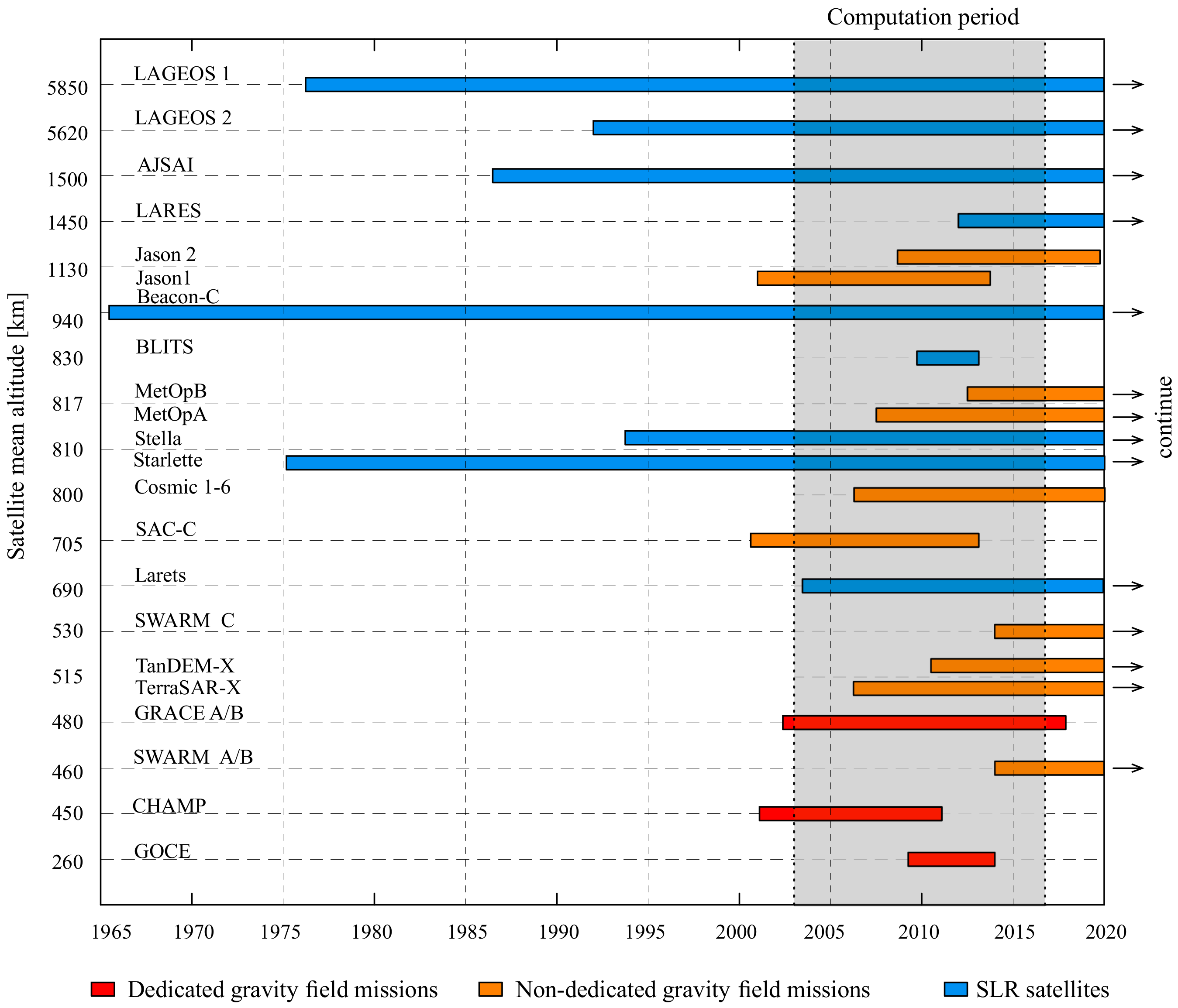
The HLSST and SLR combined solutions are monthly gravity field estimates from Institut für Erdmessung (IfE), Leibniz Universität Hannover, provided as sets of spherical harmonic coefficients up to degree and order 90, spanning from January 2003 to August 2016. A total number of 20 LEO satellites and 9 SLR geodetic satellites were utilized in the computation, including four dedicated gravity satellites—CHAMP, GRACE A/B, GOCE. Details of these used satellites are shown in Table 1 and Figure 1. SLR measures the distances from ground stations to geodetic satellites with an accuracy of centimeters, or up to millimeters for some high-performance stations. The SLR geodetic satellites are usually spherical with low area-to-mass ratios and altitudes ranging from approximately 700 km to 6000 km [26]. Such satellite features could significantly reduce the spacecraft complexity and minimize the effects of non-conservative forces, which are difficult to model. The LEO satellites are at relatively lower altitudes, especially for GOCE with an altitude of only 260km. GPS receivers are installed onboard all LEO satellites, producing global and high-density coverage of GPS tracking observations. Satellites at different altitudes and inclinations are sensitive to different degrees of gravity field spherical harmonic coefficients [27]. Thus, the combined gravity field solutions from many satellites with different orbit properties may benefit from the advantage of individual satellites.

Table 1.
Orbit and other properties of all the HLSST LEO satellites and SLR satellites used in the HLSST+SLR solutions. “Present” in the Period column means that the mission is still in operation. The Swarm mission is a three-spacecraft constellation in two orbital planes.
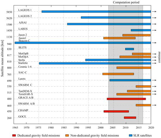
Figure 1.
Mission lifetimes for the satellites at different altitudes ranging from 260 km to 5850 km, including HLSST dedicated gravity satellites (red bars), HLSST non-dedicated gravity satellites (orange bars), and SLR geodetic satellites (blue bars). The grey area is the computation period from January 2003 to August 2016.
The determination of the combined monthly solutions HLSST+SLR was based on the previous work of Weigelt et al. [18] and Sośnica et al. [15]. Weigelt et al. [18] studied the time-variable gravity field from HLSST to CHAMP satellite, whereas Sośnica et al. [15] recovered the monthly models from SLR to multiple geodetic satellites. The principles of the gravity field recovery are both based on the theory of satellite orbit perturbations [28], but they differ in observation type and gravity field recovery approach. In simple terms, for HLSST, precise kinematic LEOs orbits are first determined based on GPS tracking measurements, then total accelerations acting on the satellite are obtained through numerical second derivative of the kinematic satellite positions, namely acceleration method; finally, the Earth gravitational accelerations, i.e., the gradients of the Earth’s gravitational potential, are extracted by separating other measured or modeled forces acting on the satellites. To recover solutions HLSST+SLR, LEOs kinematic orbits were employed from the Astronomical Institute of the University of Bern (AIUB), the Institute of Geodesy at Graz University of Technology (ITSG) and IfE at Leibniz University Hannover. Accelerometer data containing non-gravitational forces information were used if available. For SLR, laser range measurements between ground stations and geodetic satellites are directly used to construct the equations of motion and variational equations. By solving these equations, gravity parameters, together with initial orbit states, station coordinates, etc. were estimated simultaneously.
The combination of HLSST and SLR was performed at the normal equation level. Normal equations established from observation equations of single satellites were weighted and stacked to form the combined normal equation system
where is the normal equation matrix, is the estimated parameter vector containing the spherical harmonic coefficients of the Earth gravity field, is the right-hand side vector, and are the relative weights. Here, the relative weights were based on a priori variance factors. The unknowns of harmonics were estimated in the least square adjustment in the monthly batches.
In GRACE data processing, it is common to apply spatial filtering to suppress noise. Likewise, spatial filtering will be needed for HLSST+SLR solutions with even stronger filtering properties due to the higher noise level of the solution. Here, we apply temporal filtering, besides the spatial filtering, to each time series of coefficients, which enables us to be less aggressive in the spatial domain filtering, i.e., we do not need to apply spatial filtering with a larger scale filtering radius, and thus retain spatial resolution. Obviously, this comes at the cost of a reduced temporal resolution. The short-term events such as flooding are mostly occurring at smaller scales, e.g., river basins, which are largely out of reach for HLSST+SLR solutions. Kalman filtering can be employed to achieve improved results, e.g., as shown in Weigelt et al. [18]. The methodology for the Kalman filter procedure is outlined in Chen, et al. [29].
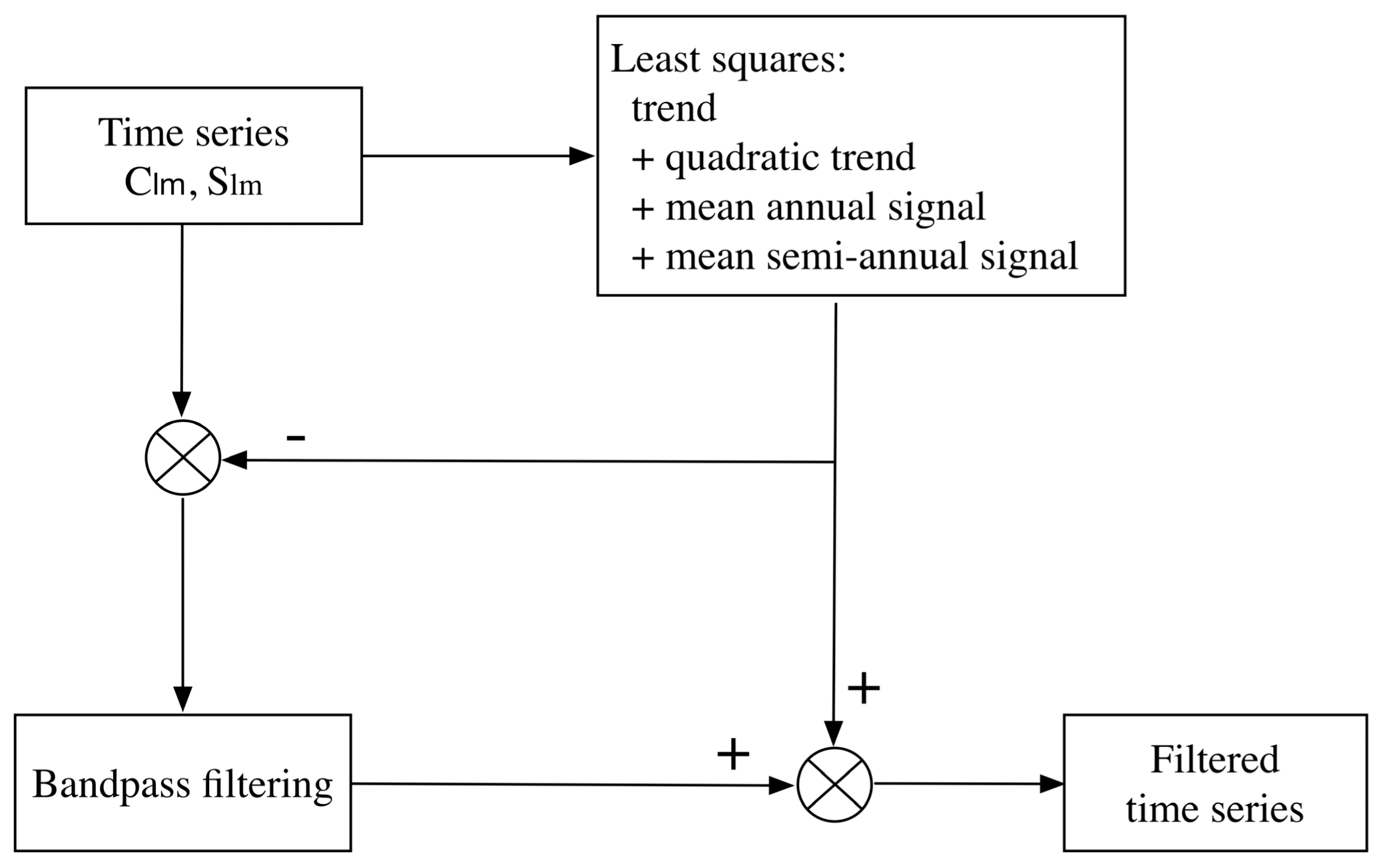
Here, we employ a new way of filtering by using a simple bandpass filter instead of the Kalman filter, thanks to the long time series, i.e., 13 years [30]. The processing flow of filtering is shown in Figure 2. First, the secular trends, quadratic trends, annual and semi-annual signals were extracted and removed from the original time series of a single spherical harmonic potential coefficient in the least square adjustment, similar to Equation (2) in [18]. Subsequently, bandpass filtering is applied to the residual harmonic coefficient time series aiming primarily at retaining the interannual signals and reducing the noise. The practical implementation is done by applying zero-shift filtering with a Butterworth filter twice. In the first run, low frequencies below 0.25 cpy (cycles per year) are filtered by reducing the low-pass filtered time series from the residuals. Subsequently, high-frequency singles are removed by filtering signals with frequencies above 5 cpy. We finally obtained the filtered solutions by adding the bandpass filter output to the extracted mean signals recovered by the least square adjustment.

Figure 2.
Processing flow of filtering. The mean signals, including trend, quadratic trend, mean annual and semi-annual signals, are removed and restored. Bandpass filtering is implemented on the residual harmonic coefficients to reduce noise.
In this paper, to analyze the performance of the HLSST+SLR solutions, other monthly gravity field models were used for the comparison, including GRACE CSR RL06, SLR, and CHAMP solutions. The GRACE CSR RL06 solutions [31] are derived from GRACE LLSST and can be considered as the standard monthly gravity field solutions for most of the spherical harmonics, except for the C20 and C30 coefficients. In the following analysis, these two coefficients were replaced by the SLR-derived values as recommended [9]. The SLR solutions are an extended version of the results from Sośnica et al. [15], with a much longer time series that dates back to 1995. Furthermore, the CHAMP solutions are derived from CHAMP HLSST [18]. We include CHAMP and SLR solutions in the comparison because HLSST+SLR solutions are determined based on CHAMP and SLR solutions; thus, the estimation procedures are similar, making it reasonable to study the improvement of HLSST+SLR solutions over the SLR-only and HLSST-only solutions.
3. Results and Discussion
3.1. Coefficients of the Time-Variable Gravity Ffield
In this section, we evaluate the monthly gravity field solutions HLSST+SLR in terms of spherical harmonic coefficients in the spectral domain. Degree-specific difference amplitudes and degree-specific correlations are two ways to quantify comparisons between two sets of spherical harmonic coefficients. The degree-specific difference amplitudes are calculated using the following equation:
where and denote the differences of spherical harmonic coefficients between two solutions at degree n and order m.
The degree-specific correlations between two sets of coefficients denoted as a set A and a set B are given by
In this study, the degree-specific difference amplitudes of the monthly gravity solutions with respect to the static model EIGEN-6C4 were calculated. It is worth mentioning that when using the degree-specific difference amplitudes, it is necessary to compare gravity fields with the same a priori accuracy. Since the same reference model was used for the comparison, the above limit did not apply. Here, EIGEN-6C4 was set as the reference model because it is inferred from the combination of LAGEOS, GRACE, GOCE, and ground data, and it is more precise and reliable within the spectrum we consider [32]. Figure 3 shows the degree-specific difference amplitudes of the monthly gravity solutions with respect to EIGEN-6C4 over the year 2005. For other periods, the performance characteristics are similar. The black line denotes the degree variances of coefficients of EIGEN-6C4. As expected, GRACE CSR has the highest accuracy over the entire range of the spectrum. Unfiltered HLSST+SLR solutions have the same processing as HLSST+SLR solutions but without applying any filters. The comparison of HLSST+SLR unfiltered solutions and HLSST+SLR solutions demonstrates the significant filtering effect, as in Weigelt et al. [18]. HLSST+SLR solutions show comparable accuracy with GRACE CSR and SLR monthly solutions for spherical harmonic coefficients below degree 10 (about the wavelength of 2000 km). The average ratio of the amplitude of degree variance of HLSST+SLR to GRACE is about 1.5 for harmonics below degree 10, close to that of SLR to GRACE. Above degree 10, the amplitude increases with the degree increases, suggesting that the noise is growing for higher degrees. At degree 20 (about the wavelength of 1000 km), the relative accuracy of HLSST+SLR solutions is 10 times worse relative to that of GRACE CSR. Compared with CHAMP, HLSST+SLR has a visible improvement in the long wavelength of below degree 20, particularly for degree 2 and 6, where the average ratio of amplitude of degree variance of CHAMP to GRACE is greater than 3.0. However, the amplitudes of HLSST+SLR solutions are close to those of CHAMP solutions for degrees above 20. Based on previous studies by Sośnica et al. [15], Cheng and Ries [27], it is believed that SLR contributes to the very long wavelengths (up to degree 10 with the largest impact to degree 5), and multi-HLSST enhances the higher degrees (up to degree 20).
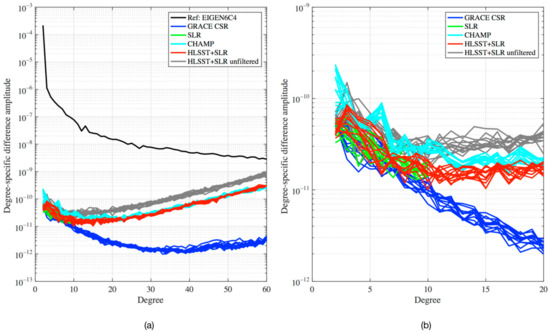
Figure 3.
Degree-specific difference amplitudes of the monthly gravity solutions with respect to EIGEN-6C4 over the year 2005. Figure (a) displays spectrum ranging up to degree 60, while (b) focuses on low degrees ranging up to degree 20. Two sets of solutions—HLSST+SLR solutions and HLSST+SLR unfiltered solutions are shown here. CHAMP is the filtered solutions by applying the Kalman filter. No filtering is applied to GRACE CSR and SLR solutions. The black line is the degree variances of coefficients from EIGEN-6C4.
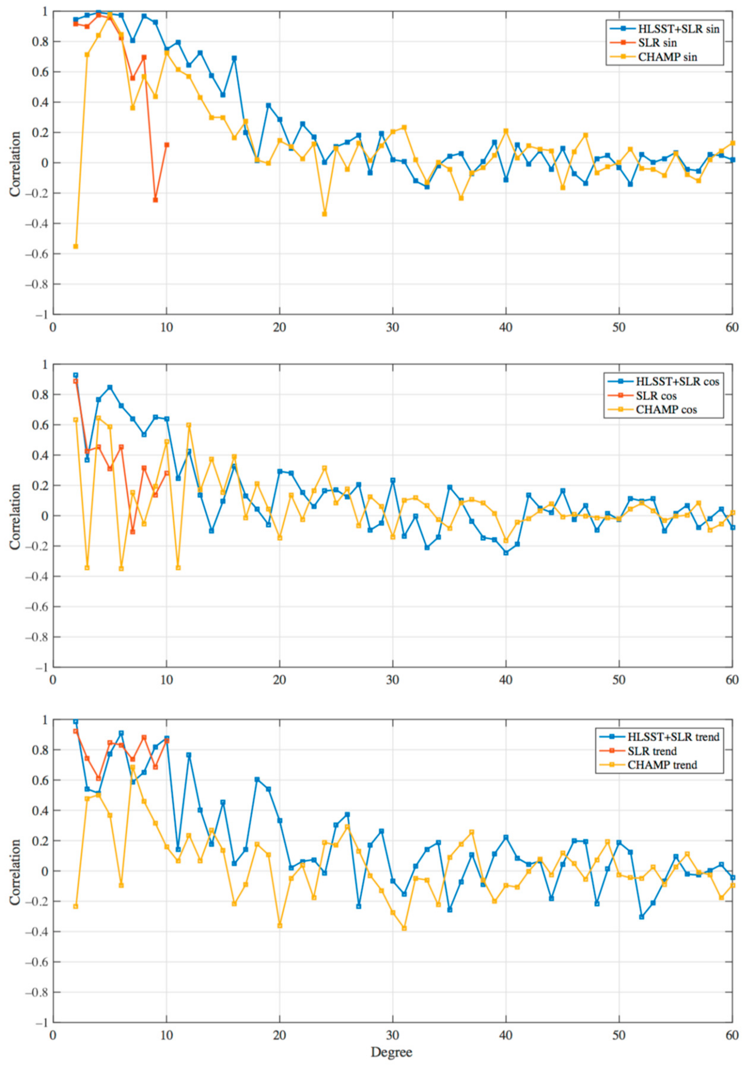
We adopted the concept of degree correlation for the annual cycle between two time-variable spherical harmonic coefficient sets in the supporting material from Tapley, et al. [33], which quantifies the level of correlation of the annual signals of each degree. Indeed, in addition to annual signals, harmonic coefficients contain long-term trends, interannual and other periodic signals, which are also important sources of information for scientific analyses. Thus, the annual signals and long-term trends are considered here. Figure 4 displays the degree correlations for the annual signals and long-term trends of individual HLSST+SLR, SLR, CHAMP monthly solutions with the GRACE CSR solutions during the common period from January 2003 to December 2009. The top, middle, and bottom subgraphs of Figure 4 show the degree correlations of the annual sine term, the annual cosine term, and the long-term trend, respectively. Since the sine components dominate the annual variations, the correlations of the cosine terms (middle plot) are generally smaller than those of the sine terms (top plot), which is in accordance with the supporting material of Tapley et al. [33] and Bezděk et al. [21]. HLSST+SLR and GRACE CSR are highly correlated for harmonics below degree 10, with a correlation greater than 0.8 for the sine terms and mostly greater than 0.6 for the cosine and trend terms. However, the correlation decreases rapidly as the degree increases, with the correlation about 0.2 at degree 20, and becomes completely uncorrelated somewhere about degree 30 (corresponding to spatial features of ~667 km). Except for the trend of SLR, HLSST+SLR solutions have higher correlations with GRACE CSR for harmonics below degree 20 when compared with SLR and CHAMP solutions. Above degree 20, HLSST+SLR and CHAMP solutions cannot describe well the temporal gravity field variations. It is worth noting that the correlation of the SLR annual signals deteriorates above degree 6, but HLSST+SLR still maintains a high correlation level at degree 10, which could be attributed to HLSST GPS data. With SLR dominating the very long wavelengths and HLSST enhancing the spatial resolution, it leads the HLSST+SLR solutions to the comparable level with GRACE CSR solutions for harmonics below degree 10, and in good agreement with the GRACE CSR solutions, but with much noise up to degree 20.
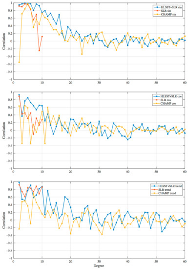
Figure 4.
Degree-specific correlations for the annual sine term (top), the annual cosine term (middle), and the trend (bottom) of HLSST+SLR, SLR, CHAMP monthly solutions with GRACE CSR solutions over the common period from January 2003 to December 2009.
Let us now discuss the spherical harmonic coefficient C20 term. It cannot be well determined by GRACE LLSST, possibly due to system error caused by the thermal effect in the accelerometers onboard the GRACE satellites [27] or S1 and S2 tidal aliasing [34,35]. However, C20 can be accurately obtained from SLR [36,37,38]. Thus, it is recommended that the GRACE C20 estimation should be replaced by the value from SLR in the applications of GRACE-based mass recovery. Since HLSST+SLR solutions use SLR data, we expect that the C20 coefficient of HLSST+SLR solutions could be estimated accurately. While the SLR data used and estimation strategy are different between the HLSST+SLR C20 and the replacement C20, an evaluation of HLSST+SLR C20 is needed. Figure 5 shows a comparison of the time series of the C20 coefficient variations. The time series of HLSST+SLR C20 variation is in good agreement with that used for the replacement, with a correlation of 0.87 and root mean square (RMS) of 5 × 10⁻¹¹. Therefore, HLSST+SLR provides reliable C20 coefficients with no need to replace C20 such as in GRACE solutions.
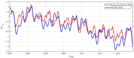
Figure 5.
Spherical harmonic coefficient C20 variation of HLSST+SLR solutions and the replacement value from SLR for GRACE CSR solutions covering period from January 2003 to August 2016.
3.2. Comparison and Analysis of Global Mass Redistribution Recovery
From the analysis in the spectral domain, we have a basic knowledge of HLSST+SLR solutions that they perform comparably with GRACE CSR for degrees below 10, and worse than GRACE CSR for degrees above 10 with much noise, and may be unreliable for degrees above 20. Analysis can also be done in the spatial domain.
The time-variable Earth gravity field provides a novel application for monitoring mass redistribution within the Earth system, both globally and regionally [39]. Therefore, we investigated the capabilities of the HLSST+SLR solutions for measuring global and regional mass transport by comparing them with GRACE CSR solutions. Based on the above analysis, spherical harmonic coefficients of monthly solutions are truncated to degree 10, 15, and 20 to detect the spatial resolution and accuracy level of HLSST+SLR solutions in the application of Earth’s mass change recovery.
In the process of the mass recovery from spherical harmonic coefficients of the gravity field, filtering is usually used to reduce spatial noise, based, e.g., on the Gaussian filter. By applying the filter, the high degree harmonic coefficients, which have great noise, are downweighed; thus, the noise is reduced. In this study, however, to obtain both the original signal content and noise level on the corresponding spatial scale, no filter was used in the mass recovery from all solutions. Additionally, since our goal is not to estimate the true mass change quantities but to make comparisons, some corrections such as post-glacial rebound and leakage error are not made in the recovery process.
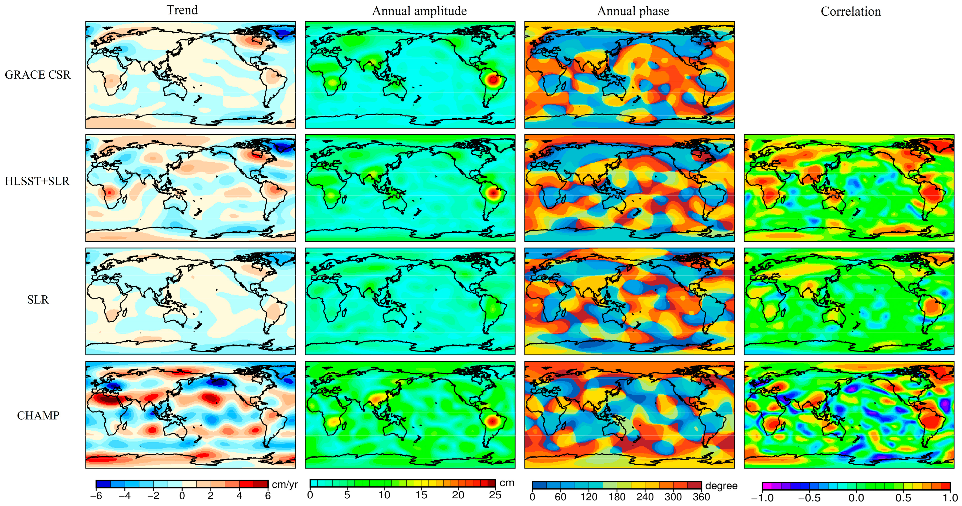
Figure 6 shows the global mass change distribution map derived from monthly time-variable gravity field models (GRACE CSR, HLSST+SLR, SLR, and CHAMP) with spherical harmonic coefficients truncated to degree 10, covering the 11 years of the common period from January 2003 to December 2013. The average trend, annual amplitude, and phase were fitted and displayed from column 1 to column 3 in terms of centimeters of water height equivalent. The fourth column shows the spatial correlation coefficients of mass redistribution with GRACE CSR. Information about the most large-scale mass transport is clearly demonstrated in Figure 6. The trend features in the first column reveal a long-term trend of negative ice sheet mass balance in Greenland. The amplitudes of the annual signals in the second column demonstrate areas with the strongest continental water storage variations, e.g., the Amazon Basin, the Ganges Basin, and the Congo Basin. Figure 6 demonstrates that among the three solutions, the global mass redistribution features from HLSST+SLR agree best with GRACE CSR, not only in the geographical location but also in the magnitude. Correlations between HLSST+SLR and GRACE CSR over Greenland, the Amazon, Ganges, and Congo Basins are greater than 0.8, indicating perfect agreement over these regions. Correlation in the Antarctic is about 0.6, slightly less than for the basins mentioned above. It is mainly due to the difference in annual variations, with an amplitude difference of about 3 cm and a phase difference of about 40 days.
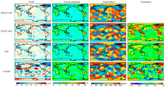
Figure 6.
Trend, annual amplitude, and phase fitted from mass variations derived from GRACE CSR monthly (first row), HLSST+SLR monthly (second row), SLR monthly (third row), and CHAMP monthly (fourth row) solutions in terms of centimeters of water height equivalent. Spatial correlations of mass changes from each kind of solution with the standard GRACE CSR solutions are in the fourth column. The maps are based on monthly solutions covering the 11-year period from January 2003 to December 2013, with coefficients of all solutions truncated to degree 10.
On the whole, about 52% of the global land area is characterized by correlations greater than 0.6 for HLSST+SLR solutions, while only 28% and 16% for CHAMP and SLR, respectively (see Figure 6 and Figure 8). The mean spatial correlation over land reaches 0.58 for HLSST+SLR solutions, while only 0.27 and 0.28 for SLR and CHAMP solutions, respectively. Although in the third and the fourth row CHAMP and SLR solutions show similar features, CHAMP somehow overestimates, whereas SLR underestimates magnitudes of gravity field variations over regions such as the Amazon Basin and Greenland. Moreover, the CHAMP results provide spurious strong trend signals of about +6 cm/y in Northern Africa and −6 cm/y in Southern Europe (row 4, column 1). The mass changes in the ocean are uniformly distributed and weak in magnitude relatively, with the trend of mean sea level rise about 2 mm/y. Thus, it could be an indicator to evaluate the noise level of gravity field solutions. Compared with GRACE CSR, the trend from HLSST+SLR solutions displays noise of 2 cm/y in some ocean regions, while that from CHAMP solutions reveals more noise, up to 5 cm/y, in the middle of the Pacific Ocean.
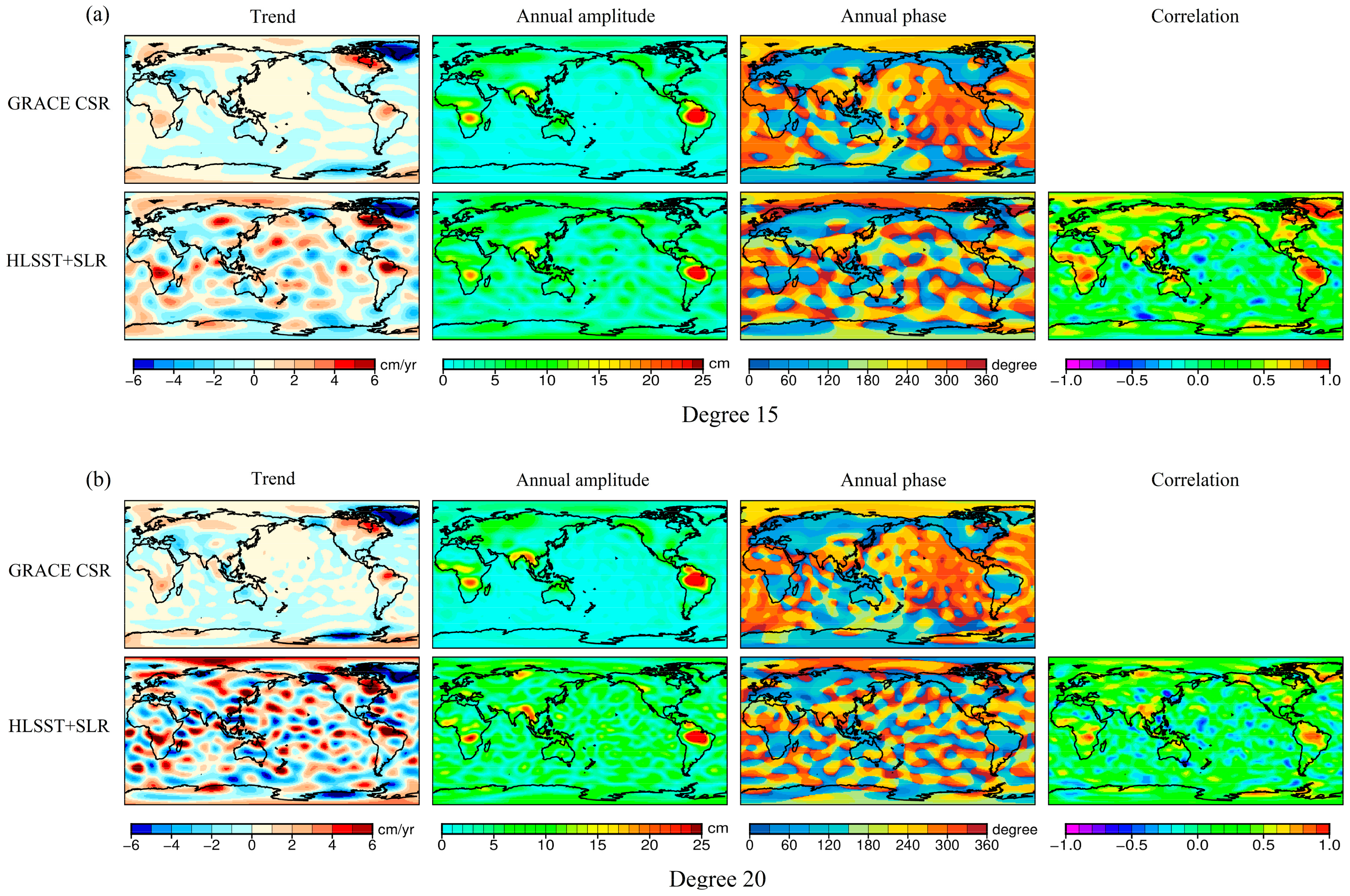
We additionally examine the performance of the mass recovery from HLSST+SLR solutions with spherical harmonic coefficients truncated to degrees 15 and 20. Figure 7a,b show the comparison between GRACE CSR and HLSST+SLR solutions with spherical harmonic coefficients truncated to degree 15 and 20, respectively. For both cases, most of the features have been captured well by HLSST+SLR solutions. Annual variation in the Amazon, Ganges, and Congo Basins and long-term trends in Greenland from HLSST+SLR match well with those from GRACE CSR. The spatial correlations over those regions are larger than 0.8 when truncated to degree 15, and 0.6 when truncated to degree 20. Significant errors lie in the spurious strong trend signals in Siberia and the overestimation of the trend terms in the Amazon and Congo Basins, as we can see in the first column of Figure 7. As the spatial resolution increases, the noise grows. Especially for degree 20, the noise of HLSST+SLR solutions is dominant where the magnitude of mass transport is small. The ocean and some places on land exhibit long-term trends up to 5 cm/y and the annual amplitude up to 10 cm, which are attributed to the noise of spherical harmonics of degree 10 to 20. Over the ocean area 750 km away from the coastline, the RMS of the long-term trend is 2.5 cm/y for HLSST+SLR solutions truncated to degree 20, much larger than 0.4 cm/y for the GRACE CSR solutions truncated to degree 20. Similarly, in terms of amplitude over oceans, the RMS is 5.9 cm, higher than 1.5 cm for GRACE CSR. As a result, the mean spatial correlation over land decreases to 0.35 for truncation to degree 15, and drops to 0.28 for truncation to degree 20.
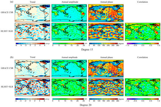
Figure 7.
Trend, annual amplitude, and phase of mass variations derived from GRACE CSR monthly and HLSST+SLR monthly solutions in terms of centimeters of water height equivalent. Spatial correlations of mass change from HLSST+SLR with standard GRACE CSR are in the fourth column. (a) Coefficients of both solutions are truncated to degree 15. (b) Coefficients of both solutions are truncated to degree 20.
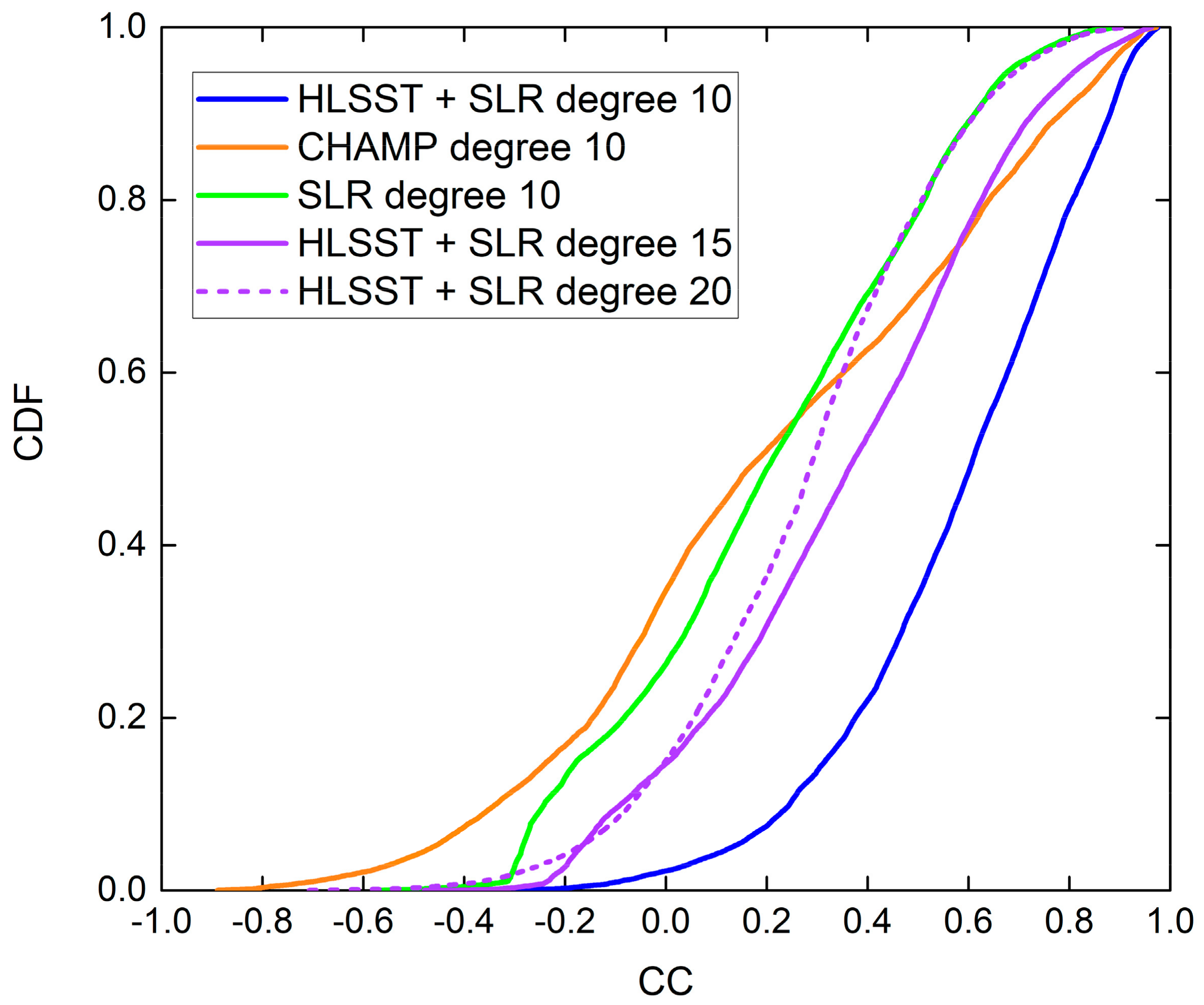
Figure 8 compares the cumulative distribution function (CDF) of spatial correlations from all solutions analyzed above. The spatial correlations only cover the land, since the small mass variation signals over the oceans from HLSST+SLR are usually annihilated by noise. HLSST+SLR solutions with coefficients truncated to degree 10 correlate with GRACE CSR quite well. The slope of cumulative spatial correlation of HLSST+SLR solutions with coefficients truncated to degree 20 begins to steepen at a correlation of 0.2 and becomes horizontal at a correlation of 0.8, illustrating the increase in noise. Despite much noise, HLSST+SLR outperforms the CHAMP and SLR solutions with coefficients truncated to degree 10 with less negative and weak correlations.
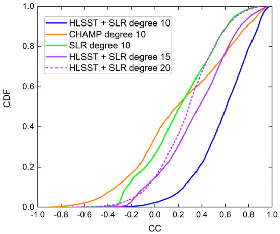
Figure 8.
CDF of spatial correlations derived from HLSST+SLR, CHAMP, SLR solutions with GRACE CSR. CC stands for coefficient correlation.
3.3. Regional Mass Transport Recovery
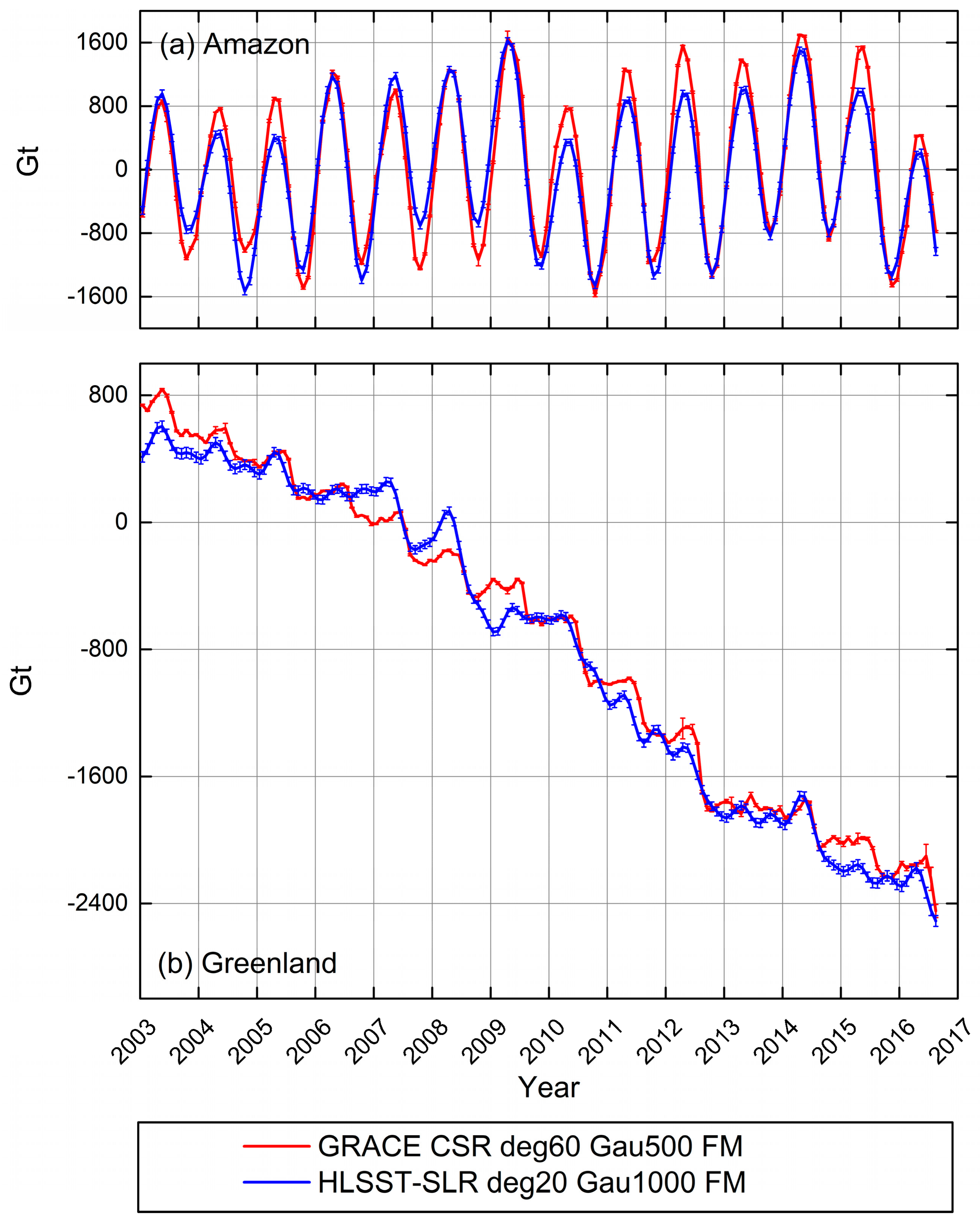
To investigate the capability of recovering large-scale mass redistribution, we selected two typical regions with strong seasonal variations and trends for regional mass transport recovery: the Amazon Basin and Greenland. The Amazon Basin exhibits strong seasonal mass changes, whereas Greenland has a pronounced trend and seasonal signals of ice mass change. The time series of water storage variations over the Amazon Basin and ice mass changes over Greenland derived from the monthly solutions are shown in Figure 9a,b, respectively. The period covers January 2003 to August 2016. Aiming to evaluate the accuracy of regional mass changes from HLSST+SLR solutions, the HLSST+SLR solutions truncated to degree 20 were compared with the GRACE CSR solutions with nominal degree 60, and the latter was used as the reference. The time series of regional mass variations were calculated by multiplying the mass distribution field for a regional mask. In the process of mass recovery, filtering was applied, and some corrections were made. Based on the noise level shown in Figure 7b, the Gaussian filtering [39] with a radius of 500 km and 1000 km were applied to GRACE CSR and HLSST+SLR spherical harmonics, respectively, to reduce the noise. A forward modeling method proposed by Chen, et al. [40] was used to reduce signal leakage and restore the signal strength. A widely used GIA model by A, et al. [41] was adopted to correct the GIA effect. The fitting trend and annual amplitude signals of mass variation time series in those two regions are listed in Table 2, as well as the RMS of the difference between HLSST+SLR and GRACE CSR and the correlation with GRACE CSR.
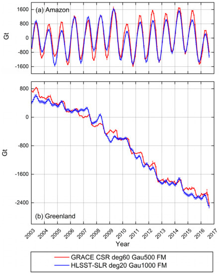
Figure 9.
Time series of mass variations over the Amazon Basin (a) and Greenland (b) derived from GRACE CSR and HLSST+SLR solutions, with coefficients truncated to degree 20 and GRACE CSR nominal degree 60, respectively. Gaussian filtering with a radius of 500 km and 1000 km were applied to GRACE CSR and HLSST+SLR, respectively. The forward modeling (FM) method was used to reduce signal leakage and restore signal strength. The mass variations are values in gigatons. Monthly uncertainties of the recovered mass variations are also shown in the figure. The period covers January 2003 to August 2016.
Table 2.
Trend and annual amplitude of mass flux over the Amazon and Greenland from HLSST+SLR and GRACE CSR solutions, with coefficients truncated to degree 20 and GRACE CSR nominal degree 60, respectively. Gaussian filtering with a radius of 500 km and 1000 km were applied to GRACE CSR and HLSST+SLR, respectively. The RMS of the difference between HLSST+SLR and GRACE CSR and the correlations with GRACE CSR were also calculated.
Over the Amazon Basin, the seasonal variations derived from HLSST+SLR and GRACE CSR are similar, showing distinct annual and interannual variations. The annual amplitude of water storage change over the Amazon Basin from January 2003 to August 2016 is 1019 ± 24 Gt (17 ± 1 cm of water height equivalent) for HLSST+SLR, 143 Gt (2 cm) less than 1162 ± 36 Gt (19 ± 1 cm) for GRACE CSR. Although the interannual variations are displayed clearly, such as the floods in 2009 and the extreme drought in 2005 and 2010, there exist differences in the values of extreme points. The differences mainly occurred in the minimum values in the years 2003, 2007, and 2008, and the maximum values in the years 2004, 2005, and after 2010. Extreme values from HLSST+SLR are underestimated by about 30% than from the GRACE CSR solutions. On the whole, the time series of mass variation over the Amazon Basin shows the RMS of difference between the two solutions of 282 Gt (4.6 cm) and the correlation with GRACE CSR of 0.95.
In Greenland, the trend and seasonal signals are clearly displayed, but some differences are visible. The mass loss trends in Greenland over the period January 2003 to August 2016 agree well, with −245 ± 24 Gt/y for HLSST+SLR and −243 ± 23 Gt/y for GRACE CSR. There is a difference of 29 Gt in the annual amplitude of ice mass variation over Greenland. For HLSST+SLR, the annual amplitude equals 58 ± 19 Gt, whereas for GRACE CSR, the annual amplitude is 87 ± 13 Gt. In general, the time series from HLSST+SLR solutions agrees well with GRACE CSR, with the RMS of the difference between them of 129 Gt and the correlation of 0.99. For HLSST+SLR solutions even truncated to degree 20, the long-term trends of ice sheet mass balance are well captured, while the seasonal signals differ, resulting in a relatively large RMS of difference with GRACE CSR.
4. Conclusions
The HLSST+SLR monthly Earth gravity field solutions are the combination of HLSST to multiple LEOs and SLR to multiple geodetic satellites at the normal equation level. HLSST+SLR employs bandpass filtering with the extraction and restoration of the secular and quadratic trends, annual and semi-annual signals. We analyzed the characteristics of the coefficients of the HLSST+SLR solutions and investigated their capability to recover global and regional Earth’s mass redistributions to determine the spatial resolution and accuracy of the HLSST+SLR solutions.
Analyses in both spectral and spatial domains illustrate that the accuracy of HLSST+SLR solutions below spherical harmonic degree 10 is comparable to that of GRACE CSR and has a pronounced improvement over that of SLR-only and HLSST-only (i.e., CHAMP) solutions. Moreover, the time series of coefficient C20 term of HLSST+SLR solutions agrees well with C20 from SLR due to the contribution of the SLR data. Thus, there is no need to replace the C20 term, such as in the GRACE solutions. Therefore, the consistency of the whole band is ensured. When it comes to the coefficients higher than degree 10 which characterize a higher spatial resolution, the degree-specific difference amplitudes and degree-specific correlations of HLSST+SLR solutions deteriorate, and more noise appears on the mass transport diagram of the HLSST+SLR solutions. Up to degree 20, the HLSST+SLR solutions agree with the GRACE solutions, and the advantage of HLSST+SLR over CHAMP remains. For global mass distribution recovery, most annual amplitudes and some trends can be well derived from HLSST+SLR at the spatial resolution of 1000 km, although the noise over areas of weak mass transport are dominant. In the case of regional mass variation recovery, the seasonal signal of the Amazon Basin and the long-term trend of Greenland derived from HLSST+SLR are perfectly constructed from HLSST+SLR solutions with the spherical harmonic coefficients truncated to degree 20 when compared with the results from GRACE CSR without truncation. The RMS of the time series of mass variations over the Amazon Basin and Greenland is 282 Gt (4.6 cm of water height equivalent) and 129 Gt, respectively.
We confirmed that the combined HLSST+SLR solutions benefit from the individual strengths of HLSST and SLR solutions, enhancing the accuracy of very low degrees, i.e., below degree 10, and improving the spatial resolution to 1000 km. The monthly HLSST+SLR solutions could be another available alternative to study the time-variable Earth gravity field and can be used to monitor the large-scale mass transport such as the water storage of the Amazon Basin and ice mass loss in Greenland during the data gaps between the GRACE and GRACE follow-on missions.
HLSST and SLR, widely applied before the advent of the GRACE missions, can still be seriously taken into consideration today thanks to the best PODs of satellites and the best dynamic models currently available for orbit. Additional LEOs will be equipped with GPS receivers in the future, providing a large number of global continuous and evenly distributed HLSST observation data. The combination of satellites, distributed over different orbital altitudes and inclinations and sensitive to Earth’s gravitational field coefficients of different degrees and orders, may help to obtain a more comprehensive picture of the time-variable Earth gravity field. Furthermore, with the optimization of data processing strategies and further reduction in errors, the combination of HLSST and SLR still has the potential to obtain a time-varying Earth gravity field with higher precision and spatial resolution.
Author Contributions
Conceptualization, K.S. and M.W.; methodology, L.Z.; software, K.S., M.W. and B.L.; validation, K.S., M.W. and B.L.; formal analysis, L.Z. and B.L.; investigation, L.Z.; resources, K.S. and M.W.; data curation, K.S., and M.W.; writing—original draft preparation, L.Z.; writing—review and editing, K.S. and X.Z.; visualization, L.Z. and B.L.; supervision, K.S. All authors have read and agreed to the published version of the manuscript.
Funding
This research was funded by the National Natural Science Foundation of China, grant number 41874021, Ph.D. Short-time Mobility Program of Wuhan University, Basic Research Foundation of the Key Laboratory of Geospace Environment and Geodesy of Ministry of Education, Wuhan University, grant number 41874021 and 19-01-10. M. Weigelt is funded by the Deutsche Forschungsgemeinschaft (DFG, German Research Foundation) under Germany’s Excellence Strategy—EXC-2123 QuantumFrontiers—390837967.
Data Availability Statement
Not applicable.
Acknowledgments
GRACE CSR gravity model solutions and the replacements of C20 and C30 from SLR are available on the Information System and Data Center (ISDC) (ftp://isdcftp.gfz-potsdam.de/grace/ (accessed on 3 June 2021)). Some figures in this paper are generated by using the Generic Mapping Tool (GMT). The authors are grateful to the editor and two reviewers for their helpful comments, which led to a significant improvement for this paper.
Conflicts of Interest
The authors declare no conflict of interest. The funders had no role in the design of the study; in the collection, analyses, or interpretation of data; in the writing of the manuscript, or in the decision to publish the results.
References
- Cazenave, A.; Chen, J.L. Time-variable gravity from space and present-day mass redistribution in the Earth system. Earth Planet. Sci. Lett. 2010, 298, 263–274. [Google Scholar] [CrossRef]
- Tapley, B.D.; Bettadpur, S.; Watkins, M.; Reigber, C. The gravity recovery and climate experiment: Mission overview and early results. Geophys. Res. Lett. 2004, 31, 4. [Google Scholar] [CrossRef] [Green Version]
- Tapley, B.D.; Watkins, M.M.; Flechtner, F.; Reigber, C.; Bettadpur, S.; Rodell, M.; Sasgen, I.; Famiglietti, J.S.; Landerer, F.W.; Chambers, D.P.; et al. Contributions of GRACE to understanding climate change. Nat. Clim. Chang. 2019, 9, 358–369. [Google Scholar] [CrossRef]
- Kornfeld, R.P.; Arnold, B.W.; Gross, M.A.; Dahya, N.T.; Klipstein, W.M.; Gath, P.F.; Bettadpur, S. GRACE-FO: The Gravity Recovery and Climate Experiment Follow-On Mission. J. Spacecr. Rocket. 2019, 56, 931–951. [Google Scholar] [CrossRef]
- Vishwakarma, B.D.; Devaraju, B.; Sneeuw, N. What Is the Spatial Resolution of grace Satellite Products for Hydrology? Remote Sens. 2018, 10, 852. [Google Scholar] [CrossRef] [Green Version]
- Information System and Data Center (ISDC). GRACE Data and Documents. Available online: Ftp://isdcftp.gfz-potsdam.de/grace/ (accessed on 3 June 2021).
- Physical Oceanography Distributed Active Archive Center (PO.DAAC). GRACE Data and Documents. Available online: https://podaac-tools.jpl.nasa.gov/drive/files/allData/grace/ (accessed on 3 June 2021).
- Rietbroek, R.; Fritsche, M.; Dahle, C.; Brunnabend, S.E.; Behnisch, M.; Kusche, J.; Flechtner, F.; Schroter, J.; Dietrich, R. Can GPS-Derived Surface Loading Bridge a GRACE Mission Gap? Surv. Geophys 2014, 35, 1267–1283. [Google Scholar] [CrossRef] [Green Version]
- Loomis, B.D.; Rachlin, K.E.; Wiese, D.N.; Landerer, F.W.; Luthcke, S.B. Replacing GRACE/GRACE-FO C30 With Satellite Laser Ranging: Impacts on Antarctic Ice Sheet Mass Change. Geophys. Res. Lett. 2020, 47, e2019GL085488. [Google Scholar] [CrossRef]
- Nerem, R.S.; Chao, B.F.; Au, A.Y.; Chan, J.C.; Klosko, S.M.; Pavlis, N.K.; Williamson, R.G. Temporal Variations of the Earths Gravitational-Field from Satellite Laser Ranging to Lageos. Geophys. Res. Lett. 1993, 20, 595–598. [Google Scholar] [CrossRef] [Green Version]
- Nerem, R.S.; Eanes, R.J.; Thompson, P.F.; Chen, J.L. Observations of annual variations of the Earth’s gravitational field using satellite laser ranging and geophysical models. Geophys. Res. Lett. 2000, 27, 1783–1786. [Google Scholar] [CrossRef]
- Bianco, G.; Devoti, R.; Fermi, M.; Luceri, V.; Rutigliano, P.; Sciarretta, C. Estimation of low degree geopotential coefficients using SLR data. Planet. Space Sci. 1998, 46, 1633–1638. [Google Scholar] [CrossRef]
- Cheng, M.K.; Tapley, B.D. Seasonal variations in low degree zonal harmonics of the Earth’s gravity field from satellite laser ranging observations. J. Geophys Res. Sol. Ea 1999, 104, 2667–2681. [Google Scholar] [CrossRef]
- Matsuo, K.; Chao, B.F.; Otsubo, T.; Heki, K. Accelerated ice mass depletion revealed by low-degree gravity field from satellite laser ranging: Greenland, 1991–2011. Geophys. Res. Lett. 2013, 40, 4662–4667. [Google Scholar] [CrossRef] [Green Version]
- Sośnica, K.; Jäggi, A.; Meyer, U.; Thaller, D.; Beutler, G.; Arnold, D.; Dach, R. Time variable Earth’s gravity field from SLR satellites. J. Geod. 2015, 89, 945–960. [Google Scholar] [CrossRef] [Green Version]
- Cheng, M.K. Satellite Laser Ranging in 5 × 5 Spherical Harmonics. Available online: https://zenodo.org/record/831745 (accessed on 23 April 2021).
- Reigber, C.; Luhr, H.; Schwintzer, P. CHAMP mission status. Adv. Space Res. 2002, 30, 129–134. [Google Scholar] [CrossRef]
- Weigelt, M.; van Dam, T.; Jaggi, A.; Prange, L.; Tourian, M.J.; Keller, W.; Sneeuw, N. Time-variable gravity signal in Greenland revealed by high-low satellite-to-satellite tracking. J. Geophys Res. Sol. Ea 2013, 118, 3848–3859. [Google Scholar] [CrossRef] [Green Version]
- Bezděk, A.; Sebera, J.; Klokočník, J.; Kostelecky, J. Gravity field models from kinematic orbits of CHAMP, GRACE and GOCE satellites. Adv. Space Res. 2014, 53, 412–429. [Google Scholar] [CrossRef]
- Visser, P.N.A.M.; van der Wal, W.; Schrama, E.J.O.; van den IJssel, J.; Bouman, J. Assessment of observing time-variable gravity from GOCE GPS and accelerometer observations. J. Geod. 2014, 88, 1029–1046. [Google Scholar] [CrossRef]
- Bezděk, A.; Sebera, J.; da Encarnacão, J.T.; Klokočník, J. Time-variable gravity fields derived from GPS tracking of Swarm. Geophys. J. Int. 2016, 205, 1665–1669. [Google Scholar] [CrossRef] [Green Version]
- Jäggi, A.; Dahle, C.; Arnold, D.; Bock, H.; Meyer, U.; Beutler, G.; van den IJssel, J. Swarm kinematic orbits and gravity fields from 18 months of GPS data. Adv. Space Res. 2016, 57, 218–233. [Google Scholar] [CrossRef]
- da Encarnacão, J.T.; Arnold, D.; Bezděk, A.; Dahle, C.; Doornbos, E.; van den IJssel, J.; Jaggi, A.; Mayer-Gurr, T.; Sebera, J.; Visser, P.; et al. Gravity field models derived from Swarm GPS data. Earth Planets Space 2016, 68. [Google Scholar] [CrossRef] [Green Version]
- Gunter, B.C.; Encarnacão, J.; Ditmar, P.; Klees, R. Using Satellite Constellations for Improved Determination of Earth’s Time-Variable Gravity. J. Spacecr. Rocket. 2011, 48, 368–377. [Google Scholar] [CrossRef]
- Weigelt, M.; Jäggi, A.; Meyer, U.; Arnold, D.; Grahsl, A.; Sośnica, K.; Dahle, C.; Flechtner, F. HlSST and SLR-bridging the gap between GRACE and GRACE Follow-on. In Proceedings of the 20th EGU General Assembly Conference Abstracts, Vienna, Austria, 8–13 April 2018; p. 14258. [Google Scholar]
- Pearlman, M.; Arnold, D.; Davis, M.; Barlier, F.; Biancale, R.; Vasiliev, V.; Ciufolini, I.; Paolozzi, A.; Pavlis, E.C.; Sosnica, K.; et al. Laser geodetic satellites: A high-accuracy scientific tool. J. Geod. 2019, 93, 2181–2194. [Google Scholar] [CrossRef]
- Cheng, M.K.; Ries, J. The unexpected signal in GRACE estimates of C20. J. Geod. 2017, 91, 897–914. [Google Scholar] [CrossRef]
- Kaula, W.M. Theory of Satellite Geodesy: Applications of Satellites to Geodesy; Dover Publishing Company: New York, NY, USA, 1966. [Google Scholar]
- Chen, Q.; van Dam, T.; Sneeuw, N.; Collilieux, X.; Weigelt, M.; Rebischung, P. Singular spectrum analysis for modeling seasonal signals from GPS time series. J. Geodyn. 2013, 72, 25–35. [Google Scholar] [CrossRef]
- Weigelt, M.; van Dam, T.; Baur, O.; Tourian, M.; Steffen, H.; Sośnica, K.; Jäggi, A.; Zehentner, N.; Mayer-Gürr, T.; Sneeuw, N. How well can the combination of hlSST and SLR replace GRACE? A discussion from the point of view of applications. In Proceedings of the GRACE Science Team Meeting, Potsdam, Germany, 29 September–2 October 2014. [Google Scholar]
- Bettadpur, S. UTCSR Level-2 Processing Standards Document (For. Level-2 Product Release 0006) (Rev. 5.0, April 18, 2018); Technical Report GRACE. 2018. Available online: ftp://isdcftp.gfz-potsdam.de/grace/DOCUMENTS/Level-2/ (accessed on 2 September 2021).
- Förste, C.; Bruinsma, S.L.; Abrikosov, O.; Lemoine, J.M.; Marty, J.C.; Flechtner, F.; Balmino, G.; Barthelmes, F.; Biancale, R. EIGEN-6C4: The latest combined global gravity field model including GOCE data up to degree and order 2190 of GFZ Potsdam and GRGS Toulouse. GFZ Data Serv. 2014, 10. [Google Scholar] [CrossRef]
- Tapley, B.D.; Bettadpur, S.; Ries, J.C.; Thompson, P.F.; Watkins, M.M. GRACE measurements of mass variability in the Earth system. Science 2004, 305, 503–505. [Google Scholar] [CrossRef] [Green Version]
- Seo, K.W.; Wilson, C.R.; Chen, J.L.; Waliser, D.E. GRACE’s spatial aliasing error. Geophys. J. Int. 2008, 172, 41–48. [Google Scholar] [CrossRef] [Green Version]
- Chen, J.L.; Wilson, C.R.; Seo, K.W. S-2 tide aliasing in GRACE time-variable gravity solutions. J. Geod. 2009, 83, 679–687. [Google Scholar] [CrossRef]
- Cheng, M.K.; Tapley, B.D. Variations in the Earth’s oblateness during the past 28 years. J. Geophys Res. Sol. Ea 2004, 109. [Google Scholar] [CrossRef]
- Cheng, M.K.; Tapley, B.D.; Ries, J.C. Deceleration in the Earth’s oblateness. J. Geophys Res. Sol. Ea 2013, 118, 740–747. [Google Scholar] [CrossRef]
- Bloßfeld, M.; Müller, H.; Gerstl, M.; Štefka, V.; Bouman, J.; Göttl, F.; Horwath, M. Second-degree Stokes coefficients from multi-satellite SLR. J. Geod. 2015, 89, 857–871. [Google Scholar] [CrossRef]
- Wahr, J.; Molenaar, M.; Bryan, F. Time variability of the Earth’s gravity field: Hydrological and oceanic effects and their possible detection using GRACE. J. Geophys Res. Sol. Ea 1998, 103, 30205–30229. [Google Scholar] [CrossRef]
- Chen, J.L.; Wilson, C.R.; Tapley, B.D. Contribution of ice sheet and mountain glacier melt to recent sea level rise. Nat. Geosci. 2013, 6, 549–552. [Google Scholar] [CrossRef]
- Wahr, J.; Zhong, S.J. Computations of the viscoelastic response of a 3-D compressible Earth to surface loading: An application to Glacial Isostatic Adjustment in Antarctica and Canada. Geophys. J. Int. 2013, 192, 557–572. [Google Scholar]


Publisher’s Note: MDPI stays neutral with regard to jurisdictional claims in published maps and institutional affiliations. |
© 2021 by the authors. Licensee MDPI, Basel, Switzerland. This article is an open access article distributed under the terms and conditions of the Creative Commons Attribution (CC BY) license (https://creativecommons.org/licenses/by/4.0/).