Article

Study on Collaborative Emission Reduction in Green-House and Pollutant Gas Due to COVID-19 Lockdown in China

1
State Key Laboratory of Information Engineering in Surveying, Mapping and Remote Sensing, Wuhan University, Wuhan 473079, China
2
CAS Key Laboratory of Spectral Imaging Technology, Xi’an 710119, China
3
School of Remote Sensing and Information Engineering, Wuhan University, Wuhan 473079, China
4
School of Electronic Information, Wuhan University, Wuhan 473072, China
*
Author to whom correspondence should be addressed.
Remote Sens. 2021, 13(17), 3492; https://doi.org/10.3390/rs13173492
Submission received: 19 July 2021 / Revised: 28 August 2021 / Accepted: 31 August 2021 / Published: 2 September 2021
(This article belongs to the Special Issue Remote Sensing of Aerosols and Gases in Cities)

Abstract

:
In recent years, as China’s peaking carbon dioxide emissions and air pollution control projects have converged, scholars have begun to focus on the synergistic mechanisms of greenhouse gas and pollution gas reduction. In 2020, the unprecedented coronavirus pandemic, which led to severe nationwide blockade measures, unexpectedly provided a valuable opportunity to study the synergistic reduction in greenhouse gases and polluting gases. This paper uses a combination of NO2, O3, and CO2 column concentration products from different satellites and surface concentrations from ground-based stations to investigate potential correlations between these monitoring indicators in four Chinese representative cities. We found that XCO2 decreased in March to varying degrees in different cities. It was witnessed that the largest decrease in CO2, −1.12 ppm, occurred in Wuhan, i.e., the first epicenter of COVID-19. We also analyzed the effects of NO2 and O3 concentrations on changes in XCO2. First, in 2020, we used a top-down approach to obtain the conclusion that the change amplitude of NO2 concentration in Beijing, Shanghai, Guangzhou, and Wuhan were −24%, −18%, −4%, and −39%, respectively. Furthermore, the O3 concentration increments were 5%, 14%, 12%, and 14%. Second, we used a bottom-up approach to obtain the conclusion that the monthly averaged NO2 concentrations in Beijing, Shanghai, and Wuhan in March had the largest changes, changing to −39%, −40%, and −61%, respectively. The corresponding amounts of changes in monthly averaged O3 concentrations were −14%, −2%, and 9%. However, the largest amount of change in monthly averaged NO2 concentration in Guangzhou was found in December 2020, with a value of −40%. The change in O3 concentration was −12% in December. Finally, we analyzed the relationship of NO2 and O3 concentrations with XCO2. Moreover, the results show that the effect of NO2 concentration on XCO2 is positively correlated from the point of the satellite (R = 0.4912) and the point of the ground monitoring stations (R = 0.3928). Surprisingly, we found a positive (in satellite observations and R = 0.2391) and negative correlation (in ground monitoring stations and R = 0.3333) between XCO2 and the O3 concentrations. During the epidemic period, some scholars based on model analysis found that Wuhan’s carbon emissions decreased by 16.2% on average. Combined with satellite data, we estimate that Wuhan’s XCO2 fell by about 1.12 ppm in February. At last, the government should consider reducing XCO2 and NO2 concentration at the same time to make a synergistic reduction.

Graphical Abstract

1. Introduction

The emergence of the coronavirus disease 2019 (COVID-19) occurred in 30 December 2019 and was declared a global pandemic by the World Health Organization on 11 March 2020 [1]. In response to the COVID-19 outbreak, the China central government had gradually implemented severe nationwide lockdown measures since the end of January 2020. These measures placed the society of China on hold, significantly reducing the emissions of pollutants. In the past decade, China had experienced several social pauses, including routine ones, such as the Lunar New Year and special events, such as the Olympic game and G20. However, 2020 is a special year because, in the first half of the year, most cities in China were blockaded, and industrial, power, and transportation activities were minimized. In the second half of the year, China’s social activities have gradually returned to normal. Hence, the outbreak of COVID-19 pandemic in 2020 provides an opportunity for the analysis of the carbon cycle and compositional relationship between gases (CO2, NO2, and O3).
Owing to the outbreak of COVID-19, greenhouse gas emissions have changed significantly, especially in developing countries. Before the pandemic, the concentration of carbon dioxide (XCO2) increased by 2 ppm per year over the previous decade, and the global XCO2 increased from 278 ppm (prior to the industrialization era) to 410 ppm in 2020 [2]. However, during the pandemic, Le et al. [3] found that the daily global CO2 emissions decreased by −17% by early April 2020 relative to the mean 2019 levels. Zhu et al. [4] found an abrupt 8.8% decrease in global CO2 emissions (−1551 Mt CO2) in the first half of 2020 compared to the same period in 2019. The International Energy Agency (IEA) used monthly projections of fossil fuel energy demand and estimated a −5% decline in global CO2 emissions from January to April 2020, compared to the same period in 2019 [5]. Moreover, the impacts of lockdown in different regions on air quality were observed [6,7,8,9,10]. Dantas et al., considered the consequences of partial lockdown on air quality and obtained the conclusion that PM10 level was reduced to a low level, and NO2 decreased because of the lockdowns [11]. Sahin et al., explored the consequences of weather on COVID-19 pandemic and concluded that wind showed a positive correlation with COVID-19 cases [12]. Ogen et al., studied the outcome of NO2 on COVID-19 mortality and concluded that long-term exposure to NO2 increased fatalities because of COVID-19 [13]. Xie and Zhu explored the effect of temperature on COVID-19 transmission and found a negative relationship between temperature and increased COVID-19 transmission when the temperature was between 16.8 °C and 27.4 °C [4]. Shi et al., examined the outcome of temperature on COVID-19 transmissions and showed that temperature had a positive linear association with COVID-19 cases when the temperature was lower than 3 °C [14]. These studies provided a scientific basis for the study of the relationship between air pollutants and polluting gases and effective ideas for the prevention and control of pollutants and polluting gases.
These studies analyzed changes in trace gases, emissions, and temperature during the epidemic period in 2020 from different perspectives, but the analysis of trace gas concentration changes in 2020 is rare. Few scholars have studied the XCO2 changes [15,16,17,18,19,20,21,22], meanwhile, the government implemented lockdowns caused by the epidemic has provided us with a good opportunity for this analysis. We have accomplished several works in this article as follows. Firstly, we analyzed changes in monthly averaged concentrations of CO2, NO2, and O3 in Beijing, Shanghai, Wuhan, and Guangzhou. For Beijing, Shanghai, Guangzhou, and Wuhan, the results suggested that the amounts of changes in XCO2 were 0.13, −0.99, −0.89, and −1.12 ppm in February, respectively. The concentrations of NO2 and O3 changed by −24% and 5%, −18% and 14%, −4% and 12%, −39% and 14%, respectively, by comparing data in February 2019 with the Sentinel-Satellite-5 data. Furthermore, for Beijing, Shanghai, Guangzhou, and Wuhan, with regard to the ground monitoring network data, the largest amounts of changes in monthly averaged concentrations of NO2 and O3 were −39% and 14%, −40% and −2%, −61% and 9% in February, respectively. However, for Guangzhou, it is in December, and the decrease in NO2 and O3 is −40% and −12%, respectively. Secondly, we have evaluated the relationship between the variation of XCO2 and the variation of NO2 and O3. We found the effect of NO2 concentration on XCO2 is positively correlated from the point of the satellite (R = 0.4912) and the point of the ground monitoring stations (R = 0.3928). Furthermore, we found that XCO2 and O3 are correlated, with a correlation coefficient of 0.2391(from satellite observations) and −0.3333 (from ground monitoring stations). Therefore, from the point of promoting the reduction in XCO2 in atmosphere, the contribution of NO2 concentration is greater than that of O3 concentration. Moreover, the government should consider reducing XCO2 and NO2 concentration at the same time to make a synergistic reduction. The remaining parts of this work are arranged as follows. The data and method we used are described in Section 2. The main results and discussions are demonstrated in Section 3. Finally, we conclude the whole study in Section 4.

2. Materials and Methods

2.1. Study Area

In this paper, four locations were selected: Beijing, Shanghai, Guangzhou, and Wuhan. The main reasons are as follows. First, the Beijing, Shanghai, and Guangzhou are international cities and are located at different latitudes [10], whereas Wuhan is the first epicenter of COVID-19 around the world and is the most important city in central China in terms of economy, education, innovation, and industry; the climatic characteristics of these metropolitan areas are quite different. Therefore, these cities provide good conditions for studying changes in CO2, NO2, and O3 concentrations amid the COVID-19 lockdown in different regions. We show the spatial location distribution of the research area in detail in Figure 1.

2.2. Datasets

2.2.1. Remotely Sensed Products

We analyzed changes in the monthly averaged concentrations of CO2, NO2, and O3 in 2020. For NO2 and O3 data, we used a Sentinel-5 Precursor offline level 3 product [23], which was obtained from the Google Earth Engine platform [24]. The Sentinel-5 Precursor is a satellite launched on 13 October 2017 by the European Space Agency to monitor air pollution. Owing to the incomplete data of O3 and NO2 in 2018, we used data from January 2019 to December 2020.
As for CO2 data, the GOSAT_FTS_L3_V2.95 data of bias-corrected [25] from January 2016 to December 2020 were selected. The Gosat and Gosat-2 satellites have been in orbit since 2009 and 2018, respectively, and their global coverages holds the potential to reveal new information about the carbon cycle by top-down atmospheric inversion methods combined with column-average CO2 retrievals. The GOSAT satellite embarks the Thermal and Near-infrared Sensor for carbon Observation (TANSO) to characterize the column abundances of CO2 and CH4. Six of the seven data channels of this sensor operate in the near-infrared part of the solar spectrum, so this device cannot be used whenever the planet reflects little solar light, i.e., in polar regions during winter. For additional information on that instrument, please consult this website [26]. Besides, a suite of passive remote sensing satellites can measure the reflected sunlight spectra in the infrared region over the globe. These measured spectra are used to retrieve the column-averaged CO2 concentration (XCO2) (e.g., GOSAT, GOSAT-2, OCO-2, OCO-3, and TanSat). However, the interference of clouds and aerosols in XCO2 retrieval often results in sparse spatial and temporal coverage. Therefore, there is no data for these latitudinal regions in China, namely latitudes higher than 48.7°N in December, higher than 51.2°N in November and higher than 51.3°N in January.

2.2.2. Ground Monitoring Data

To further explore the relationship of changes in monthly averaged NO2 and O3 concentrations with XCO2, a bottom-up approach was adopted for analysis, and ground monitoring data were used. The China Air Quality Network includes daily averaged gas concentration changes in China [27]. Hence, along with remotely sensed data, the ground monitoring data were also included in this work. In addition, to evaluate the accuracy of the monthly averaged CO2 concentration data from our algorithm, we used the TCCON (Hefei site) data. The Total Carbon Column Observing Network (TCCON) [28,29] is a network of ground-based Fourier transform spectrometers that record direct solar spectra in the near-infrared spectral region. From these spectra, accurate and precise column-averaged abundances of CO2 are retrieved and reported. For the period of this data and the purpose for which the data are used, we explain in detail in Table 1.

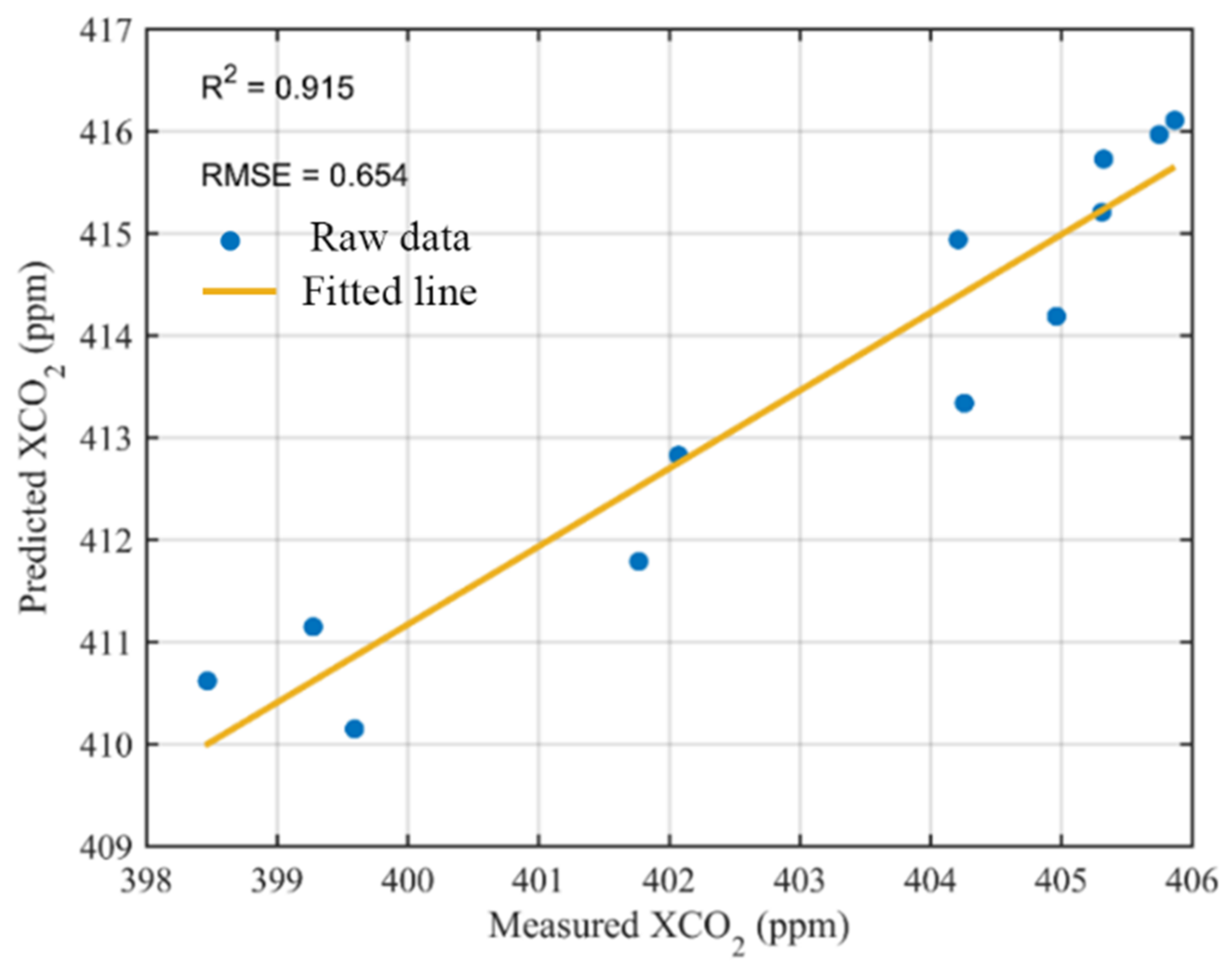
2.3. Analysis Method

This paper mainly adopted a comparative approach for analyzing the impact of the COVID-19 lockdown on the atmospheric environment in 2020. Hence, our work mainly focused on the following four points in detail. Firstly, given the bias-corrected GOSAT_FTS_L3_V2.95 productions are discrete point data, we used the empirical bayesian kriging (EBK) interpolation theory to fill the data gaps in the study area [30]. Additionally, the EBK method is a ground statistical interpolation method that automatically performs the most difficult steps in building an effective kriging model [31,32,33]. The EBK method differs from other kriging methods in illustrating the error introduced by estimating a basic semivariogram. Other kriging methods underestimate the standard error of prediction because they do not consider the uncertainty involved in this semivariogram estimation [33]. For NO2 and O3 planar product data, we directly used it. Second, for GOSAT and GOSAT-2 satellites and ground monitoring data in 2016, 2017, 2018, and 2019, we obtained standard curves using locally weighted regression (LWR). The LWR is a nonparametric method. In each prediction of new samples, the adjacent data will be retrained to obtain new parameter values, to avoid under-fitting and reduce the interference of distant data effectively. Third, we analyzed change in XCO2 by comparing the standard curve data in 2020. To analyze the concentration influence of NO2 and O3 on the change in CO2 concentration, we used the top-down method and bottom-up method, respectively. The investigation of local processes, construction of models, and extrapolation with spatial data to larger scales has been called the “bottom-up” approach. The “top-down” approach aims to obtain data values over a large area in a short period of time without knowing the underlying details of the data caused by subtle scale changes. Therefore, the top-down and bottom-up approaches are thus complementary, and we comprehensively analyzed the influences of NO2 and O3 concentrations on change in XCO2 with satellite data and ground monitoring data in a “multiple constraint” approach.

3. Results and Discussions

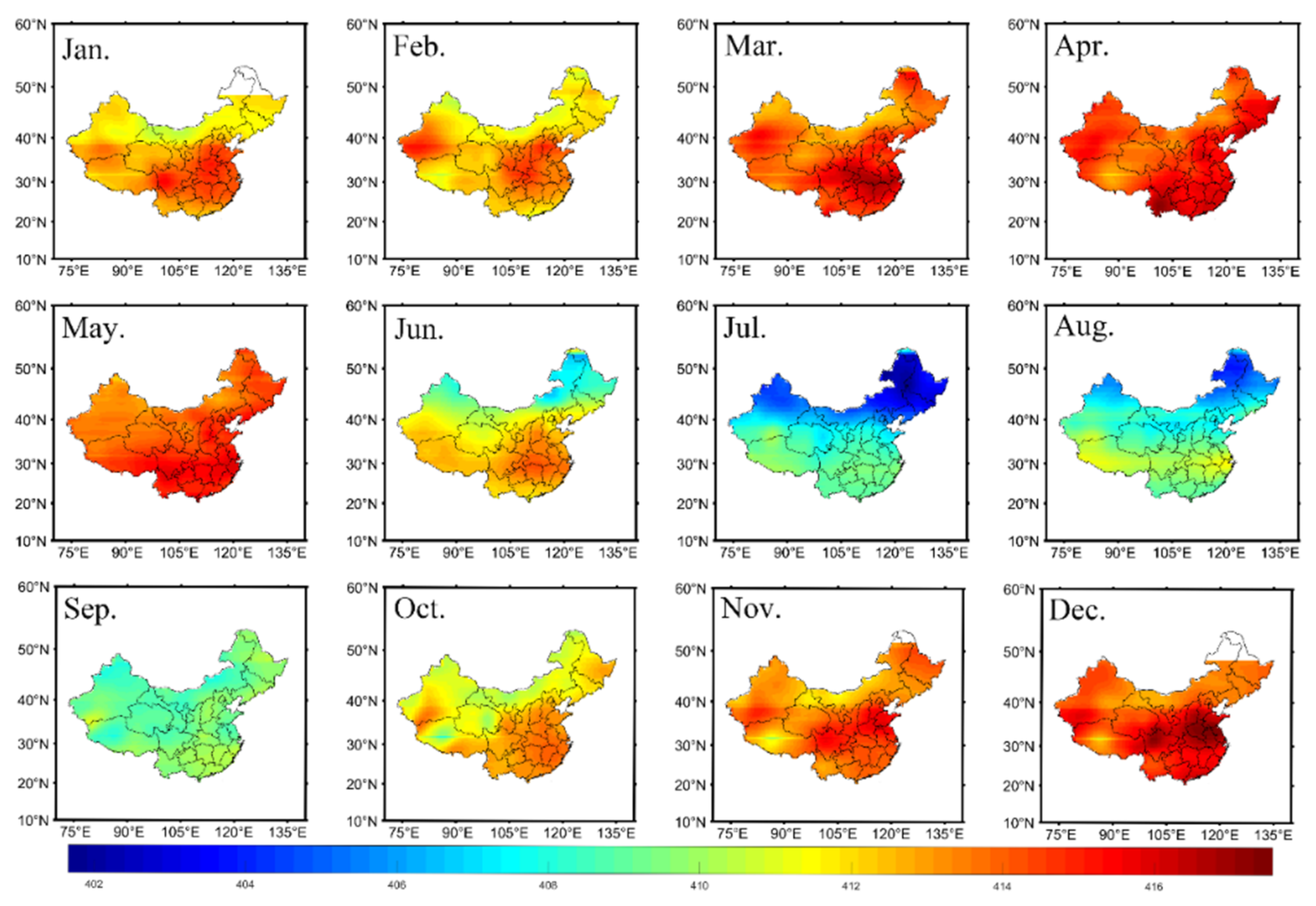
3.1. Spatial Distribution of Remotely Sensed CO2 Concentrations

GOSAT and GOSAT-2 provide passive inversion data and are particularly vulnerable to cloud, aerosol, latitude, and dark night constraints, which cause loss of satellite observation data. We utilized GOSAT_FTS_L3_V2.95 productions, as described in Section 2, and completed the conversion of the GOSAT and GOSAT-2 data points to the surfaces by adopting empirical bayesian kriging (EBK) theory. The data of vacant areas in the study area were filled. Figure 2 shows the interpolated data by using only EBK theory in 2020. Given that the atmospheric environment in China is complex and GOSAT and GOSAT-2 are particularly sensitive to aerosols and clouds, the data gaps in eastern and central China were large. Moreover, the Hainan and Taiwan Provinces as well as the South China Sea are not marked on the local maps in Figure 2. Fortunately, in this case, we were able to use the EBK theory to complete the monthly averaged spatial interpolation on the 0.25° grid.
The Total Carbon Column Observing Network (TCCON) is a network of ground-based Fourier transform spectrometers recording direct solar spectra in the near-infrared spectral region [26]. From these spectra, accurate and precise column-averaged abundances of CO2 are retrieved and reported. In addition, we evaluated the accuracy by combining TCCON site (Hefei [29]) data in 2016 (as shown in Figure 3), and the coefficient of determination (R2) and root-mean-square error (RMSE) were 0.915 and 0.654, respectively.

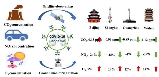
3.2. Analysis of Changes in XCO2

Multiple pixels in the sub-study areas were found because the spatial resolution of the products after interpolation was 0.25°. To evaluate the influence of COVID-19 on the XCO2 of each month in 2020, we matched the five-year XCO2 curve to a scale from 2016 to 2020. First, we set the 2019 XCO2 data as a baseline and then unified the 2016, 2017, 2018, and 2020 XCO2 to the 2019 baseline by revising the annual XCO2 curve increments. This increment was revised using the annual XCO2 curve increments at Waligura stations from global atmosphere watch in China [34]. By performing local weighted regression on all grid XCO2 changes in the current sub-study, the grid scale XCO2 changes were converted to city scale. Because cities vary in development and geographical location, we added a city increment for each city relate to the annual XCO2 curve increments. We use the standard deviation as the city increment, which is the difference between the XCO2 for each month in 2020 and the trend line XCO2. We studied the change in the monthly averaged XCO2 of the city. The image resolution was 0.25 degree after interpolation, and the average amount of change in several pixels contained in each city was obtained.
Then, we tested the revised XCO2 data in 2020 using the Kruskal–Wallis test. The Kruskal–Wallis test is a nonparametric test of three or more datasets. It is used to test the consistency of the null hypothesis and its alternative hypothesis about differences between at least two samples of a population function distribution. A standard is usually used in evaluating significance. The P value is 0.05. If the P value is less than or equal to 0.05, difference between two samples are considered statistically significant; otherwise, they are considered insignificant. A significant difference between the two samples indicated that the XCO2 data in 2020 and local weighted regression XCO2 from 2016 to 2019 were independent. That is, when the P value in Figure 4 is less than 0.05, it indicates that the prevention and control measures during this epidemic period caused this change. For the period from February to May in Wuhan, the P value was less than 0.05. For the period from March to April in Beijing, the P value is also less than 0.05, and for Shanghai and Guangzhou in February, the P value is also less than 0.05. The above results show that the monthly averaged XCO2 in 2020 changed relative to the trend line data; the variation in XCO2 concentration is shown in Figure 5.
Due to the impact of COVID-19 in Beijing, Shanghai, Guangzhou, and Wuhan, Figure 5 shows the monthly averaged XCO2 changes values in 2020. The Chinese government has taken lockdown measures in most Chinese cities from the end of January to early April. Therefore, the XCO2 fluctuates relatively sharply during the period. We found the amounts of changes in XCO2 were 0.13, −0.99, −0.90, and −1.12 ppm in February, for Beijing, Shanghai, Guangzhou, and Wuhan. Then XCO2 continued to decrease from March to May in Beijing. In Shanghai and Guangzhou, both international cities, XCO2 gradually returned to normal levels in April and March, respectively.
Notably, the trend of XCO2 in June, July, and August varied between the coastal cities (Shanghai and Guangzhou) and the inland cities (Beijing and Wuhan). Furthermore, this difference is a combination of effects resulting from seasonal impact weights and the corresponding intensification of industrial emissions. The weight of the seasonal impact of XCO2 gradually increased in June, July, and August. The weight of seasonal influence represents the enhancement of CO2 absorption capacity from surface vegetation. Besides, by analyzing the change in NO2 concentration from June to August in Figure 6, we found that the corresponding industrial emissions of Beijing and Wuhan gradually increased in the three months. Therefore, under the combined action of these two factors, the amounts of changes in XCO2 in June, July, and August in Beijing were 1.54, −0.92, and 0.90 ppm, respectively. In addition, the amounts of changes in XCO2 in Wuhan were 1.30, −0.70, and 1.1 ppm.
For coastal cities of Shanghai and Guangzhou, there are some differences in the change in CO2 concentration. Although Shanghai and Guangzhou are coastal cities, the latitude of Guangzhou is lower than that of Shanghai, and this condition increases the absorption effect of XCO2 brought by season in Guangzhou. In addition, Guangzhou’s geographical proximity to Zhaoqing, an industrial city, increases the dispersion of XCO2 in Guangzhou. In this case, the amounts of changes in XCO2 in June, July, and August were −0.29, −0.57, and 0.49 ppm. However, as the engine of China’s economy, Shanghai’s industrial recovery speed is extremely fast (XCO2 was fully recovered in April, and the XCO2 in May and June showed an upward trend), and industrial emission intensity is increasing. Therefore, under the action of increasing seasonal factors, the XCO2 in June, July, and August showed a gradually increasing trend, with values of 0.41, 0.08, and 1.20 ppm.
In September and October, the amounts of changes in XCO2 remained 0 ppm in the inland cities of Beijing and Wuhan. For the coastal cities of Guangzhou and Shanghai, the amounts of changes in XCO2 remained 0 ppm in September, but the amounts of changes in XCO2 were 0.57 and −0.35 ppm in October, respectively. This phenomenon is related to the prevention and control measures of the local government [35,36,37] and the industrial structure of the surrounding cities. In November and December, the Chinese government strengthened control measures to prevent the recurrence of the epidemic in winter. Second, the annual curve of XCO2 are the interval of the increase in XCO2 in November and December. Therefore, under the action of the above two factors, the amounts of changes in XCO2 were 0 ppm in Beijing and Guangzhou. However, in Wuhan and Shanghai, the amounts of changes in XCO2 fluctuated in November and December. The first outbreak of the epidemic in Wuhan, China lasted for a long time and had a significant effect on reducing the production vitality of some industrial companies in Wuhan [38]. The Shanghai’s XCO2 dropped in December because the Shanghai government had to strengthen the prevention and control of the epidemic after local cases emerged [37,39].
The epidemic affected Wuhan mainly in two periods, from January to May and from November to December. In Guangzhou and Shanghai, the effects were mainly from January to March and in December. Beijing is the political and economic center of China; its XCO2 were affected by the outbreak from March to May, and the significant change occurred in March. In addition, the greater variation of XCO2 was due to the seasonal effects in June, July, and August.

3.3. Analysis of Changes in the Concentration of Gases (NO2 and O3) from Top-Down and Down-Top, Respectively

Given that only 2019 and 2020 had complete data, we directly used Sentinel-5 Premonitory Offline Level 3 products. We obtained the monthly averaged NO2 and O3 data by determining the mean value in each study area. In this section, we compared the data detected in 2019. Figure 6 show the specific monthly averaged concentration (NO2 and O3) and increment changes in 2019 and 2020. The monthly averaged increment represents the increase in concentration from the previous month and to the current month.
Transport and industrial production are the main sources of NOX emissions, and thus the monthly averaged NO2 concentration changes can reflect the cessation of productivity during the epidemic and the recovery of productivity after the epidemic. Figure 6 shows the concentration and increment change in NO2 and O3 in 2019 and 2020, respectively. In Figure 6, the curve of NO2 concentration increment fluctuates mainly from February to May in 2019 and 2020, consistent with the duration of the epidemic released by the Chinese authorities [40]. During the epidemic outbreak, industrial emissions and traffic decreased to a large extent in all parts of China. In the atmosphere, compared with that in February 2019, the amplitude of NO2 concentration in 2020 in Beijing, Shanghai, Guangzhou, and Wuhan decreased by 2.52 × 10⁻⁵, 2.32 × 10⁻⁵, 0.25 × 10⁻⁵, and 3.46 × 10⁻⁵ mol/m2, respectively. The percentage decrease was 24%, 18%, 4%, and 39%, respectively. Then, in March, April, and May, the monthly averaged increase in NO2 concentration in 2020 was smaller than that in 2019. Change in NO2 concentration recovered to the 2019 level from June to December, indicating that the epidemic in China has been brought under control and industrial production has recovered [40]. From February to June 2020, the NO2 concentration decreased, but the O3 concentration showed an increasing trend (Figure 6). Specifically, in February 2020, O3 concentration increments in Beijing, Shanghai, Guangzhou, and Wuhan were 0.851 × 10⁻², 1.55 × 10⁻², 1.24 × 10⁻², and 1.66 × 10⁻² mol/m3, respectively. The decrease percentage was 5%, 14%, 12%, and 14%, respectively. In addition, the increment change in O3 concentration was extended to June, a month longer than the increment change time of NO2 concentration. Similarly, in March, April, May, and June, the monthly averaged increase in O3 concentration in 2020 was smaller than that in 2019. From July to December in 2020, the O3 concentration increment in each region gradually returned to the normal state.
To further analyze the effect of NO2 and O3 concentration on the change in XCO2, we analyzed the daily averaged data of monitoring stations in the ground cities. Given that China’s big events are held according to traditional holidays (Spring Festival and National Day), we matched the 2020 and 2019 time series according to the Lunar New Year. We obtained monthly averaged ground station data by averaging the daily averaged data of monitoring stations in the ground cities. Figure 7 shows the daily averaged and monthly averaged concentration change in NO2 and O3 in 2019 and 2020, respectively. We learned that the daily averaged NO2 concentration in Beijing decreased in 11 February. The daily averaged and monthly averaged concentrations in 2020 were lower than those in 2019 from 11 February to 31 October because the prevention and control measures were strict in Beijing. The monthly averaged distribution of NO2 concentrations began to decline in February, briefly returned to normal in November, and began to decline again in December. The largest annual decline in March was 15.56 µg/m3 in Beijing. The percentage decline was 39%. NO2 concentration decreased, whereas O3 concentration increased by 4.23 µg/m3 in February. The percentage increase was 5%. The monthly averaged NO2 concentration decreased in March and April, and the corresponding monthly averaged O3 concentration in the surface cities showed an obvious trend of decreasing initially and then increasing.
In the monthly averaged NO2 concentration of Shanghai, the trends in change in NO2 concentration in the ground monitoring stations and satellite data were similar. NO2 concentrations at the ground monitoring stations declined from February to May, then the decline rate reached its maximum value in March, with a maximum value of 20.64 µg/m3. The percentage decline was 40%. Subsequently, the NO2 concentrations returned to normal levels but fluctuated from June to November. Finally, in December, NO2 concentrations dropped again in 2020 compared with those in 2019 because the Shanghai government introduced management measures to prevent the recurrence of the epidemic [37,39]. Regarding the monthly averaged O3 concentration, the rising months in 2020 were February, April, September, and November. The daily averaged NO2 concentration decreased from 15 February to 28 February, from 1 April to 22 April, from 1 September to 11 September, and from 1 November to 15 November.
For the monthly averaged NO2 concentration in Guangzhou, the interval of decrease in 2020 can be divided into three parts: from February to March, from July to August, and from October to December. The maximum decrease was found in December, and the maximum value was 27.16 µg/m3. The percentage decline was 40%. The monthly averaged O3 concentration in Guangzhou increased in February and May, and the corresponding daily averaged NO2 concentration decreased from 6 February to 28 February and from 10 May to 21 May. These effects may have been due to the latitude and typhoon because the latitude in Guangzhou is extremely low.
Wuhan is the first Chinese city to have an epidemic case and, thus, has a long shutdown time. We further analyzed the impact of NO2 and O3 on XCO2 in each month in 2020. Two periods of decrease in the monthly averaged NO2 concentration were found at the ground monitoring stations, namely, from February to May and from December to December. The maximum decrease was found in March, with a maximum value of 33.02 µg/m3. The percentage decline was 61%. The monthly averaged O3 concentration in Wuhan increased from February to March and from November to November. The daily averaged NO2 concentration first decreased and then increased from 14 February to 27 March. During this period, the monthly averaged O3 concentration was higher than that in the same period in 2019, and the rate of increase in the monthly averaged O3 concentration in March gradually slowed down compared with that in February. We found that the monthly averaged O3 concentration in Wuhan in November 2020 decreased more slowly than that in 2019 and higher than that in 2019. In addition, during this period, the daily averaged NO2 concentration decreased rapidly from 21 November to 30 November, with a value of 32.90 µg/m3.
Figure 8 shows the percentage and concentration changes for O3 and NO2 for the four study areas from the satellite observation and the ground monitoring stations observation, respectively. In Figure 8a,b, the maximum monthly averaged concentration changes of NO2 and O3 are shown form satellite observation, respectively. In Figure 8c,d, the maximum monthly averaged concentration changes of NO2 and O3 are shown from ground monitoring stations, respectively. Then, we show the different changes for four cities in each subgraph. For each of the subgraphs, the gray and blue bars represent percentage data and concentration change data, respectively. In general, for the satellite observation estimates, the maximum monthly averaged NO2 concentrations in Beijing, Shanghai, Guangzhou, and Wuhan in February 2020 were −24% (−2.52 × 10⁻⁵ mol/m2), −18% (−2.32 × 10⁻⁵ mol/m2), −4% (−0.25 × 10⁻⁵ mol/m2), and −39% (−3.46 × 10⁻⁵ mol/m2), respectively. The corresponding changes in O3 concentration were 5% (0.85 × 10⁻² mg/m3), 14% (1.55 × 10⁻² mg/m3), 12% (1.24 × 10⁻² mg/m3), and 14% (1.66 × 10⁻² mg/m3). In addition, we further evaluated the monthly averaged data from the daily averaged data in the ground monitoring stations. Surprisingly, the assessment showed that February was not the biggest month of variability in NO2 concentrations from ground monitoring stations. The monthly averaged NO2 concentrations in Beijing, Shanghai, and Wuhan in March had the largest changes, changing to −39% (−15.56 µg/m3), −40% (−20.64 µg/m3), and −61% (−33.02 µg/m3). The corresponding amounts of changes in monthly averaged O3 concentrations were −14% (−11.71 µg/m3), −2% (−1.86 µg/m3), and 9% (−7.63 µg/m3). However, the largest amount of change in monthly averaged NO2 concentration in Guangzhou was found in December, with a value of −40% (−27.16 µg/m3). The amount of change in O3 concentration was −12% (−10.46 µg/m3) in December.

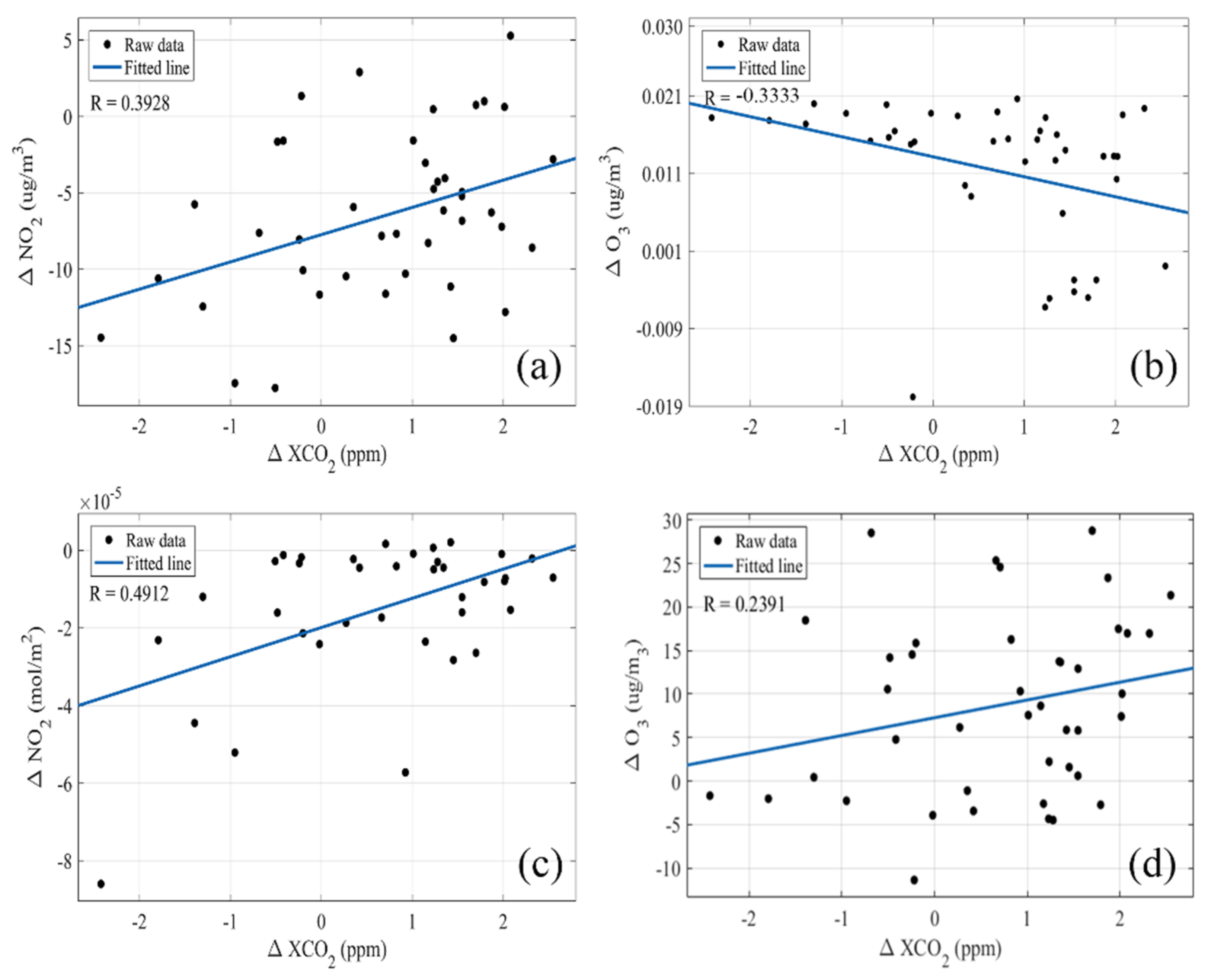
3.4. The Relation of NO2 and O3 Concentration on XCO2

From the perspective of satellite and ground monitoring stations observations, we quantitatively show the effect of NO2 concentration and O3 on XCO2 in Figure 9 from top-down and bottom-up. Figure 9 shows the relationship between the monthly averaged variation of XCO2 observed by satellite and the monthly averaged concentration of NO2 and O3 observed by satellite (Figure 9c,d) and ground monitoring stations observations (Figure 9a,b) in February 2020 relative to 2019, respectively. To avoid the error influence of the interpolation theory of XCO2, and to accurately reflect the interaction relationship of XCO2 on NO2 and O3 concentration, the XCO2 data were adopted from the original point data of GOSAT_FTS_L3_V2.95 in this chapter, and the data processing theory has not changed. Similarly, we obtained monthly averaged differences in the concentrations of NO2, O3, and CO2 in February 2020 relative to 2019. We have evaluated a correlation between the variation of XCO2 and the variation of NO2 and O3 in Figure 9. CO2 and NOx emissions derive from industries and traffic. Therefore, a reduction in emissions corresponds to a reduction in concentrations [38,39]. The variations of XCO2 and NO2 should be correlated (as shown in Figure 9a,c), and their correlation coefficients are 0.4912 (from satellite observation) and 0.3928 (from ground station observation), respectively. On the other hand, tropospheric O3 derives from nonlinear photochemical reactions of the NOx and VOC precursors. Thus, a reduction in NO2 can even cause an increase in O3. For this reason, it is possible that XCO2 and O3 (ground stations) are correlated, with a correlation coefficient of −0.3333.
From the point of promoting the reduction in XCO2 in atmosphere, the contribution of NO2 concentration is greater than that of O3 concentration. However, the relationship between O3 concentration and aerosols was strong because of photochemical reactions [41,42]. Therefore, we can regulate the concentration of O3 by improving the aerosol. In general, from both top-down and bottom-up perspectives, we conclude that we can further improve carbon emissions by regulating NO2 concentrations, but O3 has a relatively small impact on the improvement of XCO2.

4. Conclusions

In this work, we analyzed abnormal XCO2 changes in Beijing, Shanghai, Guangzhou, and Wuhan in each month in 2020, and combined the Sentinel-5 Precursor Offline Level 3 product and the ground monitoring network to analyze the effects of NO2 and O3 concentrations on changes in XCO2 with top-down and bottom-up methods, respectively. We found significant differences in the monthly averaged concentrations of CO2, NO2, and O3. For Beijing, Shanghai, Guangzhou, and Wuhan, the results suggested that the amounts of changes in XCO2 were 0.13, −0.99, −0.89, and −1.12 ppm in February. Furthermore, the concentrations of NO2 and O3 changed by −24% and 5%, −18% and 14%, −4% and 12%, −39% and 14% by comparing data in February 2019 with the Sentinel-Satellite-5 data. Moreover, for Beijing, Shanghai, Guangzhou, and Wuhan, with regard to the ground monitoring network data, the largest amounts of changes in monthly averaged concentration of NO2 and O3 were −39% and 14%, −40% and −2%, and −61% and 9% in February. However, the largest monthly averaged NO2 concentration change in Guangzhou occurred in December, with a value of −40%. Thus, the O3 concentration change was −12% in December.
In addition, we evaluated the relationship between the variation of XCO2 and the variation of NO2 and O3 in Figure 9. CO2 and NOx emissions derive from industries and traffic. Therefore, a reduction in emissions corresponds to a reduction in concentration [40]. The variations of XCO2 and NO2 should be correlated [43]. Additionally, the results also show that the effect of NO2 concentration on XCO2 is positively correlated from the point of the satellite (R = 0.4912) and the point of the ground monitoring stations (R = 0.3928). On the other hand, tropospheric O3 derives from nonlinear photochemical reactions of the NOx and VOC precursors. Thus, a reduction in NO2 can even cause an increase in O3. We also found that XCO2 and O3 are correlated, with a correlation coefficient of 0.2391(from satellite observations) and −0.3333 (from ground monitoring stations). Therefore, from the point of promoting the reduction in XCO2 in atmosphere, the contribution of NO2 concentration is greater than that of O3 concentration. Nevertheless, the relationship between O3 concentration and aerosols was strong because of photochemical reactions [41,42]. We can regulate the concentration of O3 by improving the aerosol. These effects improved air quality and the status of the natural environment. At last, the government should consider reducing XCO2 and NO2 concentration at the same time to make a synergistic reduction.

Author Contributions

Conceptualization, X.M., G.H. and W.G.; methodology, X.M., H.Z. and G.H.; software, X.M., H.Z., H.X. and T.S.; validation, H.Z.; formal analysis, H.Z. and T.S.; data curation, X.M. and G.H.; writing original draft preparation, X.M., W.Z. and H.Z.; supervision, X.M. All authors have read and agreed to the published version of the manuscript.

Funding

This work was supported by the National Natural Science Foundation of China (Grant No. 42171464, 41971283, 41801261, 41827801, 41801282), the National Key Research and Development Program of China (2017YFC0212600), Postdoctoral Science Foundation of China (2017T100580), the Open Research Fund of CAS Key Laboratory of Spectral Imaging Technology, grant number LSIT201917W, the Open Research Fund of National Earth Observation Data Center, grant number NODAOP2021005, and the LIESMARS Special Research Funding.

Acknowledgments

We thank the members of the GOSAT Project for providing us with the GOSAT L3 data products. And We appreciate the validation data from the TCCON (Hefei: https://data.caltech.edu/records/1092). We appreciate the Sentinel-5 data from European Space Agency (https://developers.google.com/earthengine/datasets/catalog), and we also appreciate the data from the Chinese ground monitoring network (https://www.aqistudy.cn/historydata/).

Conflicts of Interest

The authors declare no conflict of interest.

References

  1. WHO. Coronavirus Disease (COVID-19) Outbreak Situation World Health Organization. 2020. Available online: https://www.who.int/emergencies/diseases/novel-coronavirus-2019 (accessed on 10 July 2020).
  2. Petit, J.-R.; Raynaud, D. Forty years of ice-core records of CO2. Nature 2020, 579, 505–506. [Google Scholar] [CrossRef] [PubMed] [Green Version]
  3. Le Quéré, C.; Jackson, R.B.; Jones, M.W.; Smith, A.; Abernethy, S.; Andrew, R.M.; De-Gol, A.J.; Willis, D.R.; Shan, Y.; Canadell, J.G.; et al. Temporary reduction in daily global CO2 emissions during the COVID-19 forced confinement. Nat. Clim. Chang. 2020, 10, 647–653. [Google Scholar] [CrossRef]
  4. Zhu, Y.; Xie, J.; Huang, F.; Cao, L. Association between short-term exposure to air pollu tion and COVID-19 infection: Evidence from China. Sci. Total Environ. 2020, 727, 138704. [Google Scholar] [CrossRef]
  5. International Energy Agency (IEA). Global Energy Review. IEA: Pari, France. 2020. Available online: https://www.iea.org/reports/global-energy-review-2020 (accessed on 2 September 2021).
  6. Mahato, S.; Pal, S.; Ghosh, K.G. Effect of lockdown amid COVID-19 pandemic on air quality of the megacity Delhi, India. Sci. Total Environ. 2020, 730, 139086. [Google Scholar] [CrossRef]
  7. Otmani, A.; Benchrif, A.; Tahri, M.; Bounakhla, M.; Chakir, E.M.; El Bouch, M.; Krombi, M.H. Impact of COVID-19 lockdown on PM10, SO2 and NO2 concentrations in Salé City (Morocco). Sci. Total Environ. 2020, 735, 139541. [Google Scholar] [CrossRef] [PubMed]
  8. Sharma, S.; Zhang, M.; Gao, J.; Zhang, H.; Kota, S.H. Effect of restricted emissions during COVID-19 on air quality in India. Sci. Total Environ. 2020, 728, 138878. [Google Scholar] [CrossRef] [PubMed]
  9. Wang, P.; Chen, K.; Zhu, S.; Wang, P.; Zhang, H. Severe air pollution events not avoided by reduced anthropogenic activities during COVID-19 outbreak. Resour. Conserv. Recycl. 2020, 158, 104814. [Google Scholar] [CrossRef]
  10. Pei, Z.; Han, G.; Ma, X.; Su, H.; Gong, W. Response of major air pollutants to COVID-19 lockdowns in China. Sci. Total. Environ. 2020, 743, 140879. [Google Scholar] [CrossRef] [PubMed]
  11. Dantas, G.; Siciliano, B.; França, B.B.; da Silva, C.M.; Arbilla, G. The impact of COVID-19 partial lockdown on the air quality of the city of Rio de Janeiro, Brazil. Sci. Total Environ. 2020, 729, 139085. [Google Scholar] [CrossRef] [PubMed]
  12. Şahin, M. Impact of weather on COVID-19 pandemic in Turkey. Sci. Total Environ. 2020, 728, 138810. [Google Scholar] [CrossRef] [PubMed]
  13. Ogen, Y. Assessing nitrogen dioxide (NO2) levels as a contributing factor to coronavirus (COVID-19) fatality. Sci. Total Environ. 2020, 726, 138605. [Google Scholar] [CrossRef] [PubMed]
  14. Shi, P.; Dong, Y.; Yan, H.; Zhao, C.; Li, X.; Liu, W.; He, M.; Tang, S.; Xi, S. Impact of temperature on the dynamics of the COVID-19 outbreak in China. Sci. Total. Environ. 2020, 728, 138890. [Google Scholar] [CrossRef] [PubMed]
  15. Buchwitz, M.; Reuter, M.; Noël, S.; Bramstedt, K.; Schneising, O.; Hilker, M.; Andrade, B.F.; Bovensmann, H.; Burrows, J.P.; Di Noia, A.; et al. Can a regional-scale reduction of atmospheric CO2 during the COVID-19 pandemic be detected from space? A case study for East China using satellite XCO2 retrievals. Atmos. Meas. Tech. 2021, 14, 2141–2166. [Google Scholar] [CrossRef]
  16. Yusup, Y.; Kayode, J.S.; Ahmad, M.I.; Yin, C.S.; Hisham, M.S.M.N.; Lsa, H.M. Atmospheric CO2 and total electricity production before and during the nation-wide restriction of activities as a consequence of the COVID-19 pandemic. arXiv 2020, arXiv:2006.04407. [Google Scholar]
  17. Mitra, A.; Ray Chadhuri, T.; Mitra, A.; Pramanick, P.; Zaman, S. Impact of COVID-19 related shutdown on atmospheric carbon dioxide level in the city of Kolkata. Parana J. Sci. Educ. 2020, 6, 84–92. [Google Scholar]
  18. Xie, X.; Wang, T.; Yue, X.; Li, S.; Zhuang, B.; Wang, M. Effects of atmospheric aerosols on terrestrial carbon fluxes and CO2 concentrations in China. Atmos. Res. 2020, 237, 104859. [Google Scholar] [CrossRef]
  19. Shi, T.; Ma, X.; Han, G.; Xu, H.; Qiu, R.; He, B.; Gong, W. Measurement of CO2 rectifier effect during summer and winter using ground-based differential absorption LiDAR. Atmos. Environ. 2019, 220, 117097. [Google Scholar] [CrossRef]
  20. Han, G.; Ma, X.; Liang, A.; Zhang, T.; Zhao, Y.; Zhang, M.; Gong, W. Performance Evaluation for China’s Planned CO2-IPDA. Remote Sens. 2017, 9, 768. [Google Scholar] [CrossRef] [Green Version]
  21. Zhong, Y.; Wang, X.; Wang, S.; Zhang, L. Advances in spaceborne hyperspectral remote sensing in China. Geo Spat. Inf. Sci. 2021, 24, 95–120. [Google Scholar] [CrossRef]
  22. Dong, Y.; Liang, T.; Zhang, Y.; Du, B. Spectral–Spatial Weighted Kernel Manifold Embedded Distribution Alignment for Remote Sensing Image Classification. IEEE Trans. Cybern. 2021, 51, 3185–3197. [Google Scholar] [CrossRef]
  23. Jos van Geffen, K.; Boersma, K.F.; Eskes, H.; Sneep, M.; ter Linden, M.; Zara, M.; Veefkind, J.P. S5P/TROPOMI NO2 slant column retrieval: Method, stability, uncertainties, and comparisons against OMI. Atmos. Meas. Tech. Discuss. 2019, 13, 1315–1335. [Google Scholar] [CrossRef] [Green Version]
  24. GEE. Available online: https://developers.google.com/earthengine/datasets/catalog (accessed on 2 September 2021).
  25. GOSATData. Available online: https://data2.gosat.nies.go.jp/GosatDataArchiveService/usr/download/ProductPage/view (accessed on 2 September 2021).
  26. GOSAT Instruments and Observational Methods. Available online: https://www.gosat.nies.go.jp/en/about_%ef%bc%92_observe.html (accessed on 2 September 2021).
  27. China Air Quality Network. Available online: https://www.aqistudy.cn/historydata/ (accessed on 2 September 2021).
  28. Liu, C.; Wang, W.; Sun, Y. TCCON Data from Hefei, China, Release GGG2014R0, TCCON Data Archive, Hosted by Caltech DATA; California Institute of Technology: Pasadena, CA, USA, 2018. [Google Scholar] [CrossRef]
  29. TCCON Data from Hefei. Available online: https://data.caltech.edu/records/1092 (accessed on 2 September 2021).
  30. Ma, X.; Zhang, H.; Han, G.; Mao, F.; Xu, H.; Shi, T.; Hu, H.; Sun, T.; Gong, W. A Regional Spatiotemporal Downscaling Method for CO2 Columns. IEEE Trans. Geosci. Remote Sens. 2021, 1–10. [Google Scholar] [CrossRef]
  31. Gribov, A.; Krivoruchko, K. New flexible non-parametric data transformation for trans-Gaussian kriging. Geostat. Oslo 2012, 17, 51–65. [Google Scholar]
  32. Krivoruchko, K.; Gribov, A. Pragmatic Bayesian kriging for nonstationary and moderately non-Gaussian data. In Mathematics of Planet Earth; Springer: Berlin/Heidelberg, Germany, 2013; Volume 4, pp. 61–64. [Google Scholar]
  33. Pilz, J.; Spöck, G. Why do we need and how should we implement Bayesian kriging methods. Stoch. Environ. Res. Risk Assess. 2007, 22, 621–632. [Google Scholar] [CrossRef]
  34. Dlugokencky, E.J.; Mund, J.W.; Crotwell, A.M.; Crotwell, M.J.; Thoning, K.W. Atmospheric Carbon Dioxide Dry Air Mole Fractions from the NOAA GML Carbon Cycle Cooperative Global Air Sampling Network, 1968–2019. Version: 2020-07. 2020. Available online: https://doi.org/10.15138/wkgj-f215 (accessed on 2 September 2021).
  35. Guangzhou Municipal Party Committee Deployed Epidemic Prevention and Control Work. 2020. Available online: http://www.gz.gov.cn/xw/gzyw/content/post_6892412.html (accessed on 2 September 2021).
  36. Healthpeople. 2020. Available online: http://health.people.com.cn/n1/2020/1124/c14739-31941753.html (accessed on 2 September 2021).
  37. Shanghai. 2020. Available online: http://sh.bendibao.com/news/20201110/233277.shtm (accessed on 2 September 2021).
  38. Economic Opera Tion of Wuhan in 2020. 2020. Available online: http://tjj.wuhan.gov.cn/ztzl_49/xwfbh/202102/t20210202_1624524.shtml (accessed on 2 September 2021).
  39. Six Local Cases Have Been Confirmed in Shanghai. 2020. Available online: http://www.chinanews.com/sh/2020/12-22/9368036.shtml (accessed on 2 September 2021).
  40. Chinanews. 2020. Available online: http://www.gov.cn/zhengce/2020-06/07/content_5517737.htm (accessed on 2 September 2021).
  41. Shi, C.; Wang, S.; Liu, R.; Zhou, R.; Li, D.; Wang, W.; Li, Z.; Cheng, T.; Zhou, B. A study of aerosol optical properties during ozone pollution episodes in 2013 over Shanghai, China. Atmos. Res. 2015, 153, 235–249. [Google Scholar] [CrossRef]
  42. Shao, P.; An, J.; Xin, J.; Wu, F.; Wang, J.; Ji, D.; Wang, Y. An analysis on the relationship between ground-level ozone and particulate matter in an industrial area in the Yangtze River delta during summertime. Atmos. Sci. 2017, 41, 618–628. (In Chinese) [Google Scholar]
  43. Park, H.; Jeong, S.; Park, H.; Labzovskii, L.D.; Bowman, K.W. An assessment of emission characteristics of Northern Hemisphere cities using spaceborne observations of CO2, CO, and NO2. Remote Sens. Environ. 2021, 254, 112246. [Google Scholar] [CrossRef]
Figure 1. Map of the study area.
Remotesensing 13 03492 g001
Figure 2. Monthly averaged XCO2 concentrations from the predicted values for each grid (0.25 × 0.25°) in 2020 for mainland China. Due to lack of data over the ocean, the Hainan and Taiwan Provinces as well as the South China Sea are not marked on the local maps. And due to the lack of data, there were gaps in the forecast data for November, December, and January.
Remotesensing 13 03492 g002
Figure 3. Verification results of the CO2 interpolation and TCCON data. The yellow line represents the results of the local weighted regression, the measured and predicted XCO2 represents the observed TCCON data and interpolated data, respectively.
Remotesensing 13 03492 g003
Figure 4. Calculated P values of each month in the study area by using the Kruskal–Wallis test.
Remotesensing 13 03492 g004
Figure 5. XCO2 change in each month in 2020. The blue dot represents the XCO2 increments in each grid (0.25°) in the corresponding study area. Open points represent mean value, whereas the whiskers mark the standard deviation. The plotted violins represent the kernel density estimation of the probability density function for each sample.
Remotesensing 13 03492 g005
Figure 6. Concentration and increment change in NO2 and O3 in 2019 and 2020, respectively. The blue and gray areas in the figure represent the monthly averaged concentrations of NO2 and O3 in 2019 and 2020, respectively. Moreover, the blue and gray curve represents the monthly averaged increase in NO2 and O3 in 2019 and 2020, respectively. This increment represents the concentration increase in the current month compared to the previous month, which corresponds to the axis on the right.
Remotesensing 13 03492 g006
Figure 7. Daily averaged and monthly averaged concentration changes in NO2 and O3 in 2019 and 2020. The blue and gray areas in the figure represent the daily averaged concentrations of NO2 and O3 in 2019 and 2020, respectively. The blue and gray curve represents the monthly averaged concentrations in NO2 and O3 in 2019 and 2020, respectively. We matched the data for 2019 and 2020 according to the Chinese New Year, and the time series in the figure is from 12 January to 31 December.
Remotesensing 13 03492 g007
Figure 8. Percentage and concentration changes for O3 and NO2 for the four study areas, respectively. In (a,b), the maximum monthly averaged concentration changes of NO2 and O3 are shown form satellite observation, respectively. In (c,d), the maximum monthly averaged concentration changes of NO2 and O3 are shown from ground monitoring stations, respectively.
Remotesensing 13 03492 g008
Figure 9. Relationship between the monthly averaged variation of XCO2 observed by satellite and the monthly averaged concentration of NO2 and O3 observed by satellite (c,d) and ground monitoring stations observations (a,b) in February 2020 relative to 2019, respectively. Restricted by the matching of ground monitoring stations data and GOSAT_FTS_L3_V2.95 data, we retained part of GOSAT_FTS_L3_V2.95 point data.
Remotesensing 13 03492 g009
Table 1. Overview of data.
Data TypeTemporal IntervalUse Type
GOSAT_FTS_L3_V2.95201601–202012Analyze changes in CO2 concentration
TCCON (Hefei Sites)201601–201612To evaluate the accuracy of the monthly averaged CO2 concentration data from our algorithm
Sentinel-5_Offline_ L3_ NO2 and Sentinel-5_Offline_L3_O3201901–202012To analyze the effects of NO2 and O3 concentrations on change in XCO2 with top-down
NO2 and O3 from China Air Quality Network201901–202012To analyze the effects of NO2 and O3 concentrations on change in XCO2 with bottom-up
Publisher’s Note: MDPI stays neutral with regard to jurisdictional claims in published maps and institutional affiliations.

