Abstract
Bridges are an important part of road networks in an emergency period, as well as in ordinary times. Bridge collapses have occurred as a result of many recent disasters. Synthetic aperture radar (SAR), which can acquire images under any weather or sunlight conditions, has been shown to be effective in assessing the damage situation of structures in the emergency response phase. We investigate the backscattering characteristics of washed-away or collapsed bridges from the multi-temporal high-resolution SAR intensity imagery introduced in our previous studies. In this study, we address the challenge of building a model to identify collapsed bridges using five change features obtained from multi-temporal SAR intensity images. Forty-four bridges affected by the 2011 Tohoku-oki earthquake, in Japan, and forty-four bridges affected by the 2020 July floods, also in Japan, including a total of 21 collapsed bridges, were divided into training, test, and validation sets. Twelve models were trained, using different numbers of features as input in random forest and logistic regression methods. Comparing the accuracies of the validation sets, the random forest model trained with the two mixed events using all the features showed the highest capability to extract collapsed bridges. After improvement by introducing an oversampling technique, the F-score for collapsed bridges was 0.87 and the kappa coefficient was 0.82, showing highly accurate agreement.
1. Introduction
As a key component of transportation systems, bridges are important infrastructural elements in both normal and disaster periods. In the recent decade, mega natural disasters have hit Japan many times. In the 2011 Tohoku-oki earthquake (Mw 9.0), more than 90 bridges collapsed or were washed away in Iwate, Miyagi, and Fukushima Prefectures, due to the consequent huge tsunamis [1]. In 2016, a series of earthquakes occurred in Kumamoto Prefecture, which caused damage to 83 bridges [2]. The Aso Ohashi bridge had a big arch structure, 206 m in length and 9 m in width, which collapsed completely due to a large landslide on Aso mountain [3]. The Hagibis typhoon in 2019 brought heavy rainfall over half of Japan. Affected by rising river waters, eight bridges in Nagano Prefecture collapsed. In the 2020 East Asian rainy season, record-breaking heavy rain hit the Kyushu and central regions of Japan. Ten road bridges and three railway bridges over the Kuma River in Kumamoto Prefecture either collapsed or were washed away. Even in the year 2021, one bridge in Shizuoka Prefecture was reported to have partially collapsed, due to strong river flow after a heavy rainfall. The effective and quick damage assessment of bridges is an essential issue after natural disasters. However, the collapse of a bridge causes the blockage of traffic; thus, it is often difficult to assess on site at an early stage.
Remote sensing, as an effective tool to collect information without reaching affected sites, has been widely used for damage assessment after disasters in recent decades [4,5,6,7]. With the improvement of the spatial resolution of optical sensors, high-resolution optical satellite imagery (i.e., on the order of centimeters) can provide detailed information on the Earth’s surface. Many studies considering the damage assessment of infrastructure have been conducted using such high-resolution optical images based on either traditional or deep learning techniques [8,9,10,11]. However, the acquisition of optical satellite imagery is limited by weather and sunlight conditions. Synthetic aperture radar (SAR), which can overcome this problem, has the advantage of providing a timely damage assessment after natural disasters. Thanks to the development of SAR sensors, 1- to 3-m resolution SAR satellite images are now available. The individual infrastructure elements (e.g., buildings, bridges, and river banks) are recognizable in these high-resolution SAR images [12,13,14]. Damage detection for buildings has been discussed, using both amplitude and phase information [15,16,17,18]. In addition, deep learning techniques have also been utilized for the assessment of building damage [19,20].
Compared to buildings, studies focused on bridges and bridge damages are still limited. Over-water bridges present complicated backscattering patterns in SAR images [21,22,23]. Several studies focused on the detection of bridges from SAR imagery have been conducted. Cadario et al. [24] discussed the possibilities of extracting bridge features using SAR simulators, as well as airborne and satellite SAR images. Yang and Jian [25] proposed a topography-based method to extract bridges automatically from high-resolution airborne SAR imagery. Chen et al. [26] proposed a new deep learning-based network to identify bridges from SAR images. Studies on the evaluation of bridge damage are even rarer. Jiang et al. [27] attempted to observe bridge damage from L-band airborne SAR imagery, wherein the damage to bridges was visually interpreted. The authors [28,29,30] investigated the characteristics of collapsed and surviving bridges using pre- and post-event TerraSAR-X (TSX) intensity pairs and single high-resolution post-event SAR intensity images, respectively. Limited by the number of samples, the validity of the proposed thresholding method could not be confirmed.
Deep learning techniques have shown state-of-the-art performance in automatic target recognition, surface classification, change detection, and feature extraction [31,32,33]. A major problem is related to the collection of necessary labeled data. Without enough damaged sample images, deep learning methods often cannot work well, due to the overfitting problem. Different satellite images, different disaster events, and different target regions with various land-covers can reduce the accuracy of deep learning models. Differing from deep learning methods, simple machine learning methods can build models using fewer data. As an example, random forest and support vector machine are common machine learning methods that have been used widely in remote sensing for classification and change detection [34,35]. Compared to SVMs, random forests are faster and easier to interpret. On the contrary, SVMs have less possibility of overfitting [36].
In this study, we apply two common machine learning methods—random forest and logistic regression—to data sets consisting of images of bridges affected by two disaster events in Japan. The data sets associated with the two disaster events comprise different SAR satellite images with different frequency bands. Amplitude change detection is conducted in order to extract useful features for the models. By comparing the accuracy of the validation sets, the best model for detecting collapsed bridges is confirmed. The main contributions of this study are: (1) investigating the effective features for detecting collapsed bridges, (2) evaluating the influence of the different data sets, and (3) building a high-accuracy model for the identification of collapsed bridges.
2. Data Sets of Collapsed Bridges
The data set used in this study was generated from two disaster events. One was the 2011 Tohoku-oki earthquake (Mw 9.0), which occurred on March 11, 2011 (Tohoku earthquake). Affected by the associated tsunamis, many bridges in Iwate and Miyagi Prefectures were washed away [1,37]. In previous studies, the authors identified 8 out of 9 severely damaged bridges in Miyagi Prefecture by using the correlation coefficient [28]. However, 12 surviving bridges were misclassified as severely damaged. The accuracy was limited to 78%. Detections using only the post-event TSX intensity in the same area have been conducted, based on the low backscatter intensity [29]. Using the average values of backscatter intensity within the outlines of bridges, 7 out of 9 severely damaged bridges were identified; thus, the accuracy increased to 84%. Using the percentage of water region within the bridge outline, 4 out of 7 washed-away bridges were detected successfully. The overall accuracy was 91%. Although the method using single post-event images obtained higher accuracy than that using the multi-temporal pair, it requires accurate bridge outlines and bridge clearances from the water.
The second event was the 2020 July floods in Japan (July floods). Record-breaking heavy rainfall hit the Kyushu and central regions of Japan from July 3 to 31, 2020. In Kumamoto Prefecture, 513 mm of rainfall was recorded in Kuma Town in the period from July 3 to 4 [38]. Due to the flooding of rivers, the state-managed class-A Kuma River overran its bank at eleven different locations. Ten road bridges and three railway bridges over the Kuma River were washed away or collapsed [39]. We investigated the differences and correlation coefficients of 25 bridges in the downstream of the Kuma River, using the pre- and post-event ALOS-2 intensity pair [40]. The characteristics of collapsed bridges in this event were similar to those observed in the Tohoku earthquake. The collapsed bridges showed low correlation coefficients and had significant backscatter differences.
Seven washed-away bridges and 34 surviving bridges located in the inundation area of Miyagi Prefecture and 14 collapsed bridges and 30 surviving bridges over the Kuma River in Kumamoto Prefecture were selected as targets. Five features of each bridge were obtained from pre- and post-event SAR intensity pairs. Then, those features were divided into training, test, and validation sets and were used to build the model for detecting collapsed bridges.
2.1. Satellite Images and Pre-Processing
For the 44 target bridges in Miyagi Prefecture, the same pre- and post-event TSX pair used in the previous study was adopted [28,30]. The pre-event TSX image was acquired on October 21, 2010, and the post-event image was acquired on March 13, 2011; that is, two days after the earthquake. The TSX images were taken by the HH polarization from the descending path with a right look. The incident angle at the center was 37.3°. The spatial resolution was around 3 m. The images were provided as enhanced ellipsoid corrected (EEC) products with a 1.25 m/pixel spacing.
For the 44 target bridges in Kumamoto Prefecture, the pre- and post-event ALOS-2 pair was adopted. This pair was also used in our previous study [40]. The PALSAR-2 sensor onboard the ALOS-2 satellite took an emergency observation at 13:12 on July 4, 2020, soon after the floods. The pre-event image was observed on April 16, 2016, under the same acquisition condition. They were acquired by the HH polarization from the descending path with a left look. The incident angle was 58.5°. For the emergency response, they were provided as processing level 1.5 products with a 2.5 m/pixel spacing.
As the EEC products of TSX have very high spatial accuracy, registration was conducted only for the ALOS-2 pair. Then, the two intensity pairs were calibrated to sigma naught values, respectively. Since speckle noises reduce the correlation between multi-temporal SAR images, an enhanced Lee filter with a 3 × 3 pixel window was applied to the SAR images. Color composite images of the two intensity pairs after the abovementioned pre-processing steps are shown in Figure 1. The locations of the 21 collapsed and 63 surviving bridges are also shown in Figure 1. The numbers of the collapsed bridges are summarized in Table 1. Eleven target bridges in Miyagi Prefecture have been investigated by the National Institute for Land and Infrastructure Management (NILM), which were labeled from 159 to 169 [1]. The same labeling numbers were used in this study. The other 33 bridges, in the tsunami-inundated areas, were labeled in ascending order, from North to South and from the downstream to the upstream of the rivers. For the bridges in Kumamoto Prefecture, all bridges were labeled in the same order. Nos. 1 to 42 are the bridges over the mainstream of the Kuma River, while Nos. 43 and 44 are two bridges over its branch, the Kawabe River. To separate the bridge numbers in the two events, we labeled the bridges in Miyagi Prefecture with an initial “M”, whereas the bridges in Kumamoto Prefecture were labeled with the initial “K”.
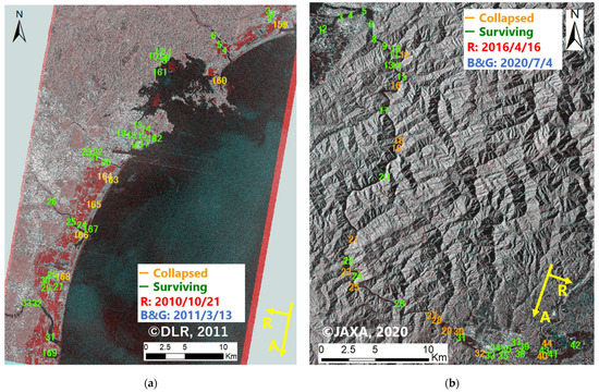
Figure 1.
Location of the 88 target bridges over the color composite of the pre-processed pre- and post-event SAR intensity images: (a) Seven collapsed and 34 surviving bridges affected by the 2011 Tohoku earthquake on the TerraSAR-X intensity pair, and (b) 14 collapsed and 30 surviving bridges affected by the 2020 July floods on the ALOS-2 intensity pair.

Table 1.
List of the collapsed bridges in the two target events under three damage conditions: (a) Part of the deck was washed away; (b) the deck was completely washed away, with piers left; and (c) the deck was completely washed away, without piers left [1,39].
2.2. Backscatter Model of Bridges
As multiple radar bounces occur between the water and the bridge, bridges over water have complicated backscatter patterns [22]. Backscatter models for bridges can be classified into two types, according to their heights [23,29]. Generally, a large-scale bridge with a high clearance over water is sturdy and difficult to collapse by floods or tsunamis. Thus, the damaged bridges were mainly small bridges with low clearance. Their backscatter model is shown in Figure 2. Layover (single-bounce), double-bounce, and triple-bounce patterns can be observed from the near-range to the far-range. When the height of the deck is not high enough, compared with the width of the deck, the triple-bounce overlaps on the layover. The length of layover () in the front of the outline in the ground range can be calculated using Equation (1), whereas the length of the triple-bounce () behind the outline can be calculated by Equation (2):
where is the clearance between the deck and water, and is the SAR incidence angle.
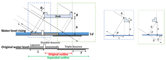
Figure 2.
Backscatter models of an over-water bridge under normal and high-water conditions.
To observe these signals clearly, an example of a low bridge in a high-resolution X-band airborne SAR intensity image is shown in Figure 3 [41]. It is an arch bridge over the Sumida River in Tokyo, Japan. The X-band airborne SAR sensor (Pi-SAR2) has 0.3 m resolution with full polarizations [42]. From the color composite of the HH, HV, and VV polarizations, we can observe the layover clearly as the white outline of the deck and arch. The purple signals consist of strong backscatter in the HH and VV polarizations, observed around the outline in the near-range, which are mainly the double-bounce backscattering from the side of the piers and the deck. Green signals with strong backscatter in the HV polarization can be observed from the middle of the bridge outline to the far-range, which are mainly due to triple-bounce backscattering.
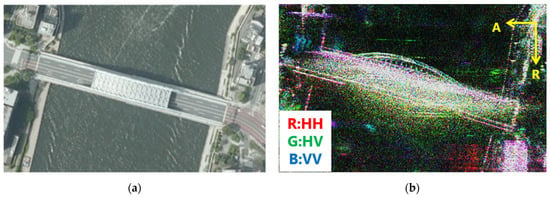
Figure 3.
An arch bridge over the Sumida River in Tokyo, Japan: (a) aerial photo taken by the Geospatial Information Authority of Japan [43]; (b) color composite of polarimetric Pi-SAR2 airborne SAR intensity image [42].
When the water level changes, the backscatter model of a bridge changes accordingly. Figure 2 also shows the model for an increased water level. As the distance between the sensor and the bridge does not change, the layover remains at the same location. However, the locations of the double- and triple-bounces move to the near-range. The movement of the double-bounce () can be described by Equation (3), and the movement of the triple-bounce is twice that of . Thus, the backscatter of the bridge will be seen differently after the water level rises.
where is the increase in the water level.
2.3. Extraction of Change Features
Five features obtained by the change detection method were used to build a classification model of collapsed bridges. These features were estimated within the outlines of bridges. According to the backscatter model in the previous section, we expanded the original outlines of bridges to include all of the backscatter signals. First, the original outlines were created from the GIS data of roads and rivers, which are available from the Geospatial Information Authority of Japan [44]. The roads over a water surface were extracted as the original outlines of bridges. The lengths of the bridges were defined as from bank to bank or nearest road to road. Then, we shifted the original outlines 10 m toward and away from the sensor direction. The expanded outlines were generated as the minimum rectangles including the original outline and two shifted outlines. According to the incident angles of the used SAR satellite images and Equations (1) and (2), the expanded outlines included the layover, double-bounce, and triple-bounce signals of the bridges lower than 7.6 m in both the TSX pairs and ALOS-2 pairs. Two examples of the original and expanded outlines in the pre-event TSX and ALOS-2 images are shown in Figure 4a,c.
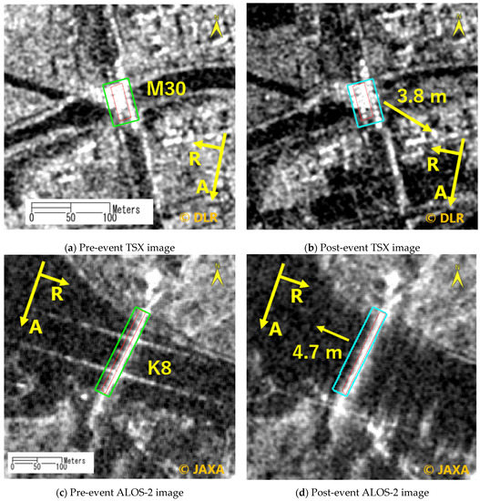
Figure 4.
Two examples of the original outline (red frame), the expanded outline (green frame), and the shifted outline (cyan frame) of the undamaged bridges: (a,b) bridge no. M30, with 3.8 m movement to the southeast direction due to an earthquake; and (c,d) bridge no. K8, with 4.7 m movement in the sensor direction due to a water level rise.
According to the backscatter model shown in Figure 3, the double-bounce and triple-bounce of the bridge moved in the sensor’s direction after the water level rose. If we conducted change detection directly, undamaged bridges would show similar features as damaged bridges. Thus, we shifted the expanded outlines of bridges in the post-event image to estimate the new location in the post-event SAR image [40]. In the Tohoku earthquake scenario, the flow observation stations located in the inundated area were all damaged by tsunamis. The increase in water level when the post-event SAR images were acquired was unknown, but it should be negligible two days after the tsunami. Furthermore, significant crustal movements occurred in the target area [45,46]. We shifted the expanded outlines in the eastern and southern directions, respectively. To increase accuracy, the SAR images were re-sampled to 0.25 m/pixel (i.e., one-fifth of the original products). In each shift of the sub-pixel step, the correlation of the backscatter intensity within the outlines was calculated. The location with the highest correlation was selected as the new outline in the post-event image.
In the July floods, three out of the six flow observation stations recorded an increase in water level at the peak that was more than 10 m. We also re-sampled the ALOS-2 images to 0.5 m/pixel (i.e., one-fifth of the original products). Then, shifting of the outline was conducted in the range direction, in a sub-pixel by sub-pixel manner. Two examples of the shifted outlines are shown in Figure 4b,d. Figure 4a,b show the pre- and post-event TSX images of an undamaged bridge (no. M30). Before the shifts, the correlation within the outline was 0.55. The correlation between the expanded outline in the pre-event image and the shifted outline in the post-event image increased to 0.85. Figure 4c,d are the pre- and post-event ALOS-2 images of an undamaged bridge (no. K8). After the shift of the outline, the correlation increased from 0.66 to 0.69. As the high water level at this location changed the backscatter pattern, the increase in the correlation was not significant, as was the case in the Tohoku earthquake scenario.
After modification of the outlines of bridges in the post-event SAR images, five features were calculated within the outlines from the multi-temporal SAR images. Correlation and differences were the most common features for the change direction. In a previous study, the correlation () was used to classify the bridges damaged in the Tohoku earthquake [28]. In this study, the correlation was also adopted as one of the change features. In the study [28], the correlation coefficient was calculated using a 3 ×3 pixel window. Then, the average value of the correlation within the outline was used for the classification step. However, we calculated the correlation using all the pixels within the outline in this study. Thus, only one correlation value was obtained for each bridge.
The difference was also adopted as an effective feature. We calculated the differences for each pixel within the outline of bridges. Then, the average value of the difference (), the standard deviation (), and the minimum value () were selected as three change features for the models. When the deck of a bridge has completely washed away, the backscatter within the outline might decrease significantly; however, sometimes, the average value of the difference does not change much when only a part of the deck is washed away. In addition, the remaining piers show high backscatter, reducing the change in the difference. Thus, we added the standard deviation and the minimum value of the difference, in order to improve the detection of partly washed-away bridges.
The last change feature was the percentage of the significantly changed area within the outline (). The purpose of introducing this feature was similar to the selection of the standard deviation and the minimum value of difference. Thresholding of the significantly changed area () was defined by subtracting twice the standard deviation from the average value of the difference for the whole scene. This thresholding method has been used to extract flooding areas where positive results were obtained in our previous studies [47,48].
A summary of these five change features is shown in Table 2, and the scattering plots in the two events are shown in Figure 5, respectively. Although the features of the target bridges in the two events were obtained from different SAR images with different wavelengths, their values and scattering patterns were similar. In the Tohoku earthquake, the surrounding environments of the target bridges changed significantly, due to the tsunami and its associated debris. The features of the surviving and collapsed bridges showed high variability. To the contrary, the features of the surviving bridges in the July floods had less variability. According to Figure 5, the collapsed bridges in the July floods could be identified easier than those after the Tohoku earthquake.
Table 2.
List of the five change features; where , are the pixels within the bridge outline in the pre- and post-event SAR images respectively, and means the average value.
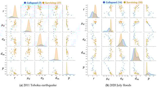
Figure 5.
Scatter plots of the five adopted change features of the target bridges affected in the 2011 Tohoku earthquake (a) and the 2020 July floods (b).
2.4. Generation of Data Sets
Two different data sets were generated for this study. The first data set used the features of bridges in one event, in order to train and test the model. Then, the model was applied to the features of the other event for verification. As the ratio of collapsed bridges in the July floods was larger than that after the Tohoku earthquake, we adopted this event to train the models. Fourteen collapsed bridges and 30 surviving bridges from the July floods were divided into training and test data randomly, with a ratio of 7:3. As a result, 11 collapsed bridges and 19 surviving bridges were used for training, while three collapsed bridges and 11 surviving bridges were used for testing. The seven collapsed bridges and 37 surviving bridges after the Tohoku earthquake were used as the validation set.
The second data set mixed all the features of the two events. First, the 88 target bridges were divided to two parts randomly, with a ratio of 7:3. The 30% was used for validation, including six collapsed bridges and 21 surviving bridges, while the 70% was divided again into training and test data randomly, with a ratio of 8:2. As a result, 10 collapsed bridges and 38 surviving bridges were used for training, while five collapsed bridges and eight surviving bridges were used for testing. The remaining six collapsed bridges and 21 surviving bridges were used as the validation set. The breakdown of the two data sets is shown in Table 3.
Table 3.
Numbers of bridges used in the two data sets.
3. Machine Learning Models
For this study, we adopted two common supervised algorithms to train and test the models. One is random forest (RF), an ensemble learning method for classification and regression [49]. Random forest builds multiple decision trees and merges them together to obtain an accurate and stable prediction. In this study, the input change features are selected randomly at each node to grow a decision tree. Then each tree casts a unit vote for the most popular class to classify bridges. The other one is logistic regression (LR), a reliable procedure to solve binary classification problems [36]. The core of logistic regression is the “S”-shaped logistic function. The curve of the logistic function indicates the likelihood of the target class. Using the two data sets and the two machine learning methods, twelve models were generated, with different numbers of input features.
3.1. Models Using Data Set 1
First, RF and LR models were trained and tested using data set 1. To determine the optimal values for the models, hyperparameter tuning was conducted, using the GridSearchCV function of the Python package scikit-learn [50]. For the RF models, the best combination of the three hyperparameters were examined: n_estimators, max_depth, and random_state. “n_estimators” is the number of trees in the model, which was pre-defined as 5, 10, 30, and 50. “max_depth” is the maximum depth of the tree, which was pre-defined as 3, 5, 10, 30, and 50. “random_state” controls both the randomness of bootstrapping for the samples to build trees and the sampling of the features to consider the best split at each node, which was predefined as 0, 7, and 42. As the number of bridges in the training data was limited, we performed three-fold cross-validation, in order to obtain the best combination of hyperparameters.
For the first try, the five change features obtained in the previous section were all used for fitting. Fitting of the RF model was conducted using the abovementioned function of scikit-learn [50]. As a result, 10 out of 11 collapsed bridges in the training data and 2 out of 3 collapsed bridges in the test data were detected successfully. In addition, no surviving bridge was detected as a commission error. According to the impurity-based feature importance obtained after fitting, we deleted the feature , as it had the lowest importance value. Then, fitting was conducted again, using the remaining four features. As a result, all the collapsed bridges in the training data and two collapsed bridges in the test data were detected without a commission error. Finally, the feature , with the lowest importance value, was also removed from the input. Fitting was then conducted using the features , , and . The result was the same as that with the model using all five features.
A comparison of the three RF models using different numbers of features is shown in Table 4. Four indices were used to evaluate the performance of the models: the recall and precision of the collapsed bridges, the accuracy, and the kappa coefficient. In this study, the collapsed class was set as positive. A high recall means the collapsed bridges were detected successfully, and a high precision means the surviving bridges were not misidentified as collapsed. Since there were three times more surviving bridges than collapsed bridges, we adopted the kappa coefficient to describe the performance of the models.
Table 4.
Comparison of the RF models using data set 1 with different numbers of features, where the best model is emphasized in bold font. The highest accuracy for the test data is emphasized by the gray background.
According to Table 4, the RF models using different numbers of features obtained the same results on the test data. As the model using four features had higher accuracy on the training set, this model was applied to the Tohoku earthquake validation set. The confusion matrix is shown in Table 5. Five out of seven collapsed bridges were detected successfully, but 12 surviving bridges were misclassified as collapsed. The kappa coefficient was 0.25, showing only fair agreement.
Table 5.
Confusion matrix of the validation set using the RF model with three input features.
For the LR models, the best combination of two hyperparameters was examined: C and random_state. “C” is the inverse of regularization strength, wherein smaller values specify stronger regularization. “random_state” is the same as that in the RF models. “C” was pre-defined as , where is an integer from −5 to 6. “random_state” was pre-defined as an integer from 0 to 101. The hyperparameters were tuned by three-fold cross-validation. The threshold value of the logistic function was set as 0.5. Firstly, the LR models were fed the five features. Seven out of 11 collapsed bridges in the training set and two out of three collapsed bridges in the test set were detected successfully, without a commission error. The feature was deleted, due to its high p-value. The new LR model, using four features, detected nine collapsed bridges in the training set and three collapsed bridges in the test set; meanwhile, one surviving bridge in the training set and one in the test set were misclassified. The third LR model, using the three features , , and with the lowest p-values of the five features, was then considered. The result was the same as that using the four features. Considering that less processing time is taken when using fewer features, the LR model with three features was adopted for verification. A comparison of the three LR models is shown in Table 6. The confusion matrix for the validation set is shown in Table 7. Five out of seven collapsed bridges were detected, whereas 10 surviving bridges were misclassified. This result was better than that obtained with the RF model, although the kappa coefficient was still low (0.3).
Table 6.
Comparison of the LR models using data set 1 with different numbers of features, where the best model is emphasized in bold font. The highest accuracy for the test set is emphasized by the gray background.
Table 7.
Confusion matrix of the validation set using the LR model with three input features.
Comparing the results with those using data set 1, the RF models obtained a better accuracy for the training set, whereas the LR models obtained better results on the test set. Although all the models obtained substantial agreement with the test set, they had difficulty with the validation set, which consisted of the damage data set for the other event. The LR model using the three features—namely, , , and —was the best model when fitted with data set 1. Using this model, 12 out of 14 collapsed bridges were detected for the July floods, and five out of seven collapsed bridges were detected for the Tohoku earthquake. The omitted collapsed bridges were K23, K30, M163, and M164. For all of the target bridges, the recall of the collapsed bridges was 0.81 and the precision was 0.59. The accuracy was 0.82 and the kappa coefficient was 0.56, showing only a moderate level of agreement.
3.2. Models Using the Dataset 2
Next, the fitting of the RF and LR models using data set 2 was conducted. The hyperparameters were pre-defined using the same values as those for data set 1. Hyperparameter tuning was carried out using the training and test sets. Then, the best combination of hyperparameters was applied to each model. Examination of the features was also carried out, by reducing the number of input data. Comparisons of the RF and LR models are shown in Table 8 and Table 9, respectively. For the LR models, the threshold value of the logistic function was also set as 0.5.
Table 8.
Comparison of RF models using data set 2 with different numbers of features; the best model is emphasized in bold font. The highest accuracy for the test data is emphasized by the gray background.
Table 9.
Comparison of the LR models using data set 2 with the different numbers of features; the best model is emphasized in bold font. The highest accuracy for the test data is emphasized by the gray background.
For the training set, the RF model using all the features and the one using four features obtained the same results, wherein seven out of 10 collapsed bridges were successfully identified. The model using three features detected six collapsed bridges, worse than the other models. For the test set, the models using all the features classified three out of five collapsed bridges, better than the other two models. Thus, the RF model using all five features showed the best discrimination ability for data set 2. These models were applied to the validation set. Five out of six collapsed bridges were detected by the best RF model and the model using the three features (, , and ). Only one surviving bridge (K31) was misclassified as collapsed.
As the validation set was selected from the target bridges randomly, we changed the division of the validation sets 10 times to improve the reliability. Then, the RF model using all the features was applied to those validation sets. The best discrimination result was obtained for the validation set, including four collapsed bridges and 23 surviving bridges, wherein all the bridges were successfully classified. The worst result identified two out of five collapsed bridges and 22 surviving bridges. The recall of the collapsed bridges was 0.40, and the accuracy was 0.89. The kappa coefficient of the worst result was 0.52, showing moderate agreement. The RF model for the other nine validation sets had higher kappa coefficients than 0.60, indicating substantial agreement. The average values of the evaluation indices were used as the final accuracy of the best model. The recall of the collapsed bridges was 0.71, and the precision was 0.94. The accuracy was 0.91, and the kappa coefficient was 0.74.
For the LR models, three models using different numbers of features obtained the same results. Five out of 10 collapsed bridges in the training set and three out of five collapsed bridges in the test set were detected. No surviving bridges were misclassified as collapsed. For the validation set, these models also obtained the same results, wherein four out of six collapsed bridges were detected successfully and one surviving bridge was misclassified. Considering the number of features, we applied the LR model using the three features , , and to 10 random validation sets. The best discrimination result was obtained for the validation set including four collapsed bridges and 23 surviving bridges, wherein all the bridges were successfully classified. The worst result identified two out of five collapsed bridges and 21 out of 22 surviving bridges. The recall of the collapsed bridges was 0.40, and the accuracy was 0.85. The kappa coefficient of the worst result was 0.42, showing moderate agreement. The LR model, for four out of the 10 validation sets, had a kappa coefficient lower than 0.6, while it showed a kappa coefficient higher than 0.8 for only one of the validation sets, which gave the best accuracy. The average value of the recall was 0.70, and the precision was 0.89. The accuracy was 0.88, and the kappa coefficient was 0.62. This accuracy was worse than that of the RF model using all the features. Thus, the RF model using the five features was the best model when fitted using data set 2.
Using the best RF model, 11 out of 14 collapsed bridges were detected for the July floods, and four out of seven collapsed bridges were detected for the Tohoku earthquake, respectively. The omitted collapsed bridges were K21, K23, K30, M160, M163, and M168. The only misclassified surviving bridge was K31. For all the target bridges, the recall of the collapsed bridges was 0.71, and the precision was 0.94. The accuracy was 0.92, and the kappa coefficient was 0.76, indicating substantial agreement.
3.3. Comparison and Improvement of the Models
According to a comparison of the RF models and LR models using different numbers of features, the LR model using the features , , and was the best model when fitted by data set 1, whereas the RF model using all the features was the best when fitted by data set 2. The LR model with three features obtained high accuracy for the test data where the recall was 1.00 and the kappa coefficient was 0.81; however, this model had difficulty in classifying the collapsed bridges in the other event. The RF model trained using the collapsed bridges from both events identified more than 60% of collapsed bridges in the training and test data. It obtained high accuracy in the validation data. Considering the high kappa coefficient in the validation, the RF model using all the change features (i.e., , ,, ) was the best of the twelve proposed models.
The pre- and post-event TSX intensity images and the post-event aerial photos taken by the GSI [43] for the collapsed bridges M160, M163, and M168 are shown in Figure 6. These bridges could not be identified, even by the best RF model. From the aerial photos of the bridges M160 and M163, we recognized that only part of the deck was washed away. The changed regions were limited, compared with the whole bridges. Thus, they were difficult to identify. The bridge M168 was a small bridge, 16.8 m in length and 3.7 m in width [1]. As the spatial resolution of the TSX images is about 3 m, the reflection region from the bridge was very small. Although the whole deck was washed away, it was still difficult to identify.
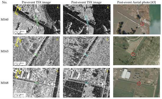
Figure 6.
Three partly collapsed or washed-away bridges that could not be identified by the best RF model using five features for the data set 2 [43].
The pre- and post-event TSX intensity images and the post-event ground photos of the collapsed bridges K23 and K30 are shown in Figure 7. They were not identified by the best RF model. One surviving bridges, K31, which was misclassified as collapsed is also shown in Figure 7. The ground photos were taken by one of the co-authors on Sept. 17, 2020. Bridge K23, which was located at the radar shadow of mountains, had weak backscatter in the pre-event ALOS-2 image. Although the deck was completely washed away, the change in the intensity images was slight. Thus, it was classified as surviving. The collapsed bridge K21 was omitted for the same reason. Bridge K30 was a partly collapsed old bridge. One span of the deck, connecting to the embankment, had failed. The collapsed part was narrow and close to the land; hence, it was missed by the model. Bridge K31 was the only surviving bridge classified as collapsed. According to the ground photo, there was no significant damage. However, the backscatter patterns of the pre- and post-event intensity images were different. This change was caused by two reasons, at the time of the post-event ALOS-2 image acquisition. One was the flooding over the embankment, which reduced the backscatter from the east part of the outline. The other reason is the high water level. The water level increased close to the deck, which reduced the backscatter of the double- and triple-bounces. It is quite a rare case that a SAR image is obtained under flooding conditions.
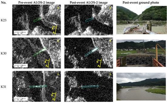
Figure 7.
Two collapsed bridges, K23 and K30, that could not be identified by the RF model using five features for data set 2, and one surviving bridge, K31, which was misclassified as collapsed.
The RF model using the five change features of data set 2 showed good capability for the detection of collapsed bridges, with a kappa coefficient of 0.76. As our objective is the detection of collapsed bridges, a recall accuracy of 0.71 is still not enough. Thus, we introduced an oversampling technique to improve the model. The synthetic minority over-sample technique (SMOTE) is an oversampling approach to create synthetic examples for the minority class [51]. There were 10 collapsed bridges and 38 surviving bridges in the training set of data set 2. We used the SMOTE function in the Imbalanced-learn library to increase the number of collapsed bridges to 38, the same as the number of surviving bridges in the training set [52]. Then, the RF model was trained using the five features from the 76 samples.
The accuracies of the results are shown in Table 10. The kappa coefficient for the training set decreased from 0.79 to 0.75, whereas it increased from 0.65 to 0.68 for the test set. For the training set, eight out of 10 collapsed bridges were identified successfully, with two misclassified surviving bridges. For the test set, four out of five collapsed bridges were detected, whereas one surviving bridge was misclassified. For the validation set, all six collapsed bridges were identified, and two surviving ones were misclassified as collapsed. The recall of the collapsed bridges reached 1.0. The obtained model was applied to 10 validation sets, which were divided randomly. The minimum recall was 0.80, and the minimum kappa coefficient was 0.70, representing better accuracy than the original RF model. The final recall of the validation set was 0.96, and the precision was 0.80. The accuracy was 0.93, and the kappa coefficient was 0.82, indicating almost perfect agreement.
Table 10.
The accuracies of the RF model using five features after applying the SMOTE technique.
Using the modified RF model, 13 out of 14 collapsed bridges were detected in the July floods event, and five out of seven collapsed bridges were detected in the Tohoku earthquake. The omission errors for collapsed bridges were K30, M160, and M163. The misclassified surviving bridges increased, being K3, K31, K38, M10, and M16. For all the target bridges, the recall of the collapsed bridges was 0.95, and the precision was 0.80. The accuracy was 0.93, and the kappa coefficient was 0.82, indicating substantial agreement. Therefore, this model showed sufficient capability for the detection of collapsed bridges.
We applied the random forest and logistic regression methods to two different data sets. When fitting with data set 1, the RF models using four features and the LR models using three features obtained the best results. The RF models showed better accuracy in the training step; however, their accuracies in the test step were lower than those of the LR models. When fitting with data set 2, the RF model using five features obtained the best accuracy, whereas all the LR models obtained the same results, regardless of input features. The accuracy of the test data using data set 1 was better than that using data set 2. On the contrary, the accuracy of validation using data set 2 was better than that using data set 1. The training and test data of data set 1 were from one event—the July floods. The variation in damage patterns and surrounding environment was small, which led to good accuracy in the training and test steps. When those models were applied to the other event—that is, the Tohoku earthquake—their accuracy decreased significantly. For the models trained using the mixed data from the two events (data set 2), the accuracies in the fitting approach were moderate. However, the models have more versatility, which led to better validation accuracy. According to these comparisons, we can summarize the characteristics of the models as follows: (1) when the training data were limited, the LR model with a few features showed a good capability to describe the data; (2) the FR models had more capability for the various data sets; and (3) the increase in diversity in the training data improved the performance of the model.
After applying the oversampling approach to the training data for data set 2, the recall, accuracy, and kappa coefficient of the RF model increased. Only the partially collapsed bridge, M30, which was affected by the July floods, could not be identified. Further, the commission error increased from one to five bridges, including two bridges affected by the July floods and three bridges affected by the Tohoku earthquake. Comparing the importance of the five features in the RF model and the modified RF model, the third important feature changed from the correlation in the RF model to the average of difference in the modified RF model. This might be the reason for the improvement in the recall accuracy. The modified RF model showed very high capability for detecting collapsed bridges.
In the previous study [28], the thresholding of correlation coefficient was used to detect severely damaged bridges for the Tohoku earthquake. The threshold value was defined by a statistic discussion. The recall of the severely damaged bridges was 89%, and the kappa coefficient was only 0.43. Comparing to the result in [28], the best model in this study achieved 95% recall and 0.82 kappa coefficient, showing significant improvement. In additional, the thresholding method needs manual definition of the threshold value, whereas the proposed model classifies bridges automatedly.
There were two limitations to the proposed models. First, the outlines of bridges were necessary. In this study, we created the original outlines using GIS data of roads and rivers. When GIS data are not available, it is difficult to generate bridge outlines. The detection of bridges using a deep learning method could provide a solution to this problem [26]. Another limitation is that both pre- and post-event SAR images acquired under the same conditions are required; however, pre-event SAR images are not always available. On the contrary, the proposed method can be applied to different SAR pairs, even with different wavelength. As the features were obtained according to the changes, the influence of the acquisition conditions and sensors was reduced. Thus, we could improve our model by combining more damaged bridges from different events using different SAR sensors.
4. Conclusions
In this study, we used random forest and logistic regression methods to identify collapsed bridges. Two data sets were generated, using the change features from 88 affected bridges in the 2011 Tohoku-oki earthquake and the 2020 July floods, both in Japan. The first data set included training and test data from one event, and validation data from another event. The second data set included mixed data from the two events, which were divided into training, test, and validation data randomly. The input data of the models were five features determined by the change detection step. After a comparison of different numbers of input features, the random forest model using five features for data set 2 showed the best validation accuracy. Fifteen out of 21 collapsed bridges were identified successfully, with one misclassified surviving bridge. Then, an oversampling approach was introduced to the training data to balance the number of samples for the two classes. The new model, trained by the modified training data, could identify more collapsed bridges, showing almost perfect agreement with the true data. In the future, we intend to keep collecting the data of damaged bridges to improve the versatility of the RF model.
Author Contributions
Conceptualization, W.L.; Data curation, F.Y.; Formal analysis, W.L.; Funding acquisition, F.Y.; Investigation, W.L. and F.Y.; Methodology, W.L. and Y.M.; Project administration, Y.M.; Validation, W.L.; Writing—original draft, W.L.; Writing—review and editing, Y.M. and F.Y. All authors have read and agreed to the published version of the manuscript.
Funding
This research was funded by JSPS KAKENHI, grant number 21H01598.
Acknowledgments
The TerraSAR-X images used in this study are the property of DLR and distributed by Airbus DS/Infoterra GmbH. The ALOS-2 PALSAR-2 data used in this study are owned by the Japan Aerospace Exploration Agency (JAXA) and were provided for the ALOS-2 research program (RA6, PI No.3243). The Pi-SAR2 images used in this study are owned by the National Institute of Information and Communications Technology (NICT), Japan, and were made available through the collaborative research between NICT and Chiba University.
Conflicts of Interest
The authors declare no conflict of interest.
References
- National Institute for Land and Infrastructure Management (NILM). Annual Report of Road-Related Research in FY 2013. Technical Note of NILIM 2013, No. 843. pp. 3–110. Available online: http://www.nilim.go.jp/lab/bcg/siryou/tnn/tnn0843.htm (accessed on 1 July 2021).
- Japan Bridge Association Inc. Investigation Report of Bridge Damages in the Kumamoto Earthquake. Available online: https://www.jasbc.or.jp/whatsnew/files/161227/kyoryohigaityousahoukokusyo.pdf (accessed on 1 July 2021). (In Japanese).
- Tanabe, R.; Yamazaki, F.; Liu, W. Damage analysis of landslides and bridges in Minami-Aso village due to 2016 Kumamoto earthquake using full-polarimetric airborne SAR images. In Proceedings of the 39th Asian Conference on Remote Sensing, Kuala Lumpur, Malaysia, 15–19 October 2018; pp. 1545–1553. [Google Scholar]
- Joyce, K.E.; Belliss, S.E.; Samsonov, S.V.; McNeill, S.J.; Glassey, P.J. A review of the status of satellite remote sensing and image processing techniques for mapping natural hazards and disasters. Prog. Phys. Geogr. Earth Environ. 2009, 33, 183–207. [Google Scholar] [CrossRef]
- Dell’Acqua, F.; Gamba, P. Remote Sensing and Earthquake Damage Assessment: Experiences, Limits, and Perspectives. Proc. IEEE 2012, 100, 2876–2890. [Google Scholar] [CrossRef]
- Lin, L.; Di, L.; Yu, E.G.; Kang, L.; Shrestha, R.; Rahman, S.; Tang, J.; Deng, M.; Sun, Z.; Zhang, C.; et al. A review of remote sensing in flood assessment. In Proceedings of the 2016 Fifth International Conference on Agro-Geoinformatics (Agro-Geoinformatics), Tianjin, China, 18–20 July 2016; Volume 16373607, pp. 1–4. [Google Scholar]
- Koshimura, S.; Moya, L.; Mas, E.; Bai, Y. Tsunami Damage Detection with Remote Sensing: A Review. Geosciences 2020, 10, 177. [Google Scholar] [CrossRef]
- Saito, K.; Spence, R.J.S.; Going, C.; Markus, M. Using High-Resolution Satellite Images for Post-Earthquake Building Damage Assessment: A Study following the 26 January 2001 Gujarat Earthquake. Earthq. Spectra 2004, 20, 145–169. [Google Scholar] [CrossRef]
- Miura, H.; Midorikawa, S.; Kerle, N. Detection of Building Damage Areas of the 2006 Central Java, Indonesia, Earthquake through Digital Analysis of Optical Satellite Images. Earthq. Spectra 2013, 29, 453–473. [Google Scholar] [CrossRef]
- Janalipour, M.; Mohammadzadeh, A. A Fuzzy-GA Based Decision Making System for Detecting Damaged Buildings from High-Spatial Resolution Optical Images. Remote Sens. 2017, 9, 349. [Google Scholar] [CrossRef]
- Adriano, B.; Xia, J.; Baier, G.; Yokoya, N.; Koshimura, S. Multi-Source Data Fusion Based on Ensemble Learning for Rapid Building Damage Mapping during the 2018 Sulawesi Earthquake and Tsunami in Palu, Indonesia. Remote Sens. 2019, 11, 886. [Google Scholar] [CrossRef]
- Balz, T.; Perissin, D.; Soergel, U.; Zhang, L.; Liao, M. Post-seismic infrastructure damage assessment using high-resolution SAR satellite data. Proceedings of the 2nd International Conference on Earth Observation for Global Change. 2009. Available online: https://engineering.purdue.edu/~perissin/Publish/09EOGC_hres.pdf (accessed on 1 July 2021).
- Chen, F.; Lin, H.; Li, Z.; Chen, Q.; Zhou, J. Interaction between permafrost and infrastructure along the Qinghai–Tibet Railway detected via jointly analysis of C- and L-band small baseline SAR interferometry. Remote Sens. Environ. 2012, 123, 532–540. [Google Scholar] [CrossRef]
- Lu, H.; Zhang, H.; Deng, Y.; Wang, J.; Yu, W. Building 3-D Reconstruction With a Small Data Stack Using SAR Tomography. IEEE J. Sel. Top. Appl. Earth Obs. Remote Sens. 2020, 13, 2461–2474. [Google Scholar] [CrossRef]
- Balz, T.; Liao, M. Building-damage detection using post-seismic high-resolution SAR satellite data. Int. J. Remote Sens. 2010, 31, 3369–3391. [Google Scholar] [CrossRef]
- Plank, S. Rapid Damage Assessment by Means of Multi-Temporal SAR—A Comprehensive Review and Outlook to Sentinel-1. Remote Sens. 2014, 6, 4870–4906. [Google Scholar] [CrossRef]
- Nie, Y.; Zeng, Q.; Zhang, H.; Wang, Q. Building Damage Detection Based on OPCE Matching Algorithm Using a Single Post-Event PolSAR Data. Remote Sens. 2021, 13, 1146. [Google Scholar] [CrossRef]
- Ge, P.; Gokon, H.; Meguro, K. A review on synthetic aperture radar-based building damage assessment in disasters. Remote Sens. Environ. 2020, 240, 111693. [Google Scholar] [CrossRef]
- Adriano, B.; Yokoya, N.; Xia, J.; Miura, H.; Liu, W.; Matsuoka, M.; Koshimura, S. Learning from multimodal and multitemporal earth observation data for building damage mapping. ISPRS J. Photogramm. Remote Sens. 2021, 175, 132–143. [Google Scholar] [CrossRef]
- Abdi, G.; Jabari, S. A Multi-Feature Fusion Using Deep Transfer Learning for Earthquake Building Damage Detection. Can. J. Remote Sens. 2021, 47, 1–16. [Google Scholar] [CrossRef]
- Wang, Y.; Zheng, Q. Recognition of roads and bridges in SAR images. Pattern Recognit. 1998, 31, 953–962. [Google Scholar] [CrossRef]
- Soergel, U.; Cadario, E.; Thiele, A.; Thoennessen, U. Extraction of bridges over water in multi-aspect high-resolution InSAR data. In Proceedings of the Symposium of ISPRS Comission III Photogrametric Computer Vision PCV’ 06, Bonn, Germany, 20–22 September 2006; Available online: https://www.isprs.org/proceedings/XXXVI/part3/singlepapers/P_17.pdf (accessed on 1 July 2021).
- Liu, W.; Sawa, K.; Yamazaki, F. Backscattering characteristics of bridges from high-resolution X-band SAR imagery. In Proceedings of the International Symposium on Remote Sensing 2017, Nagoya, Japan, 17–19 May 2017; pp. 324–327. [Google Scholar]
- Cadario, E.; Gross, H.; Hammer, H.; Schulz, K.; Thiele, A.; Thoennessen, U.; Soergel, U.; Weydahl, D.J. Change Detection for Bridges over Water in Airborne and Spaceborne SAR Data. In Proceedings of the IGARSS 2008 IEEE International Geoscience and Remote Sensing Symposium, Boston, MA, USA, 7–11 July 2008; Volume 5, pp. 479–482. [Google Scholar] [CrossRef]
- Yang, M.; Jian, Z. Bridge detection in high-resolution X-band SAR images by combined statistical and topological approach. Prog. Electromagn. Res. M 2017, 57, 91–102. [Google Scholar] [CrossRef][Green Version]
- Chen, L.; Weng, T.; Xing, J.; Pan, Z.; Yuan, Z.; Xing, X.; Zhang, P. A New Deep Learning Network for Automatic Bridge Detection from SAR Images Based on Balanced and Attention Mechanism. Remote Sens. 2020, 12, 441. [Google Scholar] [CrossRef]
- Jiang, K.; Wang, C.; Zhang, H.; Chen, W.; Zhang, B.; Tang, Y.; Wu, F. Damage analysis of 2008 Wenchuan earthquake using SAR images. In Proceedings of the 2009 IEEE International Geoscience and Remote Sensing Symposium, Cape Town, South Africa, 12–17 July 2019. [Google Scholar] [CrossRef]
- Inoue, K.; Liu, W.; Yamazaki, F. Detection of Bridge Damages due to Tsunami Using Multi-temporal High-resolution SAR Images. J. Jpn. Assoc. Earthq. Eng. 2017, 17, 5. [Google Scholar] [CrossRef][Green Version]
- Liu, W.; Yamazaki, F. Extraction of Collapsed Bridges Due to the 2011 Tohoku-Oki Earthquake from Post-Event SAR Images. J. Disaster Res. 2018, 13, 281–290. [Google Scholar] [CrossRef]
- Liu, W.; Yamazaki, F. Bridge damage assessment using single post-event TerraSAR-X image. In Proceedings of the IEEE 2019 International Geoscience and Remote Sensing Symposium, Yokohama, Japan, 28 July–2 August 2019; pp. 4833–4836. [Google Scholar] [CrossRef]
- Sester, M.; Feng, Y.; Thiemann, F. Building generalization using deep learning. ISPRS-Int. Arch. Photogramm. Remote Sens. Spat. Inf. Sci. 2018, XLII-4, 565–572. [Google Scholar] [CrossRef]
- Zhang, X.; Liu, G.; Zhang, C.; Atkinson, P.M.; Tan, X.; Jian, X.; Zhou, X.; Li, Y. Two-Phase Object-Based Deep Learning for Multi-Temporal SAR Image Change Detection. Remote Sens. 2020, 12, 548. [Google Scholar] [CrossRef]
- Derksen, D.; Inglada, J.; Michel, J. Geometry Aware Evaluation of Handcrafted Superpixel-Based Features and Convolutional Neural Networks for Land Cover Mapping Using Satellite Imagery. Remote Sens. 2020, 12, 513. [Google Scholar] [CrossRef]
- Belgiu, M.; Drăguţ, L. Random forest in remote sensing: A review of applications and future directions. ISPRS J. Photogramm. Remote Sens. 2016, 114, 24–31. [Google Scholar] [CrossRef]
- Bioucas-Dias, J.M.; Plaza, A.; Camps-Valls, G.; Scheunders, P.; Nasrabadi, N.; Chanussot, J. Hyperspectral Remote Sensing Data Analysis and Future Challenges. IEEE Geosci. Remote Sens. Mag. 2013, 1, 6–36. [Google Scholar] [CrossRef]
- Ray, S. A quick review of machine learning algorithms. In Proceedings of the 2019 International Conference on Machine Learning, Big Data, Cloud and Parallel Computing (Com-IT-Con), Faridabad, India, 14–16 February 2019; pp. 35–39. [Google Scholar] [CrossRef]
- Shoji, G.; Nakamura, T. Damage Assessment of Road Bridges Subjected to the 2011 Tohoku Pacific Earthquake Tsunami. J. Disaster Res. 2017, 12, 79–89. [Google Scholar] [CrossRef]
- Japan Weather Association. Characteristics of rainfall in Kumamoto Heavy Rain and Future Outlook (Flash Report). Disaster Report. 2020. Available online: https://www.jwa.or.jp/news/2020/07/10378/ (accessed on 1 July 2021). (In Japanese).
- Cabinet Office, Government of Japan. Report of the Damage Situation Related to 14:00 on 2 November 2020. Available online: http://www.bousai.go.jp/updates/r2_07ooame/pdf/r20703_ooame_38.pdf (accessed on 1 July 2021). (In Japanese)
- Liu, W.; Maruyama, Y.; Yamazaki, F. Damage assessment of bridges due to the 2020 July Flood in Japan using ALOS-2 intensity images. In Proceedings of the IEEE 2021 International Geoscience and Remote Sensing Symposium, Online, 12–16 July 2021. [Google Scholar]
- Hirano, H.; Yamazaki, F.; Liu, W. Backscattering characteristics of bridges from airborne full-polarimetric SAR images. In Proceedings of the 38th Asian Conference on Remote Sensing, New Delhi, India, 23–27 October 2017. [Google Scholar]
- National Institute of Information and Communications Technology (NICT). Available online: https://www.nict.go.jp/out-promotion/other/case-studies/itenweb/Pi-sar2.html (accessed on 1 July 2021). (In Japanese).
- Geospatial Information Authority of Japan (GSI). Digital Map of Japan. Available online: https://maps.gsi.go.jp (accessed on 1 July 2021). (In Japanese)
- Geospatial Information Authority of Japan (GSI). Fundamental Geospatial Data. Available online: https://www.gsi.go.jp/kiban/ (accessed on 1 July 2021). (In Japanese)
- Liu, W.; Yamazaki, F. Detection of Crustal Movement From TerraSAR-X Intensity Images for the 2011 Tohoku, Japan Earthquake. IEEE Geosci. Remote Sens. Lett. 2012, 10, 199–203. [Google Scholar] [CrossRef]
- Liu, W.; Yamazaki, F.; Matsuoka, M.; Nonaka, T.; Sasagawa, T. Estimation of three-dimensional crustal movements in the 2011 Tohoku-Oki, Japan, earthquake from TerraSAR-X intensity images. Nat. Hazards Earth Syst. Sci. 2015, 15, 637–645. [Google Scholar] [CrossRef]
- Liu, W.; Yamazaki, F. Review article: Detection of inundation areas due to the 2015 Kanto and Tohoku torrential rain in Japan based on multi-temporal ALOS-2 imagery. Nat. Hazards Earth Syst. Sci. 2018, 18, 1905–1918. [Google Scholar] [CrossRef]
- Liu, W.; Fujii, K.; Maruyama, Y.; Yamazaki, F. Inundation Assessment of the 2019 Typhoon Hagibis in Japan Using Multi-Temporal Sentinel-1 Intensity Images. Remote Sens. 2021, 13, 639. [Google Scholar] [CrossRef]
- Liaw, A.; Wiener, M. Classification and Regression by randomForest. R News 2002, 2, 18–22. [Google Scholar]
- Scikit-Learn Developers. Scikit-Learn. Retrieved October 2020. 2020. Available online: https://scikit-learn.org/stable/index.html (accessed on 1 July 2021).
- Chawla, N.V.; Bowyer, K.W.; Hall, L.O.; Kegelmeyer, W.P. SMOTE: Synthetic Minority Over-sampling Technique. J. Artif. Intell. Res. 2002, 16, 321–357. [Google Scholar] [CrossRef]
- Imbalanced-Learn Documentation. Available online: https://imbalanced-learn.org/stable/# (accessed on 1 July 2021).


Publisher’s Note: MDPI stays neutral with regard to jurisdictional claims in published maps and institutional affiliations. |
© 2021 by the authors. Licensee MDPI, Basel, Switzerland. This article is an open access article distributed under the terms and conditions of the Creative Commons Attribution (CC BY) license (https://creativecommons.org/licenses/by/4.0/).