
On the Generalization Ability of a Global Model for Rapid Building Mapping from Heterogeneous Satellite Images of Multiple Natural Disaster Scenarios


Abstract
1. Introduction
2. Evaluation
2.1. xBD Dataset
2.1.1. Images in the xBD Dataset
2.1.2. Damage Scales in xBD Dataset
2.1.3. Quality of the xBD Dataset
2.1.4. Differences between Disasters
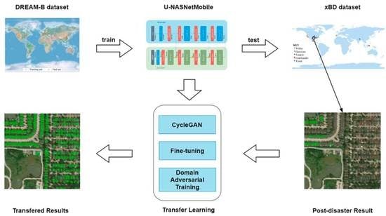
2.2. The Global Model Trained on DREAM-B
2.2.1. DREAM-B Dataset
2.2.2. U-NASNetMobile
2.3. Evaluation
3. Promotion
3.1. Fine-Tuning
3.1.1. Fine-Tuning Using Images from xBD
3.1.2. Quantitative Evaluation
3.1.3. Qualitative Comparison
3.2. CycleGAN
3.2.1. Image Translation from xBD to DREAM-B
3.2.2. Quantitative Evaluation
3.2.3. Qualitative Comparison
3.3. Domain Adversarial Training
3.3.1. Domain Adversarial Training between xBD and DREAM-B
3.3.2. Quantitative Evaluation
3.3.3. Qualitative Comparison
4. Discussion
5. Conclusions
Author Contributions
Funding
Institutional Review Board Statement
Informed Consent Statement
Acknowledgments
Conflicts of Interest
References
- Dong, L.; Shan, J. A comprehensive review of earthquake-induced building damage detection with remote sensing techniques. ISPRS J. Photogramm. Remote Sens. 2013, 84, 85–99. [Google Scholar] [CrossRef]
- Tomowski, D.; Klonus, S.; Ehlers, M.; Michel, U.; Reinartz, P. Change visualization through a texture-based analysis approach for disaster applications. In Proceedings of the ISPRS Proceedings, Vienna, Austria, 5–7 July 2010; pp. 1–6. [Google Scholar]
- Miura, H.; Modorikawa, S.; Chen, S.H. Texture characteristics of high-resolution satellite images in damaged areas of the 2010 Haiti earthquake. In Proceedings of the 9th International Workshop on Remote Sensing for Disaster Response, Stanford, CA, USA, 15–16 September 2011; pp. 15–16. [Google Scholar]
- Chini, M.; Cinti, F.; Stramondo, S. Co-seismic surface effects from very high resolution panchromatic images: The case of the 2005 Kashmir (Pakistan) earthquake. Nat. Hazards Earth Syst. Sci. 2011, 11, 931–943. [Google Scholar] [CrossRef]
- Zhao, F.; Zhang, C. Building Damage Evaluation from Satellite Imagery using Deep Learning. In Proceedings of the 2020 IEEE 21st International Conference on Information Reuse and Integration for Data Science (IRI), Las Vegas, NV, USA, 11–13 August 2020; pp. 82–89. [Google Scholar]
- Kalantar, B.; Ueda, N.; Al-Najjar, H.A.; Halin, A.A. Assessment of Convolutional Neural Network Architectures for Earthquake-Induced Building Damage Detection based on Pre-and Post-Event Orthophoto Images. Remote Sens. 2020, 12, 3529. [Google Scholar] [CrossRef]
- Ma, J.; Qin, S. Automatic depicting algorithm of earthquake collapsed buildings with airborne high resolution image. In Proceedings of the 2012 IEEE International Geoscience and Remote Sensing Symposium, Munich, Germany, 22–27 July 2012; pp. 939–942. [Google Scholar]
- Ci, T.; Liu, Z.; Wang, Y. Assessment of the Degree of Building Damage Caused by Disaster Using Convolutional Neural Networks in Combination with Ordinal Regression. Remote Sens. 2019, 11, 2858. [Google Scholar] [CrossRef]
- Miura, H.; Aridome, T.; Matsuoka, M. Deep learning-based identification of collapsed, non-collapsed and blue tarp-covered buildings from post-disaster aerial images. Remote Sens. 2020, 12, 1924. [Google Scholar] [CrossRef]
- Valentijn, T.; Margutti, J.; Van den Homberg, M.; Laaksonen, J. Multi-hazard and spatial transferability of a cnn for automated building damage assessment. Remote Sens. 2020, 12, 2839. [Google Scholar] [CrossRef]
- Nex, F.; Duarte, D.; Tonolo, F.G.; Kerle, N. Structural building damage detection with deep learning: Assessment of a state-of-the-art cnn in operational conditions. Remote Sens. 2019, 11, 2765. [Google Scholar] [CrossRef]
- Li, Y.; Lin, C.; Li, H.; Hu, W.; Dong, H.; Liu, Y. Unsupervised domain adaptation with self-attention for post-disaster building damage detection. Neurocomputing 2020, 415, 27–39. [Google Scholar] [CrossRef]
- Gupta, R.; Hosfelt, R.; Sajeev, S.; Patel, N.; Goodman, B.; Doshi, J.; Heim, E.; Choset, H.; Gaston, M. xbd: A dataset for assessing building damage from satellite imagery. arXiv 2019, arXiv:1911.09296. [Google Scholar]
- Yang, N.; Tang, H. GeoBoost: An Incremental Deep Learning Approach toward Global Mapping of Buildings from VHR Remote Sensing Images. Remote Sens. 2020, 12, 1794. [Google Scholar] [CrossRef]
- Zhu, J.Y.; Park, T.; Isola, P.; Efros, A.A. Unpaired image-to-image translation using cycle-consistent adversarial networks. In Proceedings of the IEEE International Conference on Computer Vision, Venice, Italy, 22–29 October 2017; pp. 2223–2232. [Google Scholar]
- Ganin, Y.; Lempitsky, V. Unsupervised domain adaptation by backpropagation. In Proceedings of the International Conference on Machine Learning, Lille, France, 6–11 July 2015; pp. 1180–1189. [Google Scholar]
- Ronneberger, O.; Fischer, P.; Brox, T. U-net: Convolutional networks for biomedical image segmentation. In Lecture Notes in Computer Science, Proceedings of the International Conference on Medical Image Computing and Computer-Assisted Intervention, Munich, Germany, 5–9 October 2015; Springer: Cham, Switzerland, 2015; pp. 234–241. [Google Scholar]
- Zoph, B.; Vasudevan, V.; Shlens, J.; Le, Q.V. Learning transferable architectures for scalable image recognition. In Proceedings of the IEEE Conference on Computer Vision and Pattern Recognition, Salt Lake City, UT, USA, 18–22 June 2018; pp. 8697–8710. [Google Scholar]
- Kingma, D.P.; Ba, J. Adam: A method for stochastic optimization. arXiv 2014, arXiv:1412.6980. [Google Scholar]
- Loshchilov, I.; Hutter, F. Sgdr: Stochastic gradient descent with warm restarts. arXiv 2016, arXiv:1608.03983. [Google Scholar]
- Everingham, M.; Van Gool, L.; Williams, C.K.; Winn, J.; Zisserman, A. The pascal visual object classes (voc) challenge. Int. J. Comput. Vis. 2010, 88, 303–338. [Google Scholar] [CrossRef]
- Tan, C.; Sun, F.; Kong, T.; Zhang, W.; Yang, C.; Liu, C. A survey on deep transfer learning. In Lecture Notes in Computer Science, Proceedings of the International Conference on Artificial Neural Networks, Rhodes, Greece, 4–7 October 2018; Springer: Cham, Switzerland, 2018; pp. 270–279. [Google Scholar]
- Goodfellow, I.; Pouget-Abadie, J.; Mirza, M.; Xu, B.; Warde-Farley, D.; Ozair, S.; Courville, A.; Bengio, Y. Generative adversarial nets. In Proceedings of the Advances in Neural Information Processing Systems, Montréal, QC, Canada, 8–13 December 2014; pp. 2672–2680. [Google Scholar]
- Isola, P.; Zhu, J.Y.; Zhou, T.; Efros, A.A. Image-to-image translation with conditional adversarial networks. In Proceedings of the IEEE Conference on Computer Vision and Pattern Recognition, Honolulu, HI, USA, 21–26 July 2017; pp. 1125–1134. [Google Scholar]
- Agustsson, E.; Tschannen, M.; Mentzer, F.; Timofte, R.; Gool, L.V. Generative adversarial networks for extreme learned image compression. In Proceedings of the IEEE International Conference on Computer Vision, Seoul, Korea, 27 October–2 November 2019; pp. 221–231. [Google Scholar]
- Engin, D.; Genç, A.; Kemal Ekenel, H. Cycle-dehaze: Enhanced cyclegan for single image dehazing. In Proceedings of the IEEE Conference on Computer Vision and Pattern Recognition Workshops, Salt Lake City, UT, USA, 18–22 June 2018; pp. 825–833. [Google Scholar]
- Dudhane, A.; Murala, S. Cdnet: Single image de-hazing using unpaired adversarial training. In Proceedings of the 2019 IEEE Winter Conference on Applications of Computer Vision (WACV), Waikoloa, HI, USA, 7–11 January 2019; pp. 1147–1155. [Google Scholar]
- Hoffman, J.; Tzeng, E.; Park, T.; Zhu, J.Y.; Isola, P.; Saenko, K.; Efros, A.; Darrell, T. Cycada: Cycle-consistent adversarial domain adaptation. In Proceedings of the International Conference on Machine Learning, Stockholmsmässan, Stockholm, Sweden, 10–15 July 2018; pp. 1989–1998. [Google Scholar]
- Van Etten, A.; Lindenbaum, D.; Bacastow, T.M. Spacenet: A remote sensing dataset and challenge series. arXiv 2018, arXiv:1807.01232. [Google Scholar]


| Disaster Type | Disaster Location | Region | Event Dates |
|---|---|---|---|
| Tsunami (TM) | Palu | Asia | 18 September 2018 |
| Earthquake (EQ) | Mexico | America | 19 September 2017 |
| Flood (FD) | Nepal | Asia | July–September 2017 |
| Midwest of USA | America | 3 January–31 May 2019 | |
| Wildfire (WF) | Portugal | Europe | 7–24 June 12017 |
| Socal | America | 23 July–30 August 2018 | |
| Santarosa | 8–31 October 2017 | ||
| Woolsey | 9–28 November 2018 | ||
| Hurricane (HC) | Harvey | America | 17 August–2 September 2017 |
| Florence | 10–19 September 2018 | ||
| Michael | 7–16 October 2018 | ||
| Tornado (TD) | Joplin | 22 May 2011 | |
| Tuscaloosa | 27 April 2011 | ||
| Moore | 20 May 2013 |
| Disaster Level | Structure Description |
|---|---|
| 0 (No Damage) | Undisturbed. No sign of water, structural or shingle damage, or burn marks. |
| 1 (Minor Damage) | Building partially burnt, water surrounding structure, volcanic flow nearby, roof elements missing, or visible cracks. |
| 2 (Major Damage) | Partial wall or roof collapse, encroaching volcanic flow, or surrounded by water/mud. |
| 3 (Destroyed) | Scorched, completely collapsed, partially/completely covered with water/mud, or otherwise no longer present. |
| Disaster Name | Recall | Precision | IoU | Kappa | Missed Detection Rate | False Detection Rate |
|---|---|---|---|---|---|---|
| Florence-HC | 0.210 | 0.689 | 0.189 | 0.283 | 70.54% | 17.89% |
| Harvey-HC | 0.121 | 0.587 | 0.107 | 0.149 | 80.49% | 25.33% |
| Michael-HC | 0.247 | 0.697 | 0.218 | 0.317 | 62.30% | 14.81% |
| Mexico-EQ | 0.160 | 0.729 | 0.148 | 0.176 | 66.52% | 10.37% |
| Midwest-FD | 0.307 | 0.726 | 0.284 | 0.393 | 60.87% | 5.25% |
| Palu-TM | 0.197 | 0.593 | 0.171 | 0.224 | 51.42% | 11.23% |
| Santarosa-WF | 0.259 | 0.522 | 0.216 | 0.286 | 37.04% | 9.50% |
| Socal-WF | 0.171 | 0.593 | 0.159 | 0.239 | 59.07% | 6.97% |
| Joplin-TD | 0.350 | 0.736 | 0.310 | 0.416 | 46.77% | 10.97% |
| Moore-TD | 0.625 | 0.852 | 0.556 | 0.666 | 28.15% | 4.48% |
| Nepal-FD | 0.125 | 0.646 | 0.114 | 0.179 | 78.27% | 12.29% |
| Portugal-WF | 0.197 | 0.904 | 0.193 | 0.292 | 72.46% | 7.65% |
| Tuscaloosa-TD | 0.499 | 0.779 | 0.434 | 0.568 | 39.10% | 12.17% |
| Woolsey-WF | 0.470 | 0.831 | 0.425 | 0.567 | 36.36% | 9.10% |
| Recall | Precision | IoU | Kappa | Missed Detection Rate | False Detection Rate | ||
|---|---|---|---|---|---|---|---|
| Florence-HC | before | 0.211 | 0.712 | 0.189 | 0.284 | 70.22% | 11.93% |
| after | 0.256 | 0.683 | 0.223 | 0.330 | 61.34% | 16.17% | |
| Harvey-HC | before | 0.132 | 0.662 | 0.119 | 0.166 | 82.10% | 15.60% |
| after | 0.270 | 0.671 | 0.229 | 0.312 | 48.29% | 21.73% | |
| Michael-HC | before | 0.250 | 0.684 | 0.220 | 0.320 | 62.33% | 14.91% |
| after | 0.391 | 0.648 | 0.321 | 0.446 | 41.18% | 22.21% | |
| Mexico-EQ | before | 0.116 | 0.636 | 0.108 | 0.128 | 73.90% | 10.20% |
| after | 0.225 | 0.552 | 0.183 | 0.198 | 52.84% | 35.77% | |
| Midwest-FD | before | 0.317 | 0.722 | 0.292 | 0.405 | 61.28% | 5.53% |
| after | 0.547 | 0.645 | 0.424 | 0.557 | 35.26% | 14.91% | |
| Palu-TM | before | 0.176 | 0.575 | 0.154 | 0.203 | 51.72% | 11.31% |
| after | 0.405 | 0.535 | 0.303 | 0.391 | 27.49% | 18.64% | |
| Santarosa-WF | before | 0.219 | 0.520 | 0.190 | 0.255 | 47.10% | 10.15% |
| after | 0.261 | 0.550 | 0.222 | 0.298 | 40.83% | 12.26% | |
| Socal-WF | before | 0.158 | 0.580 | 0.148 | 0.225 | 67.07% | 8.66% |
| after | 0.343 | 0.530 | 0.275 | 0.381 | 50.26% | 15.76% | |
| Joplin-TD | before | 0.328 | 0.731 | 0.295 | 0.400 | 49.63% | 11.58% |
| after | 0.345 | 0.745 | 0.321 | 0.435 | 36.35% | 15.95% | |
| Moore-TD | before | 0.626 | 0.859 | 0.560 | 0.671 | 28.54% | 4.23% |
| after | 0.686 | 0.868 | 0.618 | 0.724 | 23.52% | 6.27% | |
| Nepal-FD | before | 0.126 | 0.635 | 0.114 | 0.178 | 77.14% | 12.51% |
| after | 0.250 | 0.576 | 0.204 | 0.301 | 58.77% | 17.27% | |
| Portugal-WF | before | 0.189 | 0.892 | 0.185 | 0.280 | 73.71% | 7.99% |
| after | 0.383 | 0.805 | 0.354 | 0.487 | 48.53% | 12.86% | |
| Tuscaloosa-TD | before | 0.502 | 0.780 | 0.438 | 0.572 | 38.61% | 12.18% |
| after | 0.621 | 0.737 | 0.510 | 0.642 | 24.39% | 17.94% | |
| Woolsey-WF | before | 0.487 | 0.823 | 0.437 | 0.579 | 34.51% | 9.53% |
| after | 0.672 | 0.705 | 0.517 | 0.650 | 19.88% | 24.68% |
| Recall | Precision | IoU | Kappa | Missed Detection Rate | False Detection Rate | ||
|---|---|---|---|---|---|---|---|
| Florence-HC | before | 0.210 | 0.689 | 0.189 | 0.283 | 70.54% | 17.89% |
| after | 0.303 | 0.629 | 0.257 | 0.369 | 60.10% | 24.09% | |
| Harvey-HC | before | 0.121 | 0.587 | 0.107 | 0.149 | 80.49% | 25.33% |
| after | 0.309 | 0.591 | 0.254 | 0.322 | 42.45% | 31.87% | |
| Michael-HC | before | 0.247 | 0.697 | 0.218 | 0.317 | 62.30% | 14.81% |
| after | 0.435 | 0.656 | 0.350 | 0.475 | 38.58% | 19.43% | |
| Mexico-EQ | before | 0.160 | 0.729 | 0.148 | 0.176 | 66.52% | 10.37% |
| after | 0.282 | 0.706 | 0.246 | 0.284 | 49.59% | 11.62% | |
| Midwest-FD | before | 0.307 | 0.726 | 0.284 | 0.393 | 60.87% | 5.25% |
| after | 0.401 | 0.680 | 0.351 | 0.474 | 46.86% | 8.08% | |
| Palu-TM | before | 0.197 | 0.593 | 0.171 | 0.224 | 51.42% | 11.23% |
| after | 0.218 | 0.551 | 0.185 | 0.241 | 46.89% | 10.73% | |
| Santarosa-WF | before | 0.259 | 0.522 | 0.216 | 0.286 | 37.04% | 9.50% |
| after | 0.421 | 0.550 | 0.329 | 0.428 | 24.96% | 13.63% | |
| Socal-WF | before | 0.171 | 0.593 | 0.159 | 0.239 | 59.07% | 6.97% |
| after | 0.172 | 0.557 | 0.161 | 0.234 | 58.67% | 7.02% | |
| Joplin-TD | before | 0.350 | 0.736 | 0.310 | 0.416 | 46.77% | 10.97% |
| after | 0.361 | 0.745 | 0.328 | 0.441 | 52.77% | 8.73% | |
| Moore-TD | before | 0.625 | 0.852 | 0.556 | 0.666 | 28.15% | 4.48% |
| after | 0.705 | 0.798 | 0.593 | 0.701 | 23.99% | 5.87% | |
| Nepal-FD | before | 0.125 | 0.646 | 0.114 | 0.179 | 78.27% | 12.29% |
| after | 0.059 | 0.559 | 0.054 | 0.085 | 91.00% | 12.88% | |
| Portugal-WF | before | 0.197 | 0.904 | 0.193 | 0.292 | 72.46% | 7.65% |
| after | 0.270 | 0.780 | 0.250 | 0.353 | 67.84% | 8.06% | |
| Tuscaloosa-TD | before | 0.499 | 0.779 | 0.434 | 0.568 | 39.10% | 12.17% |
| after | 0.550 | 0.762 | 0.467 | 0.597 | 40.11% | 11.92% | |
| Woolsey-WF | before | 0.470 | 0.831 | 0.425 | 0.567 | 36.36% | 9.10% |
| after | 0.585 | 0.761 | 0.494 | 0.635 | 29.21% | 12.81% |
| Recall | Precision | IoU | Kappa | Missed Detection Rate | False Detection Rate | ||
|---|---|---|---|---|---|---|---|
| Florence-HC | before | 0.217 | 0.721 | 0.195 | 0.292 | 70.06% | 19.19% |
| after | 0.606 | 0.469 | 0.338 | 0.452 | 36.68% | 71.89% | |
| Harvey-HC | before | 0.131 | 0.589 | 0.114 | 0.157 | 78.00% | 25.16% |
| after | 0.452 | 0.546 | 0.331 | 0.413 | 32.66% | 42.70% | |
| Michael-HC | before | 0.265 | 0.680 | 0.232 | 0.334 | 60.15% | 15.76% |
| after | 0.853 | 0.324 | 0.304 | 0.400 | 7.12% | 62.35% | |
| Mexico-EQ | before | 0.157 | 0.724 | 0.145 | 0.173 | 67.12% | 11.57% |
| after | 0.494 | 0.690 | 0.401 | 0.450 | 32.84% | 11.29% | |
| Midwest-FD | before | 0.313 | 0.729 | 0.289 | 0.401 | 59.89% | 6.15% |
| after | 0.656 | 0.391 | 0.317 | 0.420 | 18.51% | 55.96% | |
| Palu-TM | before | 0.214 | 0.613 | 0.186 | 0.246 | 49.66% | 10.47% |
| after | 0.305 | 0.617 | 0.252 | 0.334 | 41.48% | 13.18% | |
| Santarosa-WF | before | 0.261 | 0.518 | 0.218 | 0.287 | 36.61% | 11.00% |
| after | 0.707 | 0.237 | 0.206 | 0.257 | 8.10% | 70.59% | |
| Socal-WF | before | 0.172 | 0.577 | 0.159 | 0.237 | 58.38% | 18.14% |
| after | 0.398 | 0.511 | 0.288 | 0.397 | 38.85% | 48.64% | |
| Joplin-TD | before | 0.388 | 0.715 | 0.334 | 0.447 | 44.79% | 12.86% |
| after | 0.828 | 0.509 | 0.469 | 0.567 | 13.14% | 41.95% | |
| Moore-TD | before | 0.635 | 0.841 | 0.561 | 0.673 | 27.70% | 5.10% |
| after | 0.863 | 0.789 | 0.702 | 0.793 | 16.97% | 9.45% | |
| Nepal-FD | before | 0.115 | 0.623 | 0.106 | 0.167 | 79.36% | 13.13% |
| after | 0.753 | 0.424 | 0.368 | 0.489 | 14.68% | 40.98% | |
| Portugal-WF | before | 0.149 | 0.624 | 0.145 | 0.216 | 71.98% | 40.97% |
| after | 0.436 | 0.554 | 0.366 | 0.460 | 37.72% | 45.63% | |
| Tuscaloosa-TD | before | 0.511 | 0.770 | 0.443 | 0.577 | 37.04% | 13.24% |
| after | 0.826 | 0.614 | 0.547 | 0.670 | 10.11% | 37.72% | |
| Woolsey-WF | before | 0.496 | 0.830 | 0.446 | 0.591 | 34.43% | 9.99% |
| after | 0.676 | 0.723 | 0.531 | 0.671 | 24.45% | 20.97% |
Publisher’s Note: MDPI stays neutral with regard to jurisdictional claims in published maps and institutional affiliations. |
© 2021 by the authors. Licensee MDPI, Basel, Switzerland. This article is an open access article distributed under the terms and conditions of the Creative Commons Attribution (CC BY) license (http://creativecommons.org/licenses/by/4.0/).
Share and Cite
Hu, Y.; Tang, H. On the Generalization Ability of a Global Model for Rapid Building Mapping from Heterogeneous Satellite Images of Multiple Natural Disaster Scenarios. Remote Sens. 2021, 13, 984. https://doi.org/10.3390/rs13050984
Hu Y, Tang H. On the Generalization Ability of a Global Model for Rapid Building Mapping from Heterogeneous Satellite Images of Multiple Natural Disaster Scenarios. Remote Sensing. 2021; 13(5):984. https://doi.org/10.3390/rs13050984
Chicago/Turabian StyleHu, Yijiang, and Hong Tang. 2021. "On the Generalization Ability of a Global Model for Rapid Building Mapping from Heterogeneous Satellite Images of Multiple Natural Disaster Scenarios" Remote Sensing 13, no. 5: 984. https://doi.org/10.3390/rs13050984
APA StyleHu, Y., & Tang, H. (2021). On the Generalization Ability of a Global Model for Rapid Building Mapping from Heterogeneous Satellite Images of Multiple Natural Disaster Scenarios. Remote Sensing, 13(5), 984. https://doi.org/10.3390/rs13050984