Abstract
We have used high-resolution digital terrain models (DTMs) of two rover landing sites based on mosaicked images from the High-Resolution Imaging Science Experiment (HiRISE) camera as a reference to evaluate DTMs based on High-Resolution Stereo Camera (HRSC) and Context Camera (CTX) images. The Next-Generation Automatic Terrain Extraction (NGATE) matcher in the SOCET SET and GXP® commercial photogrammetric systems produces DTMs with good (small) horizontal resolution but large vertical error. Somewhat surprisingly, results for NGATE are terrain dependent, with poorer resolution and smaller errors on smoother surfaces. Multiple approaches to smoothing the NGATE DTMs give similar tradeoffs between resolution and error; a 5 × 5 lowpass filter is near optimal in terms of both combined resolution-error performance and local slope estimation. Smoothing with an area-based matcher, the standard processing for U.S. Geological Survey planetary DTMs, yields similar errors to the 5 × 5 filter at slightly worse resolution. DTMs from the HRSC team processing pipeline fall within this same trade space but are less sensitive to terrain roughness. DTMs produced with the Ames Stereo Pipeline also fall in this space at resolutions intermediate between NGATE and the team pipeline. Considered individually, resolution and error each varied by approximately a factor of 2. Matching errors were 0.2–0.5 pixels but most results fell in the 0.2–0.3 pixel range that has been stated as a rule of thumb in multiple prior studies. Horizontal resolutions of 10–20 image pixels were found, consistently greater than the 3–5 pixel spacing generally used for stereo DTM production. Resolution and precision were inversely correlated; their product varied by ≤20% (4–5 pixels squared). Refinement of the stereo DTM by photoclinometry can yield quantitative improvement in resolution (more than a factor of 2), provided that albedo variations over distances smaller than the stereo DTM resolution are not too severe. We offer specific guidance for both producers and users of planetary stereo DTMs, based on our results.
1. Introduction
Detailed topographic data are foundational to geoscience and engineering operations on other planetary bodies just as they are on Earth, making the assessment of digital terrain (or topographic) model (DTM) quality of great interest. From a user’s perspective, a key question is to what extent can one expect that features seen in a DTM are present as shown. Similarly, if an area of the DTM appears featureless, is the surface indeed smooth, or did the DTM fail to detect small features? Multiple measures of DTM quality are needed to address all aspects of these seemingly simple questions, starting with the size of features that are reliably detected (the horizontal resolution and local vertical precision of the DTM). How common are “positive” artifacts (spikes, pits, and other spurious features) and “negative” artifacts (data gaps and places where real features have been filtered out)? Can they be distinguished from real topography? These questions all involve local properties of the DTM, which are mainly determined by the algorithm used to generate 3D points and the process by which those points are interpolated to fill the DTM grid, as well as the quality and geometric properties of the images. They form the focus of this paper. Other questions involving broader-scale reliability such as leveling and absolute accuracy depend mainly on the control process and are not addressed here.
The ideal reference dataset with which to investigate all these quality measures would be independent of the “target” DTM being assessed, with high precision and absolute accuracy, high horizontal resolution and dense sampling, and broad spatial coverage. Such reference data are available for the Earth, but nowhere else. Laser altimeter data with excellent accuracy, precision, and resolution are available for the Moon, Mars, and Mercury, but tend to be sparsely sampled. Heipke et al. [1] used Mars Orbiter Laser Altimeter (MOLA) [2] altimetry to measure the absolute accuracy of DTMs produced from High-Resolution Stereo Camera (HRSC) [3] images by a variety of software approaches. Due to the large footprint size (~100 m) and sparse sampling of MOLA data, Heipke et al. [1] turned to other approaches such as DTM-image comparisons and baseline-slope statistics to evaluate DTM resolution. We apply some of their techniques in this paper.
The availability of dense topographic data registered to the target opens an additional, powerful approach to estimating resolution and precision. Such a reference DTM must have significantly better resolution and precision than that being measured, and must be coregistered to the target (which in turn means that it must not contain significant internal distortions). Thus, absolute accuracy is not required for either DTM, nor can our process be used to assess the accuracy of the target. The difference between the target and reference elevations comes in part from errors in the two datasets (or in practice from errors in the target, because the reference DTM is chosen to be much more precise). Simply subtracting the reference data from the target does not provide a true measure of precision, however. The two DTMs also differ where the reference includes small features that are not resolved in the target. If we smooth the reference DTM with a set of filters of increasing width, the elevation differences will first decrease as features that the target fails to resolve are removed, then increase again as larger filters begin to remove features that are present in the target DTM. Thus, assuming properly registered DTMs, the amount of smoothing that yields the minimum difference provides a quantitative measure of resolution, and this minimum difference measures precision.
Suitable reference data can, for example, be obtained in the laboratory by laser ranging [4], or by using a known DTM to generate synthetic stereopairs [5]. For Mars, the High-Resolution Imaging Science Experiment (HiRISE) provides the highest-resolution orbital images at ~25 cm/pixel [6], and is an ideal reference for lower-resolution cameras such as the Context Camera (CTX; ~6 m/pixel) [7] and HRSC (multi-line with nadir channel 12.5 m/pixel and larger, stereo channels typically 2 × 2 averaged). The HiRISE and CTX cameras are carried on the National Aeronautics and Space Administration (NASA) Mars Reconnaissance Orbiter (MRO). The European Space Agency (ESA) Mars Express orbiter carries the HRSC. It is a reasonable expectation, validated by our comparison of products made from HRSC and CTX in this paper, that DTM resolution and (for similar stereo convergence) vertical precision scale linearly with the ground sample distance (GSD) of the images. The HiRISE GSD is ~25-fold smaller than that for CTX and ~100-fold smaller than the typical GSD for the HRSC stereo channels, so errors in the HiRISE DTM are negligible compared to those for the target DTMs, and features smaller than the target GSD are resolved. Downsampling the HiRISE data by averaging blocks of pixels reduces the vertical error even further and yields a reference dataset in which horizontal resolution is limited only by sampling. The main difficulty is that most HiRISE DTMs are derived from a single stereopair, and thus are 5 km in width (only 100 posts of a typical HRSC DTM). Larger HiRISE DTM mosaics have been constructed for many candidate landing sites, but such sites are by intention flat and featureless, hence poorly suited for DTM evaluation. Fortunately, recent Mars rovers have the capability to drive out of their landing ellipses, and mapping in support of these missions has included more rugged adjacent terrain as well. DTMs for the landing site of the Mars Science Laboratory (MSL) rover Curiosity in Gale crater [8] extend onto the very rugged flank of Aeolis Mons. We previously used these data to investigate the resolution and precision of HRSC DTMs made at both the German Aerospace Center (DLR) and the U.S. Geological Survey (USGS) [9,10,11]. Unfortunately, as summarized below, the process by which the Gale data were collected led to concerns about both the size of the usable study area and the accuracy with which the reference data could be registered to the target DTMs. In this paper, we apply the same method of analysis to the landing site of the Mars 2020 rover Perseverance in Jezero crater [12,13], where the coverage of suitable terrain is larger and DTMs produced from HRSC, CTX, and HiRISE images have all been registered to known, high accuracy. Our results based on HiRISE reference data are corroborated by independent approaches to estimating resolution similar to those used in the HRSC team DTM comparison [1]. We previously reported portions of this research in two conference papers [14,15].
The majority of planetary DTMs made by the USGS have been generated by using a standard process involving both in-house and commercial software and a standard set of parameters for automated matching, as described below. This process has been used to map multiple landing sites (e.g., [8,12,13]), as well as regions of scientific interest. DTMs produced by this standard process, which we refer to as “USGS” DTMs for brevity, were used in our earlier studies at Gale [9,10,11]. In this paper, we not only analyze standard USGS DTMs at Jezero, we investigate what tradeoffs between resolution and vertical precision are available through adjusting the matcher parameters or from post processing such as spatial filtering of the DTMs. Can optimal parameter settings be identified, and does the optimal processing depend on the intended use? For example, does estimating slopes over short baselines (as for landing site selection) require a different approach than identifying and measuring small features for geologic research? A broader question is, how does the quality performance of other stereo matching packages and algorithms compare with the DLR team products available so far and the commercial system used by the USGS? To start addressing this question, we make DTMs with several of the matching algorithms implemented as part of the Ames Stereo Pipeline (ASP) [16] and investigate the effects of varying the most important parameters.
Finally, we return to Jezero with the goal of answering the question, does refining a stereo DTM by photoclinometry (shape from shading) yield quantitative improvements in resolution or vertical precision, or is the apparent “sharpening” of the DTM merely qualitative?
2. Materials and Methods
2.1. Source Data
2.1.1. Gale Crater
Mapping of Gale crater included more than a dozen HiRISE stereopairs at 25 cm/pixel, covering the full landing ellipse and a substantial area of Aeolis Mons (also known informally as “Mount Sharp” [8]). The first pair containing rugged terrain to be mapped was designated Traverse 1 (abbreviated T1 and outlined in Figure 1) and consists of images PSP_009149_1750 and PSP_009249_1750. A 15 × 6.5 km study area (latitude −4.92° to −4.67° N, longitude 137.35° to 137.46 °E) within this DTM was used [9] to assess an early multi-orbit HRSC DTM mosaic from DLR [17]. Subsequent comparisons [10,11] used the same HiRISE data and DTMs produced by DLR and USGS from images h4235_0001_xx2 (xx = nd, s1, s2), which have superior signal to noise ratio (SNR). The Level 2 (radiometrically calibrated) images are available from the NASA Planetary Data System (PDS). The DLR DTM is the standard Level 4 single-strip controlled DTM h4235_0001_dt4, also in the PDS.
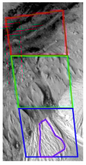
Figure 1.
Study area for photoclinometry on the flank of Aeolis Mons in Gale crater, Mars. A portion of HRSC nadir image h4234_0001, orthorectified based on the HRSC USGS stereo DTM at 50 m ground sample distance (GSD) is shown. The HiRISE reference DTM T1 covers the combined area outlined. Colors indicate subareas with different slope and albedo properties for which results appear in Figures 9 and 10. Local albedo variability decreases and surface roughness increases from red to purple. Equirectangular projection with north at top, latitude of true scale 0° N, 7 × 13.75 km, centered near −4.8° N, 137.8° E.
2.1.2. Jezero Crater
To support landing site selection, planning, and onboard navigation during landing for Mars 2020, the USGS produced DTMs from multiple HiRISE and CTX stereopairs, then coregistered them and made DTM mosaics as summarized below [12,13]. We used the mosaics rather than individual DTMs for this paper. The study area is defined by the HiRISE coverage, centered on the Jezero delta near latitude 18.49° N, longitude 77.41° E (Figure 2). These data cover approximately 290 km2 within a 20 × 20 km region, 5-fold the area studied at Gale. The HRSC product from DLR used in this study was a multi-orbit mosaic prepared for the Mars 2020 project. This DTM was not released, but readers wishing to replicate our work could utilize the Level 5 (multi-orbit DTM and orthoimage mosaic) product set [18] covering the half-quadrangle MC-13E including Jezero that has since been completed [19] and is available at http://hrscteam.dlr.de/HMC30/index.html (accessed 1 September 2021). The MC-13E DTM is based on the same images covering Jezero as the unreleased product, with additional images added to extend the spatial coverage. Level 2 images h5270_0000_xx2, available in the PDS, were used to produce single-orbit HRSC DTMs in SOCET SET and ASP. We also used CTX images J03_045994_1986_XN_18N282W and J03_046060_1986_XN_18N282W to produce DTMs in ASP. This is the same stereopair that provides coverage over the HiRISE DTM within the Mars 2020 CTX mosaic.
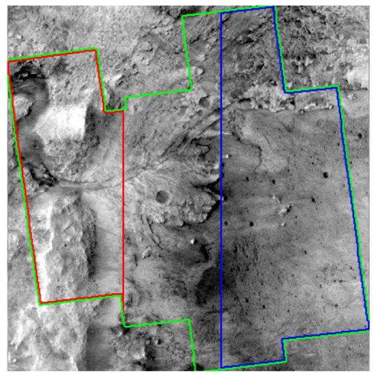
Figure 2.
HRSC orthoimage of study area in Jezero crater, Mars, derived from h5270_0000 nadir image at 50 m GSD. Area covered by HiRISE reference DTM mosaic (root mean squared slope 7.09°) is outlined in green, western rough (11.29°) subarea in red, and eastern smooth (3.38°) subarea in blue. Quality statistics for these areas are shown in Figure 6. Equirectangular projection with north at top, latitude of true scale 18.6° N. Area shown is 21.1 × 21.35 km, centered near 18.5° N, 77.4° E.
2.2. Mapping Methodologies
2.2.1. DLR HRSC Team Pipeline
The HRSC processing pipeline used at DLR is entirely automated and designed to take full advantage of the multi-line scanner geometry of the images. Products are controlled to MOLA by a sequential photogrammetric adjustment [20]. The Gale DTM is a Level 4 product, derived from a single-orbit image set [21]. Production of multi-orbit Level 5 products such as that used at Jezero is described in [18]. Dense image matching is described in detail in [21]. The images are filtered to reduce noise and compression artifacts, and orthorectified based on MOLA topography to reduce scale errors and parallax distortions. Area-based matching is applied, consisting of normalized cross correlation followed by subpixel refinement by adaptive least squares. Matching is performed at a “pyramid” of resolution levels because image quality usually varies within a single image strip (hundreds of kilometers long) for HRSC, depending on atmospheric and illumination conditions. Points from different resolution levels are filtered separately, then combined by weighted interpolation. This procedure improves matching performance in areas of poorer image quality and thus reduces the occurrence of matching gaps at the price of a small reduction in point precision in areas with higher image quality. Ground coordinates are computed by multi-ray intersection based on all available images, which provides information needed to eliminate bad matching results.
2.2.2. SOCET SET
Routine production of stereo DTMs at the USGS uses the same software for all image types. The open-source ISIS system developed by the USGS [22,23] is used for data preparation and commercial stereo software (SOCET SET® from BAE Systems [24,25]) is employed for control and DTM generation. Software providing an interface between these systems for planetary data is also available from the USGS [26]. BAE has since introduced SOCET GXP as the successor to SOCET SET. Our results can be expected to apply to future products made with SOCET GXP, because the adjustment and matching modules from SOCET SET are also used in GXP. ISIS was used to format output products for delivery, and for much of the analysis described below. We have described the mapping procedure for HiRISE in detail [27] and a tutorial is available online [26]; the procedure for CTX follows the same steps. We have also described the procedures for HRSC in detail [10,11]. These references also describe a more efficient approach to generating ground control that was applied to the Jezero HiRISE and CTX data. The differences in processing approaches, and the subsequent processing performed to refine and assess the geometric registration of the Jezero products [12,13] are relevant to the reliability of our DTM comparisons, so we summarize them here.
At Gale, HiRISE (and CTX) DTMs were produced from individual stereopairs over a period of several years. They were controlled by using the older procedure [27], in which ground control points were measured interactively. A small number of points in level areas were constrained in elevation, as interpolated from the MOLA data. An even smaller number of points on features common to the MOLA and image data were constrained in all three dimensions. Accuracy of the control was therefore limited by the sample spacing and GSD of MOLA. We investigated the consistency of the overlapping HiRISE DTMs and found offsets on the order of 100 m horizontally and 10 m vertically [9]. In addition, we discovered late in the process that geometric distortions in CTX images were not corrected properly, resulting in horizontal and vertical distortions of tens of meters. The CTX products were therefore adjusted horizontally to match the DLR HRSC data by “rubber sheet” transformation based on interactively measured ties, then the HiRISE products were warped to match CTX. This process left the horizontal accuracy of registration uncertain, but likely at the few-pixel level given the use of interactive measurements. Elevation differences were minimized by least-squares adjustment of vertical offsets to the DTMs, but mismatches of up to 10 m vertically remained as a result of uncorrected tilts [9]. These seams in the DTM mosaic led to the decision to restrict analysis to an area of the mosaic within the single T1 HiRISE DTM.
The USGS HRSC DTM was produced later [10] and controlled separately as outlined below. In that study, we found this DTM to be slightly misaligned with respect to the CTX and HiRISE products and shifted it to align it (by eye) with the HiRISE data. This process yielded single-pixel registration accuracy at best. The sparsity of small topographic features made it difficult to assess distortions that the warping process could have introduced into the reference DTM. Because Gale contains diverse albedo and slope features that are nearly ideal for testing the effects of sharpening DTMs with photoclinometry, for this study, we registered the undeformed HiRISE DTM from a single pair T1 to the USGS HRSC DTM by point-cloud fitting and rigid transformation with the ASP application pc_align.
The ASP point-cloud fitting module pc_align has also been used to generate dense sets of pseudo-ground control points for more recent DTMs including Jezero, by transforming a set of tiepoints with a rigid translation and rotation to align them with a topographic base. This process, described in [10,11], is significantly faster and more accurate than the earlier use of sparse manual ground points. MOLA altimetry or (where available) HRSC DTMs can be used as the base, but at Jezero a CTX DTM mosaic served this purpose [13]. Multiple overlapping CTX images were bundle-adjusted at JPL with custom software that corrected for spacecraft jitter as well as ensuring registration to the HRSC Level 5 product. The USGS then produced CTX DTMs in SOCET SET based on this control solution. The individual DTMs were then adjusted with pc_align by rigid translation only to minimize differences where they overlapped, and mosaicked. The mosaic was then translated to fit the Level 5 DTM. All HiRISE images were then controlled simultaneously with pseudo-ground control from the CTX mosaic and tiepoints between overlapping stereopairs. An initial comparison of the CTX and HiRISE mosaics revealed a small discrepancy in scale of ~0.3% in the cross-track direction, which was removed by an affine transformation of the HiRISE mosaic [13]. To further improve on the spatial accuracy achieved by bundle adjustment, Fergason et al. [12,13] used pc_align to fit the HiRISE DTMs to the CTX base. They then performed a cross-correlation analysis of the orthoimages associated with the transformed DTMs to verify that the spatially resolved offsets between DLR, CTX, and HiRISE products generated for Mars 2020 were small compared to the DTM GSD. Their correlation analysis revealed a small cross-track-scale discrepancy between the Level 5 HRSC DTM and the CTX (and adjusted HiRISE) DTMs, which they did not attempt to correct. The DLR DTM appears to agree more closely with the unscaled HiRISE DTM. Over the area covered by HiRISE scale error of 0.3% results in a root mean squared (RMS) registration error of ~17 m, or ~0.33 of an HRSC DTM post.
We controlled HRSC images used in the SOCET SET DTMs produced for this study to the Mars 2020 CTX mosaic by the procedure used for HiRISE in [12,13], and used pc_align to further improve the registration. The horizontal alignment accuracy between these products and the CTX mosaic was estimated as part of the DTM comparison process as described below. The two-dimensional alignment error was found to be 18 m. Thus, all datasets are aligned horizontally with fractional-post precision. In preparing the products for this study, we discovered that an east–west tilt of ~0.09° exists between the Level 5 DTM and the other products. Given that the Level 5 product was controlled to MOLA over a broader area, it is probably correct and the Mars 2020 products are tilted. We nevertheless adjusted the tilt of the Level 5 DTM to agree with the other products for purposes of this study. The mean vertical offsets between DTMs are unimportant because we focus on the dispersion in elevation differences.
Stereo matching in SOCET SET was performed by using the Next-Generation Automatic Terrain Extraction (NGATE) module [28,29]. NGATE uses both area- and feature-based matching to estimate heights “at every pixel” (i.e., on a grid with GSD equal to the mean GSD of the input images). Estimates can also be based on more than 2 images, but these are considered pairwise (including both orderings of each pair) rather than in a multi-ray intersection calculation. The dense height estimates from multiple pairs and algorithms are then combined to generate an output at the desired GSD by a proprietary process that incorporates blunder detection and consistency checking. Four levels of additional smoothing of this output (none, low, medium, and high) may be selected. Unsmoothed NGATE DTMs from Mars images tend to have a “blocky” appearance (Figure 18 in [27]) that causes RMS surface slopes to be overestimated. Rather than using the smoothing options built into NGATE, our standard procedure for multiple mapping projects as well as previous DTM quality assessments has been to apply a single pass of the older, area-based Adaptive Automatic Terrain Extraction (AATE) algorithm [30] to the NGATE result to reduce the appearance of blocky artifacts. Our rationale for using AATE is that smoothing as a side effect of area-based matching might be expected to introduce fewer errors than a filter that does not consider the image content. We refer to DTMs produced by using this standard NGATE+AATE procedure as “USGS DTMs,” consistent with our earlier usage [9,10,11,14] when the only USGS-produced DTMs analyzed were made in this way. In this paper, we make a quantitative assessment of the results of the NGATE+AATE procedure and compare it to DTMs using each of the levels of NGATE smoothing and to unsmoothed NGATE DTM that were post-processed using lowpass boxcar filters of various sizes. SOCET SET provides tools for interactive editing, but no editing was performed on the DTMs used in this study.
2.2.3. Ames Stereo Pipeline
HRSC and CTX image data were prepared for processing in ASP closely following the procedure described for CTX images in [31]. The images in each stereopair were first controlled relative to one another using the ASP bundle_adjust tool, which automatically establishes tiepoints between the images. ASP was next used to collect an initial point cloud, which was fitted to the USGS CTX DTM mosaic reference using ASP’s pc_align tool. The initial point cloud was also used to create a sparse preliminary DTM. The input images were then orthorectified onto this sparse DTM in preparation for subsequent rounds of dense matching using the various stereo parameterizations in ASP described below. ASP provides the capability to do multi-image matching (>2 images) and multi-ray intersection. This capability was used to produce the majority of the HRSC DTMs studied from the triplet of stereo and nadir channels. For some matcher parameters, DTMs were also produced from the pair of stereo channels alone. The registration of completed DTMs to the Mars 2020 CTX mosaic was refined by using pc_align. The CTX DTMs made by this process were clearly affected by jitter, which was corrected for in the control process used for the Mars 2020 CTX mosaic but not by the independent control process in ASP. Within Jezero crater, the ASP CTX DTMs were offset horizontally by approximately 1 post (20 m) north–south from the HiRISE DTM mosaic; although the use of pc_align removed the mean shift over the full overlap area between our DTMs and the CTX base, jitter distortion resulted in residual errors locally. We corrected this local offset to the nearest whole post as determined by visual examination of the difference between reference and (shifted) target DTMs. The elevations also contained “ripple” artifacts (high and low bars extending across track; cf. [32]) that are absent from the mosaic. To minimize the impact of these artifacts on our quality statistics, we excluded from consideration the areas at the northwest and southeast corners of the HiRISE coverage that were most affected.
The default stereo matching process in ASP is “block matching,” which consists of normalized cross correlation (NCC) followed by subpixel (SP) refinement by one of several algorithms available in ASP [33]. We investigated the quality of DTMs produced without SP refinement, with refinement by parabolic interpolation of the NCC results, and by Bayesian expectation maximization weighted affine adaptive window correlation (“Bayes EM”). We did not test the simpler, nonadaptive affine SP algorithm that is also offered. The kernel sizes for the NCC and affine SP steps are the parameters most obviously related to DTM resolution. We therefore investigated combinations of odd NCC kernel sizes from 3 to 25 pixels and odd SP sizes from 7 to 25 pixels.
ASP also includes several matchers based on Semi-Global Matching (SGM) [34], which attempts to find a distribution of stereo disparities that is consistent with correlation results. By optimizing a robust cost function, SGM attempts to interpolate smoothly where the correlations are noisy (e.g., featureless areas), yet allows sharp jumps in disparity where justified by the data. The method thus offers the hope of better performance on both bland and steep terrains. SGM has been applied successfully to HRSC images [35] and was evaluated in the HRSC DTM comparison [1]. ASP offers both a generalization of the original SGM algorithm and More Global Matching (MGM) [36], also known as smooth SGM. We tested both algorithms over the kernel sizes supported by ASP (odd, 3–9 pixels). We also compared results with and without SP refinement (which is built into SGM and MGM and does not require specifying a separate kernel size) and with two different cost functions that control how large and small parallax changes between neighboring pixels are weighted in creating the DTM. Cost mode 3 uses the census transform [37] and cost mode 4 uses the ternary census transform [38]. The latter is expected to be more stable on low contrast terrain but may be less accurate elsewhere [33].
2.2.4. Photoclinometry
To investigate the effects of refining a stereo DTM by photoclinometry, we used the ISIS 2 software and methods described in [39] to process a subarea of the HRSC nadir orthoimage circumscribing the HiRISE T1 DTM (Figure 3). This software can be used to process geometrically raw images (yielding a shape model in camera coordinates that must be map projected). Processing an orthoimage is preferable, however, because the coregistered stereo DTM is helpful or essential at several steps in the procedure. The photoclinometry algorithm takes a single image as input and necessarily assumes that the surface albedo is uniform, which is obviously not true for most of Mars. The T1 area, in particular, contains terrains ranging from a dune field in the north with low slopes and extreme albedo variations to the rugged slopes of Aeolis Mons with more subtle albedo variations in the south. We therefore utilized the HRSC stereo DTM to estimate and subtract the contribution of atmospheric haze to the image and then to correct for albedo variations down to its limit of resolution. The steps of this process [40] are illustrated in Figure 3. First, a synthetic image is computed from the DTM (Figure 3b), based on the illumination and viewing directions for the real image and a realistic photometric function appropriate to the phase angle [39]. Neglecting resolution effects for the moment, the true image is approximately this synthetic image times the spatially varying albedo, plus the atmospheric contribution. The intercept of a pixel-by-pixel linear regression of the observed brightness on the model therefore yields an estimate of the haze brightness. In the present case, this intercept was close to the intensity of the darkest pixels in the study area, indicating the dark pixels were likely shadows and further confirming the haze estimate [39]. Figure 3c shows the ratio of the true image (with haze subtracted) to the model. Resolution aside, this should be a map of relative albedo. In reality, it contains contributions from both topographic and albedo features smaller than the resolution of the stereo DTM. We therefore smooth this ratio at the DTM resolution (which is known from the results above) to obtain a smooth albedo map (Figure 3d). Dividing the (haze-subtracted) image by this albedo estimate yields a product (Figure 3e) that contains topographic shading at all length scales, but only the albedo features smaller than the stereo DTM resolution. The severity of these uncorrected albedo variations varies greatly; in the north, they appear more prominently than the real topography (as shown by the HiRISE reference DTM in Figure 3g), but in the southernmost part of the area, they are almost unnoticeable. The corrected image was used as the input to the photoclinometry algorithm, and the stereo DTM was used as the initial approximation to the topography. We solved the photoclinometry equations iteratively by under-relaxation, with relinearization after every relaxation step [39]. The result was saved and evaluated after 1, 2, 4, … 128 steps. Note that for this test we generated the orthoimage at the DTM GSD. It would also be possible to prepare the orthoimage at a higher resolution (in particular, matching the GSD of the raw image), in which case it would be necessary to interpolate the stereo DTM to match. We will discuss the pros and cons of using a full-resolution orthoimage below.
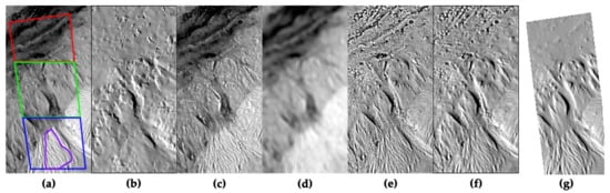
Figure 3.
Processing of HRSC data overlapping the HiRISE Traverse 1 (T1) stereopair in Gale crater, Mars to correct albedo variations in HRSC image and refine stereo DTM by photoclinometry. (a) Portion of HRSC orthoimage of h4234_0001 nadir image at 50 m GSD, also shown in Figure 1. Quality statistics for areas outlined in color are shown in Figures 9 and 10. (b) Synthetic image from USGS HRSC stereo DTM. (c) Ratio of orthoimage (after haze subtraction) to synthetic image contains albedo variations and shading due to topography not resolved in stereo DTM. (d) Ratio c, smoothed at the DTM resolution of 7 posts, contains albedo variations over larger distances than this. (e) Ratio of orthoimage a (haze subtracted) to smooth albedo d contains shading plus albedo variations smaller than 7 pixel resolution. This image was used as input to photoclinometry to refine the stereo DTM. (f) Synthetic image from stereo DTM refined by photoclinometry after 16 iterations. (g) Synthetic image from HiRISE T1 DTM downsampled to 50 m GSD. Photoclinometry result f appears similar except where image e contained uncorrected albedo variations. All panels are in Equirectangular projection with north at top, latitude of true scale 0° N, 7 × 13.75 km, centered near −4.8° N, 137.8° E.
2.2.5. Quality Assessment
Our primary approach to quality assessment is the comparison of target DTMs to reference DTMs with significantly (by a factor of 20 or more in the cases shown, though a smaller ratio would likely suffice) better resolution and vertical precision. This process, which is illustrated in Figure 4, begins with downsampling a HiRISE reference DTM (or DTM mosaic) from its original GSD of 1 m/post to the appropriate GSD and reprojecting it to match the “target” DTM to be evaluated. In the latter step, not only the projection type, but scale, extent, and any projection parameters such as the latitude of true scale must be matched exactly. We then smooth the reference DTM with boxcar lowpass filters of 3 × 3, 5 × 5, etc., posts, and measure the RMS difference between the target DTM and each of these smoothed products. As discussed in Section 4, in order to obtain the most precise results, the smoothed reference DTM should be trimmed to eliminate edge effects near the boundaries of the valid data. This step was omitted in our analysis of Jezero DTMs, but the lowpass filter was not allowed to extrapolate beyond the edge of the reference data, which would lead to even greater errors. We estimate based on limited tests with and without trimming that our untrimmed results systematically understate the resolution of HRSC DTMs by ~10% or less and of CTX DTMs by ~3% but that the effect on vertical error estimates is negligible. Edge effects will be larger for smaller DTM areas or rougher terrains, so the trimming step should be incorporated in any future studies. Strictly speaking, we tabulate the standard deviation of the difference, which is equivalent to calculating the RMS difference after making a small vertical adjustment to eliminate the mean difference between DTMs in each pair being compared. Inverse quadratic interpolation of the difference at odd-integer filter sizes then yields the filter size at which HiRISE best fit the other dataset (a measure of resolution) and the minimum difference (a measure of vertical precision). In order to compare results from HRSC and CTX (and extrapolate to other imagers) it is useful to normalize these quality factors. The best-fit filter size can be expressed in pixels (i.e., the value in DTM posts is multiplied by the DTM GSD and divided by that of the images). If we assume that local image matching error is the main contributor to vertical errors, we can equate the RMS elevation difference at best fit to the expected vertical precision EP of the DTM. Note that this is not always an accurate assumption; internal distortions in the target DTM (e.g., from spacecraft jitter) or the reference DTM (from residual errors in aligning multiple stereopairs) can also contribute to the difference, increasing the apparent vertical and matching errors.
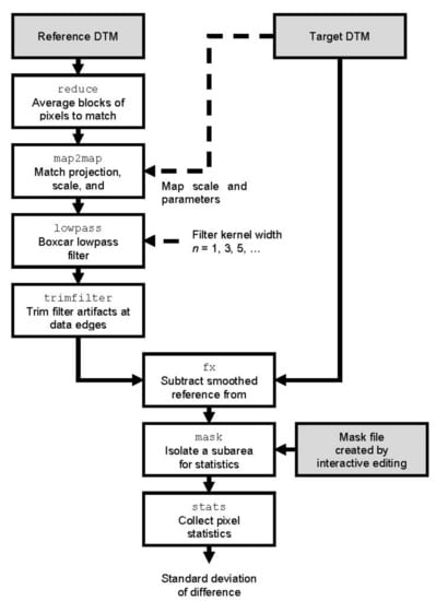
Figure 4.
Flowchart showing the processing steps used to compute the RMS difference between a target DTM and a (smoothed) reference DTM. Names of the ISIS programs used for each step are shown in monospaced font. The three lowest values of the standard deviation of difference as a function of filter kernel width n are interpolated to estimate the vertical precision EP of the target DTM as the minimum difference, and the horizontal resolution as the interpolated filter size at which the minimum occurs.
The expected vertical precision can then be related to the RMS matching error ρ in pixels by the equation
where p/h is the parallax to height ratio of the stereopair and GSD is the ground sample distance of the images, not that of the DTM. Reference [41] gives a vector formula for p/h that is valid for any viewing geometry. For HiRISE and CTX pairs, and on the midline of HRSC imager swaths, the look directions for the paired images line in a plane. In this restricted geometry, p/h approximately equals the sum of tangents of the two emission angles (or the difference of the tangents if both images are taken from the same side of the target point, as in some HiRISE and CTX pairs). At the edges of an HRSC swath, p/h will be slightly greater than on the midline because the finite field of view contributes to the parallax. Note that the channels of an HRSC image set are often recorded at different ground sample distances by averaging different sized blocks of pixels. This introduces the question of how to normalize errors for a DTM made from images with significantly different GSD. As we show below, we obtain consistent results between CTX and HRSC by normalizing to the GSD of the stereo channels, which is typically twice as large as that of the nadir image.
EP = ρ GSD/(p/h)
For brevity, we refer to these quality factors, whether in meters or normalized to pixels, as “resolution” and “error” (or “precision”) below. We compare our estimates of DTM resolution and precision by comparison to a reference DTM with other quantitative and qualitative estimates. Calculating topographic slopes as a function of baseline can provide information about resolution and artifacts. Elevation errors can sometimes be assessed without a reference DTM by looking at the dispersion of height values in flat areas. Visual examination of the DTMs can yield information about the spatial characteristics of errors. Comparison of shaded reliefs computed from the DTMs to the corresponding orthoimages is especially helpful. Assessing the smallest real features that are reliably seen gives a measure of resolution [1].
3. Results
3.1. Comparing Reference and Target DTMs
Results for the DLR Level 5 HRSC DTM and USGS (SOCET NGATE + AATE) HRSC and CTX DTMs are shown in Table 1 and Figure 5. Figure 5a shows the results in meters for each discrete filter size used. In Figure 5b, the normalized results are shown, and only the smooth curve through the data and the interpolated optimum are plotted for each DTM. The HRSC stereo channel GSD has been used in the normalization; this yields better consistency between the cameras than using the nadir GSD, which is a factor of 2 smaller. Normalization by the stereo channel GSD is reasonable given that these channels contribute the most parallax to the stereo set. Results (both precision and resolution) for the same camera and processing are consistent at approximately the 15% level between sites. The HRSC USGS products have significantly larger errors than the DLR DTMs. They also have better (smaller) resolution (i.e., the minimum error occurs at a smaller filter size for the USGS DTMs). The normalized CTX results plot closer to those for the DLR DTMs (better precision and poorer resolution) despite the DTM being generated with the same software as the HRSC USGS DTMs. Already with the five best-fit points shown in Figure 5b, there is a suggestion of a negative trend between resolution and error.

Table 1.
DTM resolution and error based on comparison to smoothed HiRISE data.
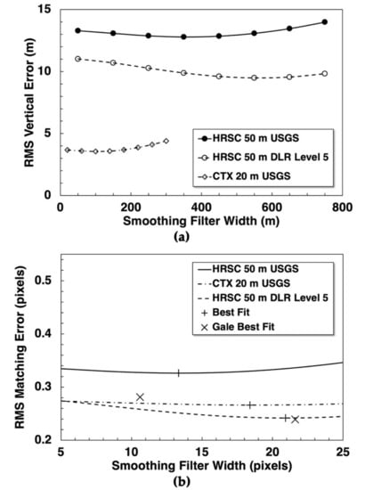
Figure 5.
Estimated matching error of target DTMs as a function of smoothing of reference DTM. (a) Filter width and RMS vertical difference in meters. Values for odd-integer filter widths are shown, connected by a smooth curve. (b) Filter width and error nondimensionalized in terms of stereo channel GSD and stereo parallax/height ratio as described in text. Curves through data are shown with crosses indicating the interpolated minimum error at best-fit width. Xs indicate interpolated minima for Gale crater results [10,11] with DLR point to right of that for USGS DTM.
An important question is whether these results are predictive of the quality of other DTMs made with images from the same camera and analyzed with the same software, or whether they are somewhat specific to the terrains studied. The consistency between the Gale and Jezero results supports the former expectation, but the diversity of terrains within the Jezero study area provides an opportunity to test it. We therefore analyzed subareas smoother and rougher than the average (Table 2). The smooth region (east of 77.45° longitude) lies entirely on the Jezero crater floor east of the delta. The rough region (west of 77.35°) consists primarily of the crater rim. Table 2 gives the RMS adirectional slope for these areas and the full HiRISE DTM, along with the normalized resolution and matching error. Note that the RMS slope values are greater at the 20 m baseline between posts of the CTX DTM than at the 50 m baseline appropriate to HRSC. Results for the DLR Level 5 DTM are nearly independent of terrain. Matching errors increase with roughness for the DTMs produced in SOCET SET, but much less than proportionately; the logarithmic derivatives (Table 2) are less than 0.5. The resolution increases with increasing terrain slope (again, much less than proportionately) for HRSC but not for CTX. The product of resolution and error is nearly independent of slope for both HRSC DTMs, but for the CTX data the resolution is nearly constant and both the error and the product increase with slope.
Table 2.
DTM normalized resolution and error as a function of surface slope.
We next consider the effects of different methods and degrees of smoothing the SOCET NGATE DTMs, including the behavior for smooth and rough subareas as well as the full DTMs. Figure 6a shows the matching errors for Jezero DTMs plotted as a function of resolution. The points for “NGATE Smoothing” correspond to the NGATE settings of none, low, medium, and high. Results for the basic NGATE result (no smoothing in the matcher) smoothed by an odd-sized boxcar lowpass filter in ISIS are labeled “LPF Boxcar.” In both cases, the amount of smoothing applied increases toward the lower right. The “+AATE” points reflect the standard USGS processing and are the same as in Figure 5. The most obvious results are that, for a given area, the different methods of smoothing the basic NGATE DTM follow nearly the same approximately inverse trend, and that areas of differing roughness follow similar but offset trends. As noted above, the DLR DTM shows much less variation in error and almost none in resolution as a function of terrain. It is plausible that the error and resolution of the basic NGATE result vary with slope as a result of the nonlinear process by which height estimates “at every pixel” are combined to yield the output DTM. Figure 6 shows that the unsmoothed NGATE product exhibits slope-dependent resolution and error very similar to the pattern seen in the AATE-smoothed USGS product in Table 2. The approximately inverse relation between resolution and error after further smoothing of the NGATE DTM in a given region is not surprising. For linear averaging of independent height samples (e.g., by a smoothing filter larger than the size of any correlated errors), one would expect the RMS error to vary inversely with filter width so that their product is constant. Figure 6b shows that the product of resolution and error for smoothed NGATE DTMs is approximately constant but displays a weak minimum whose value is almost independent of slope. This minimum occurs near the NGATE+AATE (USGS) and 5x5 boxcar results and between the low and medium smoothing options. The NGATE+AATE approach that the USGS has used extensively is thus close to a loosely defined “sweet spot” in terms of overall DTM quality. Somewhat disappointingly, post processing with a simple 5x5 lowpass filter yields better resolution at a similar error level to AATE despite not taking the images into account and is undoubtedly faster to compute. Compared to these products, the DLR Level 5 DTM is significantly smoother, but its product of error and resolution is similar. Smoothing the NGATE DTM with an 11x11 boxcar filter results in quality statistics very similar to the DLR product, though slightly more terrain dependent.
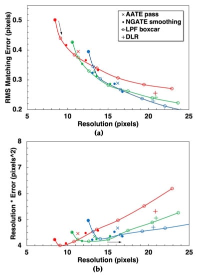
Figure 6.
Normalized resolution and error for Jezero HRSC DTMs. (a) Results from commercial SOCET SET/GXP matcher NGATE. Large solid circles represent the basic NGATE output. Other symbols show the effects of various smoothing approaches (see text for full description) plus DLR Level 5 product, as listed in key. (b) As (a) but showing the product of resolution and error. In both panels, red, green, and blue colors correspond to rough, full, and smooth areas outlined in Figure 2. Arrows indicate direction of increasing applied smoothing.
Estimating slopes over small horizontal baselines is an important application of planetary DTMs and is crucial for landing site selection and validation. We therefore calculated the RMS adirectional slope on a one-post (50 m) baseline for the suite of SOCET SET HRSC DTMs and compared the results to slopes computed from the reference DTM (Figure 7). ISIS program deriv was used to compute first differences in the row and column directions. These were converted to bidirectional slopes in degrees by using fx, which performs general pixel algebra. RMS adirectional slopes were then computed by taking the root summed square of the two bidirectional slopes. Regardless of terrain, the “blocky” NGATE DTM substantially overestimates the RMS slope as a result of its large vertical errors. Smoothing the DTM decreases the slope estimates, bringing them into better agreement with the true slopes. No single smoothing solution yields consistent agreement with the more accurate, HiRISE-derived slopes for all three study areas; this is unsurprising given the terrain-dependent behavior built into NGATE. The curves for increasing DTM smoothing on each terrain each exhibit a “knee” close to the 5 × 5 lowpass filter point. Up to this filter size, increasing smoothing mainly decreases slope errors with relatively little degradation in resolution, whereas for larger filters the slope error decreases less for given loss of resolution. The 5 × 5 lowpass filter also arguably comes close to being optimal in terms of consistency. It overestimates slopes of 7° and 11° by 0.8° and 0.6°, and the 3.4° slope of the Mars 2020 landing area by 2°. The USGS (NGATE+AATE) approach does a little worse but is also fairly consistent, with errors ranging from 1.3° to 2.2°. In a relative sense, the slope errors for the smooth terrain are substantial, but errors of one or two degrees will not affect the ability to distinguish safe from hazardous landing sites. Maximum acceptable slopes at short baselines are much greater, ranging from 15° [42] to 30° [8]. Overestimating slope hazards slightly is clearly preferable to underestimating them in this application. The variation of slopes (and slope errors) with baseline is described below.
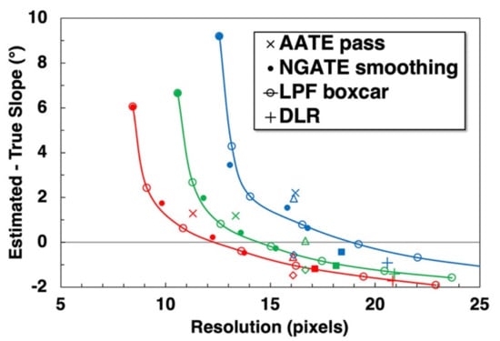
Figure 7.
Error in RMS adirectional slope at 50 m baseline computed from various HRSC DTMs, compared to slope estimated from HiRISE data. Symbols indicate DLR Level 5 and various smoothed SOCET NGATE DTMs as in Figure 6. Results for ASP DTMs are also shown, with symbols as in Figure 8. Red, green, and blue colors correspond to rough, full, and smooth areas outlined in Figure 2.
Results for DTMs produced with the ASP block matcher are shown in Figure 8a, with the NGATE and DLR results from Figure 6b for comparison. The models differ mainly in error. Resolutions range only between 17 and 20 pixels rather than tracking the kernel size as the smoothed NGATE models do with filter size. Not surprisingly, subpixel interpolation reduces errors compared to the NCC result with no refinement, but results from the adaptive affine algorithm are better yet. Visual inspection shows that the larger errors in the models with interpolated or no SP refinement mostly take the form of local “blunders” (small patches with much larger residuals than typical). The abundance and typical size of such blunders decrease as the NCC kernel size is increased. Contouring artifacts were not observed, though they might be expected not only for whole-pixel matching as a result of quantizing the parallax but also for interpolated subpixel correction as a result of pixel-locking [43]. If the affine subpixel refinement is not used, increasing the NCC kernel size reduces the error up to a point, after which it tends to increase (worsen) resolution slightly with little effect on the product. Varying the affine SP kernel size for fixed NCC kernel yields a similar “L-shaped” curve. The best resolution occurs at a SP kernel size of 13 pixels and has an error that decreases only slightly with increasing NCC kernel size, converging for NCC kernels approaching 25 pixels. It thus appears that SP refinement produces the same results as long as elevations computed in the NCC step are sufficiently close to correct. Note that the best block matcher result falls directly on the curve for lowpass filtered NGATE models, close to the 9 × 9 filter result. Resolution and error vary only slightly with terrain roughness, as shown in Figure 8a for the best model (results for the other algorithm and parameter choices show similar variation but are omitted for clarity). Slopes computed from the best block matching DTM underestimated the true values on all terrains by amounts ranging from 0.4° to 1.2° (Figure 7).
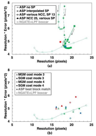
Figure 8.
Quality factors for Jezero HRSC DTMs produced by using the Ames Stereo Pipeline. The product of resolution and matching error is plotted as in Figure 6b. Colors correspond to areas of different roughness outlined in Figure 2. (a) Results for block matching. Arrows indicate direction of increasing kernel size. For NCC with no subpixel refinement (open diamonds) or parabolic interpolation (diamonds), the product of resolution and error first decreases at constant resolution as NCC kernel size is increased, then remains almost constant as resolution increases slightly. With adaptive affine subpixel refinement, increasing SP kernel size at fixed NCC kernel size yields similar behavior (squares), but increasing NCC kernel size (open squares) has little effect. For clarity, results for rough (red) and smooth (blue) subareas are plotted only for the optimum set of kernel sizes. (b) Results for the ASP SGM and MGM matchers with two cost functions (see text). Results are shown for a kernel size of 9 pixels, which yielded the best DTM quality.
Results for the ASP SGM and MGM algorithms are shown in Figure 8b. The NGATE, DLR, and best ASP block matcher results are included for comparison. DTMs produced without subpixel refinement and those made with kernel size 3 are not shown because their errors were much larger. For clarity, results for the smooth and rough terrains are shown only at kernel size 9, which produced the best product of resolution and error in each case. As expected, the ternary census transform (cost mode 4) produces better results on smooth terrain but worse results on rougher terrain, whereas the terrain dependence with mode 3 is weak. Resolution is nearly independent of terrain roughness for each combination of algorithm and cost model. The average resolution and error for mode 4 are similar to those for the DLR pipeline. MGM yields slightly better resolution but similar resolution-error product than SGM, hence larger errors. The visual appearance of the SGM models is also smoother, which is opposite to what is described in [33]. Contouring artifacts, which were present in parts of the SGM models in [1] were not observed. “Cloth-like” textures, with artifacts along the cardinal and diagonal directions, were present in the DTMs made with smaller kernels but subtle or absent from the best models made with a 9 pixel kernel. The MGM algorithm with cost mode 3 overestimated slopes on smooth terrain by 2° and yielded the correct average for the full study area, but slope estimates for all other combinations of algorithm and region were underestimated by amounts ranging from 0.6° to 1.5° (Figure 7).
All of the HRSC DTMs described so far were derived from the triplet consisting of the two stereo channels, which have 26.9 m GSD, and the nadir channel, with pixels a factor of 2 smaller. To assess the contribution of the nadir channel, we made and evaluated Jezero DTMs from the stereo channels alone with SOCET SET and the ASP block matcher. The kernel sizes used for the block matcher were those found optimal for the image triplet above (25 pixels for NCC and 13 for SP). The results are summarized in Table 3. Fractional improvements for unsmoothed NGATE were similar to those for the USGS combination of NGATE+AATE, so are not shown. For NGATE+AATE, the estimated resolution for the triplet is approximately 80% that for the pair, which corresponds to the change in the dense grid spacing used by NGATE, given that this equals the mean of the input image GSDs, and the GSD of the nadir channel is half that of the stereo channels. Introducing the nadir image reduces (improves) the error level to approximately 75% of that for the pair. This is less than the improvement that would be expected if the three pairs formed (nadir-stereo 1, nadir-stereo 2, and stereo 1-stereo 2) were statistically independent, but it clearly represents a simultaneous improvement in resolution and error, rather than the trade between the two that smoothing the DTM provides. In stark contrast, the ASP block matcher gave almost identical results with and without the nadir image. The default behavior of ASP, reflected in this test, is to match images that have all been orthorectified at the coarsest GSD of any image in the set. This results in undersampling of the nadir image in the HRSC triplet, so we produced additional DTMs based on both the triplet and stereo–stereo pair orthorectified at 13 m/pixel. We varied the kernel sizes to find the optimum settings appropriate to the smaller orthoimage GSD. The optimal SP kernel size was again 13 pixels (in a few cases, the resolution at 11 pixels was best, but that for 13 pixels was extremely similar in all these instances). The frequency of blunders and gaps decreased more gradually as the NCC kernel was expanded than with the 27 m orthoimages. As the kernel size approached 49 pixels (approximately twice the value required for the undersampled images) the error became nearly constant, though a few blunders remained. As shown in Table 3, adding the nadir image improved resolution and error slightly more than when it was undersampled, but the improvement was still much less than in SOCET SET. A striking difference (which is not reflected in the table) is that the point cloud contained a larger number of small “holes” that had to be filled by interpolation when the nadir image was omitted. It should also be noted that, compared to the default orthorectification, using 13 m/pixel orthoimages decreased (improved) DTM resolution by approximately 15% but increased the match error and the product of resolution and error significantly.
Table 3.
Effect of adding HRSC nadir image to pair of stereo channels.
We also used the ASP block matcher to produce DTMs from a CTX stereopair with various combinations of kernel sizes. Our goal was not to compare the resolution and precision of the best result to the quality of the CTX DTM mosaic made in SOCET SET, because the single pair was less precisely registered and we analyzed a smaller area to avoid the worst jitter artifacts. Instead, we compared the variation in relative quality as the kernel sizes were varied and the optimal kernel dimensions with our results for HRSC. For CTX as for HRSC, the optimal SP kernel size was 13 pixels (or in a few cases 11 pixels with 13 an almost undistinguishable second best) regardless of the NCC kernel size. The matching error (and the abundance of blunders after the NCC step) declined in a few discrete steps as the NCC kernel size was increased. As in the case of HRSC, the total decrease in error with NCC kernel size was small, only ~15%. We speculate that these jumps in RMS error and accompanying changes in the locations of blunders may be triggered by changes in the way ASP tiles the images to parallelize matching as a function of kernel size.
3.2. Photoclinometry
The results of refining the HRSC USGS DTM by photoclinometry are shown in Figure 9. The RMS error is shown in meters; because the resulting DTM is no longer the product of stereo matching, we do not convert this to an equivalent matching error in pixels as we did in Figure 6a. The resolution is expressed in pixels of the image, in whatever form (raw or resampled) it was used in the calculation. Because we utilized an orthoimage matched to the stereo DTM, this pixel spacing is equal to the DTM GSD of 50 m/post. In interpreting these results it is helpful to understand that the iterative relaxation process adjusts slopes across one pixel at a time, so slopes on an N-pixel baseline are only beginning to adjust after N iteration steps and generally require several times N steps to converge. Because the goal is to refine details smaller than the stereo DTM resolution (~7 posts), a few times 7 iterations are likely to be needed, and this is observed in the figure. The resolution-error behavior can be divided into three phases. In the first few iterations, the error decreases and the resolution generally increases, similar to the effect of DTM smoothing seen in Figure 6a. This phase represents the rapid relaxation of localized artifacts created by the stereo matcher. In the second phase, resolution decreases (improves), but after 16-32 iterations (i.e., approximately 2–4-fold the initial resolution) the third phase is reached, during which the resolution remains nearly constant. Whether the error level decreases, stays the same, or increases during the second and third phases depends on the severity of uncorrected albedo variations. Figure 9a compares the behavior averaged over the whole test area for refinement based on the real image with that for a synthetic image calculated from the reference DTM. When the synthetic image, which includes no albedo variations and perfectly matches the assumed photometric behavior, is used, the error decreases in phase 2 and continues to decrease slowly in phase 3 when the resolution has reached its minimum. This minimum is ~2.5 posts rather than 1 post because computing the synthetic image requires interpolating and thus smoothing the reference DTM data. When the real image is used, errors increase slightly in phase 2 and more dramatically in phase 3. Figure 9b shows how the error is affected by albedo variations in real data. In the northern part of the study area, where relief is subtle and albedo variations are pronounced even after correction, the DTM error increases in both phases 2 and 3. In the central and southern thirds, the terrain becomes rougher and residual albedo variations less prominent. In these areas, the error remains constant as resolution improves, then increases in the final phase. When the statistics are limited to a small, rugged region with nearly uniform albedo, the behavior is similar but the resolution decreases even more, to nearly the level seen with synthetic data. Even for this subarea, however, the error increases in phase 3. The likely explanation is that even small albedo fluctuations (or even noise in the image) cause stripes (troughs and ridges in the direction of illumination) to form [32,39]. These artifacts “grow” away from their starting points at albedo fluctuations as iteration proceeds and thus introduce errors to an increasing fraction of the DTM. Figure 10 shows the evolution of the product of resolution and error as iteration proceeds. In addition to illustrating how the achievable improvement depends on the severity of albedo variations, the figure shows that near-optimal results persist over a broad range of iterations. The exact stopping point is not critical but should be in the range of 16-32 iterations for this DTM (the transition from phase 2 to phase 3 in Figure 9), or more generally 2–4-fold the resolution in pixels. The curve for synthetic data declines monotonically over the range examined, suggesting that increasing the number of iterations (as a multiple of resolution) may be useful in cases where the albedo is extremely uniform.
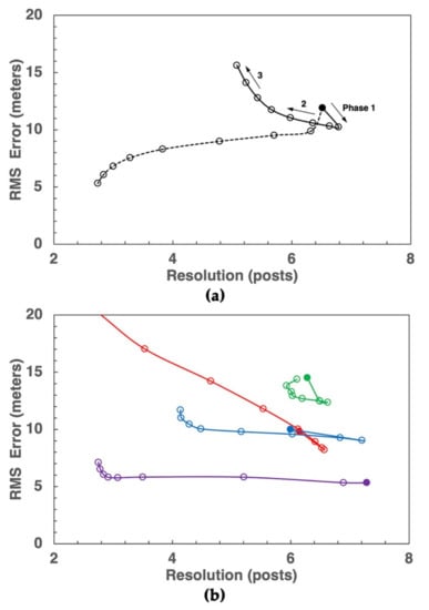
Figure 9.
Quality factors for Gale HRSC DTMs refined by photoclinometry. Note that the normalization to image GSD (appropriate to stereo and used in Figure 6a) is not used here. Best-fit filter width (resolution) is normalized to the DTM and orthoimage GSD and vertical error is in meters as measured. Solid circles show values for starting stereo DTM; open circles show results after 1, 2, 4, … 128 iterations. (a) Results for full area covered by the HiRISE T1 DTM. Solid line is for actual image data with albedo variations corrected based on stereo DTM, dashed line is for a synthetic image with uniform albedo computed from the reference DTM. (b) Results for iteration with the real image for subareas of differing slope and albedo variation outlined in Figure 3a. Three phases of changing resolution and error as iteration proceeds (arrows) are labeled for the full area but are identifiable in the other curves. See text for discussion.
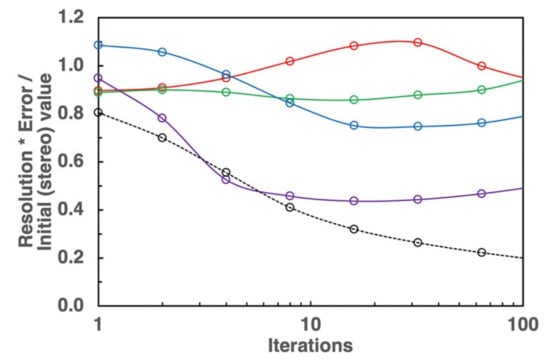
Figure 10.
The product of resolution and error, normalized to its initial value for the stereo DTM, versus number of photoclinometry iteration steps. Colors correspond to subareas in Figure 3a; black curve is for synthetic data with no albedo variation over the entire DTM.
If a GSD smaller than that of the stereo DTM is selected for photoclinometry, more iterations will be required to achieve optimal convergence, and each iteration will also take longer because of the larger number of pixels to be processed. The overall computational effort scales as the inverse cube of the GSD selected. Reducing the orthoimage GSD provides a possibility of resolving smaller topographic features in the final DTM, but it can also introduce smaller, uncorrected albedo variations that will create additional artifacts. Thus, whether it is worthwhile to use a full-resolution orthoimage and try to improve the DTM resolution to a fraction of the stereo DTM post spacing is a decision that depends critically on an evaluation of the smallest relief and albedo features that are visible in the image.
Figure 11 illustrates good and bad outcomes of refining the DTM by photoclinometry. Profile A-A’ is located in the southern part of the DTM where albedo variations are subtle to begin with and are diffuse enough to be corrected well (cf. Figure 3). The profile shows that the ridges and grooves have not only been added to the DTM in the correct locations, their amplitudes match the HiRISE reference data closely and the broader-scale slopes are well preserved. In contrast, profile B-B’ crosses a channel in the middle of the DTM where albedo is more variable. The albedo-corrected image (top center) appears to show a bright linear feature on the channel floor that is not present in the HiRISE shaded relief at right. In the original image (left) it is clearer this is an alignment of bright streak on the channel floor rather than a slope feature. The photoclinometry algorithm necessarily interprets the feature as topography, however, and adds a bench within the channel that may be geologically possible but is not supported by the image.
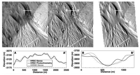
Figure 11.
DTM profiles across features without (A-A’) and with (B-B’) uncorrected albedo artifacts. Profile locations are shown on (left to right) HRSC orthoimage, HRSC image after correcting for albedo variations resolved by stereo DTM, and HiRISE shaded relief (cf. Figure 3a,e,g).
3.3. Slopes as a Function of Baseline
A fundamentally different approach to quantifying DTM resolution is to plot the RMS slope against the horizontal baseline over which it is evaluated. Slopes at every baseline value can be calculated efficiently by using fast Fourier transform methods, and such baseline-slope curves have been an important tool in landing site selection for numerous missions (e.g., [8,27]). Although the software used to generate these slope-baseline curves is unreleased, the equivalent information can be collected by using ISIS or other widely available software to calculate bidirectional slopes at one baseline at a time. As shown in Figure 12a, the slope curves can contain information about the data collection process as well as the surface topography. This approach addresses a wide range of spatial scales and does not require a reference DTM; resolution can often be inferred from a break in the derivative of the baseline-slope curve. A reference is nonetheless useful as an indication of the true surface slope behavior, so that only deviations from this are interpreted as data effects. The main drawback of using baseline-slope curves is that the results can be ambiguous. For example, an upturn of the curve at short baselines due to localized artifacts (noise) in the DTM can potentially mask the leveling out that is due to limited resolution. Figure 12b shows the curves for slopes along north–south baselines on Aeolis Mons, averaged over a 3.75 × 12.8 km area. The DLR DTM is increasingly deficient (relative to HiRISE) in slopes at baselines shorter than approximately 1500 m. The “knee” in the curve can be estimated, somewhat subjectively, by drawing tangents to the curve and locating their intersection, at approximately 560 m. The curve from the USGS DTM agrees closely with that from HiRISE (though the gap between curves widens at ~700 baseline), making it difficult to draw a conclusion about the resolution of the USGS HRSC DTM.
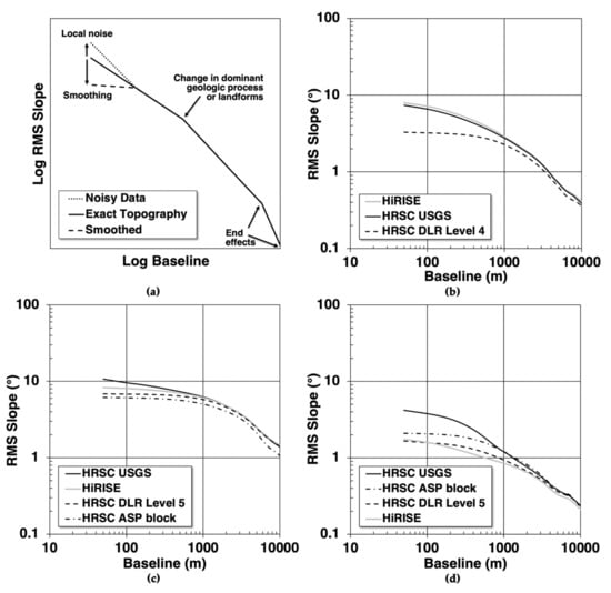
Figure 12.
RMS bidirectional slope as a function of baseline. (a) Schematic effects. (b) Gale data from [11]. (c) Data for Jezero crater rim area. (d) Data for Jezero crater floor. Data in c and d come from rectangular subareas within the red and green areas outlined in Figure 2, respectively.
Figure 12c shows north–south slopes averaged over a 3.35 × 12.8 km rectangle on the rim of Jezero crater, within the area outlined in red in Figure 2. (Results for CTX are not shown because the area analyzed is slightly different as a consequence of the different GSDs and the requirement that the Fourier transform length be a power of 2 posts.) As at Gale, the curve for the DLR DTM starts to depart from the HiRISE curve around 1500 m baseline and is flat for short baselines, with a “knee” around 490 m. The ratio of this transitional baseline to the optimal filter width is thus similar for both study areas. The curve for the ASP block matcher output (with optimum kernel sizes determined above) resembles that for the Level 5 product, but with slightly smaller slopes at all baselines. Slopes for the USGS HRSC DTM exceed those for HiRISE, indicating that the USGS DTM is noisy at baselines ≤1000 m. Though the HRSC DTM agrees best with HiRISE in elevation when the latter model is smoothed, such smoothing will clearly increase the discrepancy in slopes. Instead, better agreement with the true slope values can be had by smoothing the HRSC DTM slightly more. For example, smoothing the output of NGATE with a 5 × 5 lowpass boxcar filter rather than with AATE not only reduces the slope error at 50 m baseline (Figure 6), it yields a slope-baseline curve (not shown in Figure 12) that plots almost on top of the HiRISE curve. This agreement is partly fortuitous, since the slopes in the HiRISE model come almost entirely from real topography, whereas those in the HRSC DTM combine the effects of (smoothed) topography and errors, but because a consistent level of agreement is obtained over a range of baselines for terrains of varying roughness, it has practical value for applications such as landing site safety assessment.
Figure 12d shows data for an 8 × 12.8 km rectangle on the floor of Jezero crater, within the blue outline in Figure 2. Here, all three target DTMs examined overestimate slopes at intermediate and small baselines (<2000 m), indicating the presence of artifacts at these scales. All three curves also flatten somewhat at a baseline of between 300 and 500 m, indicating a deficiency of features smaller than this and supporting resolution estimates in this size range. The curve for the ASP DTM flattens so dramatically for baselines ≤300 m that the slope estimated at 50 m is nearly correct. The behavior of the USGS DTM is especially interesting. It indicates the presence of artifacts leading to increased slopes and stronger slope-baseline dependence over two ranges of baseline, a moderate effect at approximately 800–2000 m and a more pronounced increase over 300–800 m. As we discuss in the next section, the shaded relief portrayals of NGATE-derived DTMs, but not the others, appear to show populations of larger and smaller local bumps and hollows. Although slope errors on the Jezero floor are large in a relative sense, this is a smooth area and in absolute terms the errors are ≤2.5°, comparable to the data in Figure 12c.
3.4. Qualitative and Semiquantitative Assessments
Visual examination of the original and smoothed DTMs sheds additional light on the quantitative comparisons described in the previous section. Presenting the DTMs in the form of synthetic shaded relief images (Figure 13) emphasizes the local texture and details in which we are primarily interested. Examining the DTMs directly (as grayscale or color-coded images) leads to essentially the same conclusions. The inescapable first impression is that the target DTMs are substantially less detailed than the HiRISE data downsampled to the same GSD. For example, Figure 13a, the reference DTM resampled to 20 m/post but not smoothed, contains many small features not seen in the 20 m/post CTX DTM, Figure 13b. It is more instructive to compare each target DTM to its corresponding “best fit” smoothed reference DTM. Such pairs include Figure 13b–g,m. The target DTMs in Figure 13h–l all correspond to the reference Figure 13n. The CTX USGS and HRSC DLR Level 5 and ASP (block and SGM) DTMs each resemble their respective optimally smoothed HiRISE product quite closely. In particular, both the target and smoothed HiRISE DTMs appear homogeneous, with similar scales of detail in both the rugged western and smooth eastern areas. Close comparison shows that surfaces in the target DTMs appear slightly rougher than in the smoothed HiRISE data. This difference is particularly noticeable for CTX (Figure 13b,c).
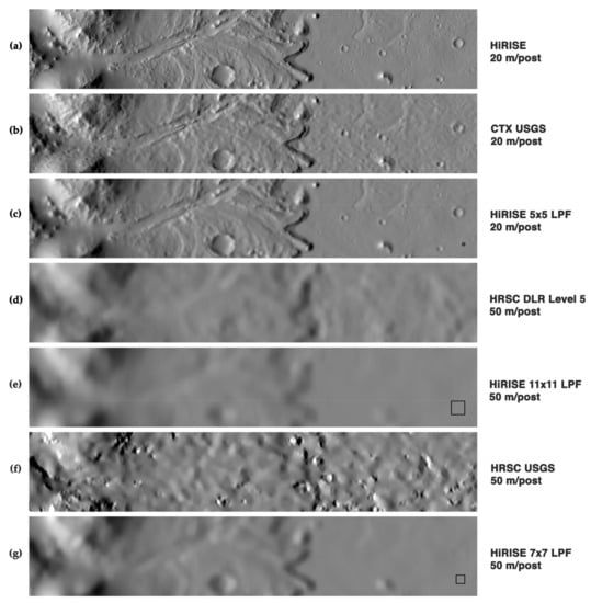
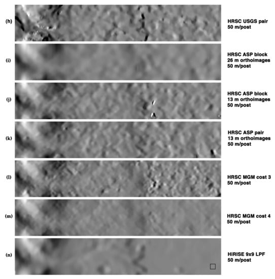
Figure 13.
Shaded relief portrayal of Jezero DTMs. (a) HiRISE downsampled to 20 m/post. (b) CTX at 20 m/post. (c) HiRISE at 20 m, smoothed 5 × 5 to match CTX (see Table 1). (d) HRSC DLR Level 5. This and the following parts of the figure are all at 50 m/post. (e) HiRISE at 50 m/post smoothed 11 × 11. (f) HRSC USGS. (g) HiRISE at 50 m/post, smoothed 7 × 7. (h) HRSC USGS, based on stereo channels only; compare to result f with stereo and nadir. (i) ASP block matcher (best kernel sizes). (j) ASP block matcher, nadir and stereo channels orthorectified at nadir GSD. (k) ASP block matcher, stereo channels only, orthorectified at nadir GSD. (l) ASP MGM cost mode 3. (m) ASP MGM cost mode 4. (n) HiRISE at 50 m/post, smoothed 9 × 9, best reference for DTMs h–l. Best reference form is HiRISE with 11 × 11 smoothing (e). All images 18 × 3.2 km, centered at 77.4° E, 18.5° N, Simple Cylindrical projection, north at top, latitude of true scale 18.6° N, illuminated from left with identical contrast stretch. HRSC products have been enlarged to aid comparison. Squares in panels (c,e,g,n) indicate the size of smoothing filter applied to HiRISE to match target DTM resolution. The largest crater is Belva, diameter 900 m.
The appearance of the HRSC USGS DTM is more complex. It contains features of similar size to those in the smoothed HiRISE reference, but also numerous smaller bumps and hollows. Regardless of their dimensions, many of these variations appear to be spurious (topographic “noise”) but some correspond to real surface features. These include some small features which are seen in the unsmoothed but not the smoothed HiRISE data. Some larger real features appear “broken up” into clusters of small humps in the HRSC DTM. A few relatively steep slopes (e.g., in the channel walls) appear to be resolved relatively accurately at widths as small as 150 m. On the other hand, the prominent 900 m diameter impact crater Belva in the center of the delta, which is subdued but visible in the DLR DTM, is almost entirely absent. All of these effects were also observed in the USGS DTM of the Gale crater T1 area [10,11]. The greater effective smoothness and reduced amplitude of errors in smoother terrain that we inferred from quantitative comparisons is not readily apparent to the eye. Using only the stereo channels in NGATE largely eliminated the smaller bumps and hollows seen in the DTMs produced from the triplet (cf. Figure 13f,h), corresponding to the increase (worsening) in estimated resolution.
The errors in the target DTMs take the form almost entirely of compact fluctuations (bumps and hollows) either at about the size of the best fit smoothing filter or, for the HRSC USGS DTM, at this size and smaller. The prominent pattern of correlated errors over small rectangular areas seen with the SOCET SET AATE matcher [32] was not observed in the DTMs produced with NGATE and smoothed with one AATE pass. Spikes or pits of amplitude exceeding local relief (indicating matching blunders) and gaps in the data caused by a lack of matched points were not observed in the Level 5 and NGATE DTMs. Some gaps were observed in DTMs from the ASP block matcher. In many cases, these were only obvious in the uninterpolated data, but interpolation between points with bad (high or low) elevations around the edges of gaps gave rise to spikes and pits in the DTM in some cases. The majority of these blunders occurred in areas where image quality was not conducive to matching, specifically in the shadow of the Jezero rim and on smooth areas and bedforms on the Jezero floor. Blunders on the crater floor were minimized in DTMs produced with the optimal kernel sizes, although a few remained in the HRSC DTMs based on orthoimages at the 13 m/pixel nadir GSD (Figure 13j,k) and in the best CTX DTM we were able to produce with ASP. Along the crater rim, blunders were common regardless of the source images or matcher parameters used. Despite the absence of obvious data gaps, surprisingly large features (e.g., Belva crater) were almost entirely absent from many of the DTMs. Figure 13l,m clearly illustrate the greater smoothing and lower noise level in smooth areas when the MGM algorithm is used with the ternary census transform (cost mode 4) compared to cost mode 3. A subtle, cloth-like pattern of artifacts is barely visible in Figure 13m but is more evident when a larger portion of the DTM is examined.
Heipke et al. [1] measured a quantity related to DTM resolution by counting impact craters visible in the shaded relief portrayal of the target DTM and in the corresponding orthoimage. The crater diameter at which half the craters identified in the image could be seen in the shaded DTM varied from 2 to 5 km for different processing approaches. The stereo channel GSD was 28 m, similar to our image set. We were unable to make useful crater counts because the small area of the Jezero study area set by the HiRISE coverage contains very few craters visible in the HRSC DTMs. This may be a consequence of the vertical precision as well as the horizontal resolution of the DTMs; the images show that the majority of craters present are degraded, with floors filled to nearly the surrounding level. Nevertheless, the few craters visible, along with some small knobs, provide bounds on the equivalent measure of resolution. The CTX DTM contains more craters, but rather than counting them we made a subjective assessment of the smallest craters and knobs that are reliably present.
The HRSC USGS DTM contains only one clear impact crater, with diameter 1800 m (just outside Jezero, hence not seen in Figure 13). Its rim is well resolved. As noted, Belva (900 m) is not visible. Knobs 500 m in diameter seen in the orthoimage are generally identifiable in the shaded relief (though many similar appearing bumps do not correspond to real features). Knobs 300 m in diameter are occasionally present, but those 200 m and smaller are generally not. In the HRSC DLR DTM, the 1800 m crater is visible, as is a 1600 m crater beyond the edge of the USGS coverage. Belva is visible but indistinct. Knobs as small as 600 m in diameter are visible; a few real knobs smaller than this can also be identified but appear to be ~600 m in width. In the CTX data, a great many small craters are seen in the shaded relief, but even more in the images. Some craters 150 m in diameter are distinguishable from noise in the elevation data, but many craters this size are not seen. At 300 m in diameter, most craters are visible. A few knobs as small as 50–70 m in diameter are visible but appear broadened to ~100 m. Thus, small features are blurred to approximately the scale of the optimal smoothing filter estimated above, and craters are sometimes visible at diameters 1.5× this smoothing width, but reliably visible at approximately 3× this size. Resolution as measured by crater visibility thus seems to lie at the low end of the range found by Heipke et al. [1]. This is unsurprising given that significant improvements have been made to both the DLR and USGS processing techniques in the interim [10,11,18].
Finally, we used two possible approaches to estimating vertical error that do not require a reference DTM and checked the quantitative agreement of these estimates with the reference-derived vertical errors described above. First, we collected elevation statistics for flat areas of the Jezero crater floor to make crude estimates of the vertical precision of the DTMs under the assumption that the dispersion in heights is dominated by matching errors rather than by real topography. The images and DTMs show areas that are topographically flat and level yet have abundant image texture as a result of albedo variations. The largest such rectangular area in the HRSC DTM was 7.5 × 3 km. The standard deviation of elevations in this box was 11.6 m for the DLR dataset and 12.2 m for USGS. In the CTX DTM, real topographic variations are apparent and the largest featureless box we could identify was 1 × 1 km. The elevation standard deviation was 2.64 m. If these elevation dispersions are attributed to matching error, the corresponding matching precisions are 0.296, 0.309, and 0.199 pixel, in reasonable to good agreement (+30%, +7%, −1%, respectively) with the results for the smooth area shown in Table 2. Second, we computed the RMS differences between pairs of target DTMs that we previously showed to have similar resolutions. The difference between overlapping DTMs has been used as a proxy for vertical precision where better reference data are unavailable (e.g., [44] and Bland et al., this issue). The reliability of the approach depends critically on the extent to which errors in the two DTMs are correlated. If the errors are perfectly correlated, they could be arbitrarily large yet the difference between the DTMs will be zero. At the other extreme, if the matching errors are statistically independent, then the RMS difference would be the root summed square of the expected vertical precisions, or √2 EP if the DTMs have similar precision. Table 4 shows the correlation coefficient between the errors (with respect to the best fitting smoothed reference DTM in each case), RMS difference, and EP estimates for three pairs of target DTMs that were selected to have similar estimated resolution. The DLR-NGATE and ASP block-NGATE comparisons (for the lowpass-filtered NGATE DTM with closest match in resolution) had similar correlation coefficients between errors. Using the RMS difference as a proxy will underestimate EP consistently but by less than 10% in these cases. The MGM model shows errors that are less correlated with those in NGATE, likely because the MGM algorithm is fundamentally different from the correlation method used in the other matchers but perhaps also in part because the resolutions are less well matched (the MGM model falls between two of the lowpass-filtered NGATE DTMs in resolution). Consistent with the lesser correlation, the difference between these DTMs overestimates their EP by 10–20%.
Table 4.
Differences between overlapping target DTMs compared to vertical precision EP.
4. Discussion
Because the majority of our results were obtained by using a reference DTM to estimate target DTM resolution and precision, we performed multiple tests to investigate the extent to which extraneous factors (listed below) might bias these estimates. The magnitude of such effects ranged from negligible to approximately the 10% level. First, regenerating the HRSC USGS DTM at 75 m/post rather than 50 m changed the estimated resolution very slightly (a 4% increase, or worsening, in resolution) but decreased the error by a similar amount, leaving the product of the two unchanged. Similarly, when we performed an independent analysis of the Level 5 and CTX DTMs by oversampling them by a factor of two, as well as using independent (non-ISIS) processing software, the resolution was within 10% and error within 5% of the values estimated for the same target DTM at its original GSD. This comparison was made with the DTMs trimmed to eliminate edge effects (a step omitted in producing our primary results), as discussed further below.
We also performed experiments by smoothing the HiRISE DTM with a Gaussian filter and recovering the “resolution” with boxcar filters as described above. Provided the Gaussian kernel is not truncated too tightly (the half-width of the finite kernel is at least 3-fold the width parameter σ, defined as the second moment for a one-dimensional Gaussian), the best-fit box width is approximately 3.6 σ. This corresponds closely to the ratio for which the second moment (weighted RMS radius) of the different kernels is the same, √2 σ for the two-dimensional Gaussian versus W/√6 for a two-dimensional boxcar of width W. Twice the second moment might thus be a useful way to express the width for filters with arbitrary kernel shapes, allowing the smoothing comparisons to be generalized. We note, however, that although the main characteristic of the boxcar filter that motivated its use was its simplicity, it does correspond directly to an idealized concept of a properly sampled DTM, in which the value of a pixel (post) represents an unweighted average of elevations within the area covered by that pixel. This concept applies to the reference DTMs we prepare by downsampling the 1 m/post HiRISE DTM to the GSD of the target, and if boxcar filters are used for smoothing it continues to apply to the smoothed reference DTMs. The filter size at which the error is minimized then addresses a very natural question: at what GSD would the target DTM have come closest to being an ideal representation of the area-averaged surface?
Any lowpass filter will introduce some inaccuracy into the smoothed DTM at the edges, where the kernel does not fully overlap the data. These errors, which are greater for larger filters, will bias the minimum difference toward smaller filter values, reducing the apparent resolution. The smoothed reference DTMs should therefore be trimmed by the halfwidth of the largest smoothing kernel to ensure that edge effects are eliminated (and that the area being compared is identical for all filters). The magnitude of the edge effect depends on the fraction of the DTM area affected, and thus on the filter width in comparison to the size of the DTM. It also depends on the amplitude of local relief at the scale of the resolution and will be somewhat greater for rougher terrains. We discovered that edge effects were significant for the narrow Gale T1 DTM while studying the photoclinometry results, and used appropriately trimmed reference DTMs for this part of the investigation. We did not redo the many comparisons for the Jezero dataset but performed spot checks that show that edge effects have less influence for this larger study area. Comparing results for the HRSC DTMs to the smoothed HiRISE data with and without trimming, we find that not trimming the reference DTMs decreases the apparent resolution by 6–12% (with larger effects for the smoother products) and changes the error by <1%. This was true for all matching algorithms. There is thus likely to be a bias on the order of 10% in our Jezero resolution results. The effect for CTX DTMs is even smaller (~3%) because of the smaller filter sizes in relation to the DTM area. The effect of trimming can thus be a significant fraction of the ~20% variation we found in the resolution-error product and should be kept in mind by future workers attempting to extend our results. Because it is a systematic effect that biases all our resolution (and resolution-error product) estimates, it does not alter our conclusions about how results for different datasets and processing approaches compare.
In the independent analysis described above in which the DTMs were oversampled by a factor of 2, however, edge effects were markedly greater, with resolutions underestimated by nearly a factor of 2 for HRSC and 1.25 for CTX. For both cameras, the trimmed results agree closely with results from our primary software for trimmed DTMs at the native GSD as reported above. Even closer agreement for resolution and error was obtained when we analyzed oversampled DTMs—either with and without trimming—with our primary and independent software. This agreement indicates that interpolating the DTMs, not the analysis software, is responsible for the increased edge effects. Thus, although we are confident that the results in our figures and tables for DTMs at native GSD are biased by only a small amount that does not alter our conclusions, the different behavior for oversampled DTMs serves as a warning that in any future work the smoothed reference DTMs should be trimmed to eliminate edge effects.
Horizontal misregistration has already been mentioned as a possible source of error in both the resolution and precision estimates. To quantify the effect of such misregistration, we repeated the analysis with the HRSC USGS DTM offset by one and two pixels from its nominal position in each cardinal direction. The RMS error at optimal smoothing showed a smooth minimum with respect to these offsets (Figure 14). Interpolating, we found that the best-fit position was 6.1 m west and 17.5 m north of the nominal location, for an overall error of 18.5 m (0.37 post). Fits to the results also yielded estimates of sensitivity of both the error and the resolution estimate (not shown in the figure) to small misalignments. A shift of one post (~2 pixels) increases both the optimal smoothing and the RMS error by ≤5%; two posts (4 pixels) of misregistration increases the values by ≤20%. Figure 14 shows that the error is a little more sensitive to east–west than to north–south shifts. This is readily understandable because the largest topographic feature in the study area is a segment of the Jezero rim with steep slopes to the east and west. Although this shows that the sensitivity to misregistration depends somewhat on the terrain, we anticipate that it will be generally similar for other areas with comparable slopes, including the Gale T1 DTM. We therefore conclude that registration errors as large as a few pixels (one pixel is more likely, based on the visual comparison of features) between our Gale DTMs may have led us to overestimate smoothing and precision by no more than 10–20%. This is consistent with the ~15% agreement between the Gale and Jezero results. Internal distortions in one of the DTMs being compared can potentially have a similar effect even when the datasets are perfectly aligned on average. As noted, the cross-track-scale discrepancy between the HRSC DTMs and the CTX base and the HiRISE mosaic adjusted to it has a RMS variation of 17 m across the HiRISE coverage, which is only a third of a post. The effect on resolution and error estimates should thus be a small fraction of a percent.
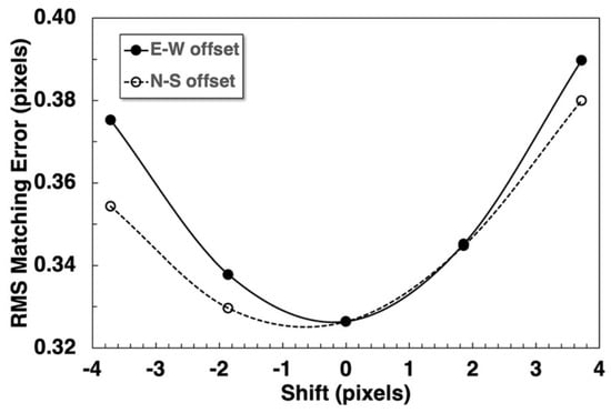
Figure 14.
RMS error (expressed as matching error ρ in pixels) as a function of small offsets of the HRSC USGS DTM relative to the best alignment to the reference DTM estimated by using pc_align. Shifts are scaled to the stereo channel image pixels, consistent with our presentation of normalized resolution and error. Measurements (symbols) were made by shifting the DTM a whole number of posts, and have been connected by smooth curves.
Vertical errors in registering the DTMs also play a role. We ignore the difference in mean elevations in each pair being compared (equivalent to adjusting them vertically to best mean agreement) but relative tilts will affect the difference statistics. The HRSC Level 5 DTM was found to have an approximately 0.1° tilt to the east relative to the other DTMs. Strictly speaking, the HRSC Level 5 DTM was controlled to MOLA so it is likely correct and the other DTMs are tilted relative to it. For purposes of our comparison, however, it was simpler to adjust the tilt of the Level 5 DTM rather than that of all the other products, which are consistent with one another. Subtracting a linear function of longitude from the Level 5 elevations reduced the RMS difference residuals and thus the error estimate for the DTM by 10%, with no effect on resolution. Again, vertical distortions internal to the DTMs can have a similar effect that is harder to correct. To analyze our CTX DTMs produced in ASP, where we were primarily concerned with changes in relative quality as a function of matcher parameters, we simply excluded the corners of the dataset that were most affected by jitter distortions from the comparisons. This decreased the RMS error estimate by approximately 15% but had no effect on the resolution or the kernel sizes at which the resolution was optimized.
5. Conclusions
Our strongest conclusion is qualitative: that comparing reference and target DTMs made from stereo images of very differing resolution provides a useful way to assess the resolution and precision of the lower-resolution target DTMs when—as is common in planetary exploration—ground data are not available for this purpose. Making such assessments, even for limited areas, allows us to measure and compare the quality of DTMs produced by different matching software, and to select parameters that yield the best DTM quality for a given matching approach. The required processing steps (apart from DTM generation) are simple, consisting of DTM alignment, spatial filtering, pixel algebra (subtracting one DTM from another) and collection of statistics, as shown in Figure 4. The results can be used both to assess the performance of a given stereo matching application and to guide the selection of parameter values to optimize that performance. Although we utilized reference DTMs generated at 20 to 50 times smaller post spacing than the target DTM, a smaller ratio would suffice to ensure that errors in the reference are negligible compared to those in the target data that are to be estimated.
We have obtained estimates for resolution (best-fit boxcar filter width of 10–20 image pixels) and error (matching precision ρ of 0.2–0.4 pixel) that vary by a factor of 2 for various images, terrains, and matching algorithms. This is significantly greater than any of the confounding effects discussed in the previous section, which introduced variations of ~10% or less. The range of results for vertical and image-matching precision is not unexpected. Although matching precision on the order of 0.2 pixel has long been a rule of thumb for predicting vertical precision (e.g., [45]), we have studied matching precision in SOCET SET (specifically, the USGS NGATE+AATE processing) with a variety of approaches applied to images from very different cameras [10,11,27,32,46] as well as synthetic images [5] and found values in the range 0.2–0.3 pixel. We have recommended this range as a rule of thumb for predicting vertical precision for particular images, and for designing stereo cameras and observations to meet some required precision. Matching errors greater than 0.3 pixel were found in the present study only for unsmoothed NGATE output and for ASP with kernel sizes far from the optimum or with subpixel matching turned off. None of these cases have been studied before and we do not envision situations in which they would be used. Our results for horizontal resolution are consistent with our past investigations based on reference DTMs [5,10,11]. These resolution estimates may be surprising because many DTMs are generated with a GSD between 3 and 5 image pixels. (For HRSC team products, GSD is set at approximately twice the mean image GSD which is often, as here, 4× the nadir GSD.) We have offered this as a rule of thumb for DTM design in past work (e.g., [5,27,32]) and justified it on the grounds that smaller GSD would not increase resolution. The rationale is that, for at least some matching tools, three pixels is the smallest (odd) patch size that could be used in area-based matching, so posts spaced more closely than this would not provide independent elevation information. Our results indicate that this lower limit is not violated, but also is not approached closely, at least when the average behavior over large regions is considered. One possible explanation for the discrepancy is that matching software may choose patch sizes larger than the minimum possible. We have seen evidence for such an internal limit on resolution in SOCET SET: whereas the resolution of DTMs produced from images at their native GSD was ~15 pixels, DTMs made from images that had been oversampled could approach a resolution of 4-fold the original GSD. Another possibility, not mutually exclusive, is that the kernel for area-based matching does not act simply as a lowpass filter, averaging parallax (thus elevation) information over its domain. This idea is supported by our present results for the ASP block matcher, for which DTM resolution increases only fractionally when the kernel size is increased to twice its optimum value or more (Figure 8).
An important aspect of our results is that DTM resolution and precision do not vary independently by factors of 2. Rather, they are approximately inversely correlated. Excluding methods that are unlikely to be used in practice (e.g., unsmoothed NGATE, block matching without subpixel refinement), our results for the product of resolution and error are almost all within 20% of the best case across multiple terrains and algorithms (Table 5). In absolute terms, these results are mostly in the range of 4–5 pixels squared, compared to ~1 pixel squared if 0.2–0.3 pixel matching precision could be obtained simultaneously with 3–5 pixel resolution.
Table 5.
Relative variation of the resolution-error product for Jezero DTMs.
In dramatic contrast to the range of stereo results in Table 5, refining the Gale T1 DTM by photoclinometry resulted in quality improving by tens of percent. For the subarea with the most uniform albedo, the product of resolution and error was reduced to 0.44 of the starting (NGATE + AATE) value, and resolution was improved to 0.39 of the starting value. The uncorrected albedo variations that led to less dramatic improvement (or, in extreme cases, degradation) of the DTM in other areas were generally evident in the image both before and after albedo-correction based on the stereo DTM. Given that artifacts in photoclinometric DTMs start as local tilts at albedo features and “grow” into stripes as iteration proceeds [32,39], stopping the iteration at an appropriate point will limit the impact on nearby topographic features. Thus, many of the details in even a less-favorable part of the DTM may be enhanced significantly, even though the quality in an RMS sense is less improved.
We have also attempted to assess DTM quality by methods that do not require a reference DTM, both to corroborate our primary results and to determine how DTMs might be assessed in the general case where no reference is available. Elevation dispersions in flat areas (identified in the target DTM and orthoimage) agree closely with our primary estimates of vertical precision. The RMS difference between target DTMs of similar resolution was also found to be within 10% of the error estimate based on the reference DTM in the cases we examined. We looked at DTMs made from the same images with different algorithms, so similar results may be expected where (say) SOCET SET and ASP DTMs of Europa are compared ([44] and paper by Bland et al. in this issue). Caution is needed in extrapolating to cases where it is desired to compare overlapping DTMs produced from different images with the same software, especially because the resolution of the images and thus the DTMs may be quite different.
Because we have used such disparate approaches to try to quantify the horizontal resolution of the target DTMs, it is appropriate to discuss what is meant by the term (we exclude at the outset the erroneous usage of resolution as a synonym for pixel size or GSD) and how the different measures are expected to compare. In contemporary usage (e.g., [47]), resolution is usually defined as the size of a minimally discernable gap between features, or a line. (Earlier usage referred instead to the separation between centers of features, equal to a line pair.)
Smoothing with a lowpass boxcar filter will attenuate signals with a wavelength equal to the filter width while passing longer-wavelength signals. Although the peak-to-peak wavelength is equivalent to the separation rather than the gap between features (i.e., a line pair), it must be bigger than the filter width to be visible. Thus, the width of the smallest resolvable line or other feature is likely to be close to the filter width, and this is what we observe in comparing the broadened appearance of small knobs to the amount of smoothing inferred from comparing target and reference DTMs. As noted above, visual assessment does not resolve differences as small as 10% in the apparent size of features, much less the subtle differences in appearance that might result from smoothing with functions of comparable width but different shapes. Thus, the range of our quantitative results (e.g., based on different filter shapes or resampling DTMs to different GSD) are all consistent with what the eye can discriminate.
Slopes are computed for a discrete baseline, and should be just detectable when that baseline extends from (say) the top of a local high to the floor of a barely resolved adjacent gap; this is equivalent to the resolvable line width. “Resolution” defined by the diameter of an identifiable crater requires more thought. At a minimum, the diameter might be equivalent to the width of a line pair, for a simple craterform defined by a high–low–high pattern of elevations. Recognition of a landform such as a crater is usually taken to require at least 3 to 5 resolution elements. Thus, we would expect detected craters to be at least as large as the optimal smoothing, and possibly 2- or 3-fold larger. Considered in this light, the various resolution estimates for each Gale and Jezero dataset are mutually consistent. Though our work shows the value of a reference dataset for evaluating DTM quality, this consistency indicates that rough but useful quality estimates can be obtained without such a reference if the terrain contains discrete features with a range of sizes.
Perhaps our most surprising result is the spatially variable quality of the USGS DTMs. Not only do the precision and best-fit smoothing vary with roughness, individual areas contain a mixture of features (and noise) ranging from the size of the best-fit filter to much smaller. These variations make sense in light of the description [28,29] that the NGATE matcher produces a dense set of candidate matches and then filters them in a robust way to populate the output DTM. The details are proprietary, but it is plausible that the algorithm applies more smoothing (yielding smaller precisions) when it detects smoother terrain. It seems also to apply a mix of stronger and weaker smoothing locally, resulting in the mix of relief at multiple scales. Why the precision was terrain sensitive for CTX data, but the smoothing was not, is unclear. The obvious differences between CTX and HRSC images are the higher signal-to-noise ratio and smaller GSD of the former. Perhaps higher resolution allows CTX to detect and match localized, high contrast albedo variations. An abundance of matchable features might explain why the resolution is consistent but we would expect it to be consistently good whereas it seems to be consistently slightly worse than for HRSC. The HRSC DLR Level 5 DTM is more homogeneous in both resolution and error, indicating a different and less terrain-sensitive processing approach. Note that smoothing the NGATE DTM with an appropriately chosen filter yields resolution and error very close to those of the Level 5 product on average, but the greater roughness dependence of NGATE is still detectable.
Our results lead to several recommendations addressed to DTM producers and users.
- A reminder that resolution is not the same as pixel size (GSD) is always in order. The distinction is even more important for DTMs than for images.
- Those who design cameras and investigations to address scientific questions should be aware of not only the ranges of resolution and precision that can be expected for DTMs made from stereopairs of a given GSD, but the combinations of resolution and precision that are achievable simultaneously. The value of 4–5 pixels squared for the product of DTM resolution and matching error is a useful rule of thumb.
- For producers of stereo DTMs, 3–5 image pixels is still a good rule of thumb for selecting the post spacing. Our results indicate that following this guideline is almost certain to oversample the data.
- Because our investigation showed only fractional differences in the combined figure of merit (the product of resolution and error) among several matching approaches, stereo DTM producers may want to concentrate on achieving their desired tradeoff between resolution and error rather than searching for the matcher that produces the best product of the two. Additional research is nevertheless needed into developing and improving matching algorithms or into assessing the resolution, error, and the product of these for additional types of matchers.
- Multiple approaches to smoothing the output of the NGATE matcher gave nearly identical results. We recommend that SOCET SET/GXP users use either an AATE pass or a 5 × 5 lowpass boxcar filter, either of which yields near-optimal resolution-error product and resolution-slope accuracy tradeoff. Although greater smoothing may be desired for some applications, this can easily be applied after the fact.
- For ASP users, block matching with a 13 pixel subpixel refinement kernel is recommended as likely to be near-optimal. The normalized cross-correlation kernel needs to be “big enough” to minimize blunders. The minimum acceptable NCC kernel size likely depends on details of the images used, so some experimentation with this parameter may be needed. The SGM/MGM algorithms did not offer significant advantages over block matching for our images, but they might in other situations. In particular, using these methods with the ternary census model (cost mode 4) did result in the lowest errors on the Jezero crater floor and might be preferred for mapping very smooth terrains.
- Including the HRSC nadir channel image improved DTM resolution and precision in SOCET SET but not to a significant degree in ASP. Nevertheless, we recommend using all three images even in ASP because doing so reduced the occurrence of interpolated holes in the matching point cloud. Computing the intersection of more than two image rays has been found to have beneficial effects on both reducing and estimating (through the intersection error map) DTM errors in the HRSC stereo pipeline at DLR [21]. The ASP manual [33] states that the multi-view intersection capability “somewhat experimental, and not used widely. We have obtained higher quality results by doing pairwise stereo and merging the result ….” It may therefore be appropriate to reexamine the performance of ASP with multiple images when the multi-view capability has matured.
- Photoclinometry should be considered as a viable method for improving DTMs beyond the resolution and error achievable by stereo matching alone. DTMs produced ab initio by photoclinometry (i.e., not starting with a stereo product) formed an important component of Mars landing site selection before the availability of HiRISE images for this reason [27,32]. For single-image photoclinometry [39] to be useful, the image should not contain albedo variations visible to the eye. Albedo variations at scales resolved by the stereo DTM can be corrected by straightforward image processing [10,11]. The true resolution of the DTM provides a guide to how many iterations should be performed before stopping the photoclinometry algorithm. The stopping point should in the range of 2–4-fold the ratio of the DTM resolution to the GSD of the image being processed. Because we tested the use of photoclinometry by using an orthoimage at the same pixel spacing as the stereo DTM, we used the GSD of the DTM (and our orthoimage) in this calculation. If an orthoimage with a smaller GSD (e.g., matching the raw image) is used, more iterations would be needed.
- Users of DTMs produced in SOCET SET should be especially careful in interpreting DTM resolution estimates, which at best are averages over complex behavior. The DTMs can be expected to contain bumps and hollows at a range of sizes larger and smaller than the resolution estimated by comparison to a reference DTM (if one is available), and these will be a mixture of real features and artifacts. Estimating resolution based on the appearance of DTM or shaded relief is difficult. Resolution and precision will vary within a given DTM as a function of surface slopes, and depend on the smoothing applied when the DTM was produced. If the smoothing recommended above (AATE or 5 × 5 lowpass filter) was used, slopes are likely to be within a few degrees of the correct value at all baselines. If avoiding misinterpreting small artifacts as surface features is more important than slope accuracy, users should smooth DTMs with a lowpass filter before use.
Future Work
These conclusions open up numerous possible lines of investigation. As a practical matter, can the quality of stereo DTMs produced with the packages we investigated be improved further? We have treated the DLR pipeline as a fixed entity so far, which was reasonable given the thousands of HRSC DTMs that have been delivered to the ESA Planetary Science Archive and NASA Planetary Data system. The standard Level 4 [21] and Level 5 processing [18] were optimized based on extensive testing, but comparing their output to HiRISE reference DTMs would likely allow the identification further improvements. In SOCET SET and GXP there are aspects of NGATE beyond smoothing of the final result that can be controlled by choosing or even editing “strategy” files. SOCET GXP also includes a new matching module, Automated Spatial Modeler (ASM). Although ASM was partly designed to improve the speed of the matching algorithms in NGATE, it combines these with additional methods including SGM [48], and it would therefore be of interest to quantify its performance with planetary data. ASP offers many features such as filtering of the DTMs that we have not tested. As noted above, the multi-image intersection capability in ASP is still experimental, so it would be of interest to compare the results of collecting and merging multiple point clouds from pairwise matching, and to reassess the multi-ray intersection capability when it has matured. Adaptive spatial filtering of the images before matching contributes significantly to the effectiveness of the DLR pipeline [21] and could be explored in conjunction with SOCET SET/GXP and ASP. Work now underway at the USGS to provide a more complete and user-friendly interface between ISIS, ASP, and SOCET SET would also open up new possibilities for using ASP and SOCET SET or GXP together. For example, in this investigation, we were not able to make use of the jitter-corrected orientation data for CTX at Jezero because tools for transferring such support data have yet to be created. As a result, we had to do an independent bundle adjustment of a CTX stereopair to use it in ASP. The result was a DTM with jitter distortions relative to the CTX mosaic produced with SOCET SET. Full interoperability of the packages would also make it possible to produce DTMs in ASP with minimal interactive work and investigate whether using them as a “seed” for NGATE or even editing them interactively in SOCET SET or GXP could yield higher quality DTMs (as quantified by the approach described here) with less effort than our current procedures.
In addition to further work with these packages, of course, it will be of interest to evaluate other matching approaches as software implementations that handle planetary images become available or processed DTMs are released. A prominent example is the CASP-GO system [49], which utilizes ASP and elements of ISIS but also includes subpixel refinement by the Gotcha algorithm [50]. Unfortunately, the CASP-GO CTX DTMs available at the time of this investigation only included partial coverage over our Jezero reference dataset. The Ames Stereo Pipeline development team has implemented a plug-in interface to allow use of third-party code for other matching algorithms in ASP and is currently working on making the elements that CASP-GO adds to the ASP workflow, which are not limited to an image matching module, available (R. Beyer, oral comm. at 5th Planetary Data Workshop and 2nd Planetary Science Informatics & Data Analytics meeting, 2 July 2021). These developments have the potential to increase the range of matching approaches that could be tested by the methods of this paper.
Another direction for future research would be to apply the matching tools used in this paper to a wider range of images. Under what circumstances are the quality estimates and optimal parameters reported here still applicable, and how and when might they need to be modified? An obvious starting point for such an investigation would be to compare results where HiRISE reference DTMs cover more diverse Martian terrains. Comparison of results on other bodies would provide an even stronger test of the effect of terrain characteristics. The Moon is the most suitable place (after Mars) for such comparisons, because the Lunar Reconnaissance Orbiter Narrow Angle Camera (LROC NAC; [51]) has obtained numerous 0.5–2.0 m/pixel stereopairs. Existing [52] or new DTMs made from these pairs could be used as the reference against which to evaluate DTMs from the many other, lower-resolution lunar cameras. Europa is another intriguing target, in part because plans for the Europa Imaging System (EIS) cameras on NASA’s Europa Clipper spacecraft include extensive stereo imaging and DTM production [53]. Stereo image coverage of Europa currently available from prior missions such as Galileo does not support the kind of reference-target comparison described here, but the qualitative assessment of ASP performance ([44] and paper by Bland et al. in this issue) is extremely intriguing. They produced DTMs with a range NCC and SP kernel sizes in all combinations. Their visual assessment, that the NCC kernel size had little effect but that increasing SP kernel size resulted in smoother DTMs, is entirely consistent with our results for SP kernels equal to or larger than the optimum. Bland et al. only investigated SP kernel sizes between 15 and 45 pixels. Extending their tests to smaller kernels would reveal, even without a reference DTM, whether there is an optimum SP kernel size below which the DTMs become much noisier. If so, is this optimum size 13 pixels on Europa, as we found it to be in effectively all tests on Mars?
In addition to evaluating the quality of DTMs on different terrains and bodies, our methodology could be used to address more focused questions about the effects of scene content. How do DTM resolution and precision degrade with decreasing SNR, varying image sharpness (i.e., point-spread function), lossy data compression, or (for cameras that, unlike HRSC, do not acquire both images of a pair simultaneously) with illumination differences? The first three effects could be addressed by degrading planetary images in controlled ways and to varying extents. We investigated the effect of illumination through the use of synthetic images [5] but it would be valuable to confirm that similar results apply to real images. Images and stereopairs of the same region obtained with different illumination directions are available in the polar regions of Mars and the Moon.
Our results to date are based on a comparison of gridded DTMs, which are derived products interpolated from the point clouds that are the direct output of image matching and ray intersection. Direct assessment of the two-dimensional density of points, including its variations with surface texture, as well as resolution and vertical errors in such point clouds is therefore desirable and could point to ways to further improve stereo mapping accuracy. At a minimum, such a study would help to disentangle the influence of the matching algorithms and their parameters from effects introduced during interpolation and gridding. The error in ray intersection is a quality parameter that is defined for individual points (though it can be interpolated to the DTM grid) that might be useful to consider in conjunction with reference-target elevation differences. SOCET SET/GXP do not provide access to stereo point cloud data or intersection error, but the noncommercial DLR pipeline and ASP software packages do. With a native GSD of 1 m, HiRISE DTMs should be as useful for evaluating point clouds as they are for DTMs.
Given that we found uncorrected albedo variations a significant obstacle to refining stereo DTMs with single-image photoclinometry, can better results be obtained with a multi-image approach that solves for both albedo and topography? Numerous formulations of the problem have been described, one of which [54] is available in ASP in a form compatible with HRSC and other planetary images. Whether this capability can be tested at Jezero will depend on the availability of additional images with illumination sufficiently different from that in the HRSC observation (h5270_0000) used here. The Moon may be a more favorable body on which to conduct initial tests, because of the absence of atmospheric scattering effects on the images. Again, sets of images with the wide range of illumination directions that is needed are most available at high latitudes. The challenge will be to find an appropriate combination of reference and target data.
Finally, although we have shown that high-resolution reference DTMs are useful research tools for testing matching algorithms and optimizing parameters, they have limited value for certifying the quality of DTMs in routine production because they are available only for limited areas. It would be highly desirable to identify or construct indicators of quality that do not require a reference, especially local quality metrics that could guide the interpretation of bumps and hollows in the DTM as either real geomorphology or mapping artifacts. The software packages used here provide information qualitatively related to errors, but not quantitative estimates of DTM precision. ASP outputs a binary “good pixel map” that simply marks pixels as successfully matched or not and a map of ray intersection error. Intersection error is also computed in the DLR pipeline. The “figure of merit” (FOM) file from NGATE combines flag values for special cases (e.g., where DTM values were interpolated for reasons such as excessive slope or were manually edited) with correlation values for most posts. We have found these products to have limited utility. In most cases only a few posts are “bad” or interpolated. Blunders by the ASP block matcher (and DLR software) are often flagged by large intersection errors, and this connection is particularly evident in extended problem areas (e.g., the shadowed side of the Jezero rim). Most posts, however, have low intersection errors (DLR and ASP) or high correlations (NGATE). Thus, most local undulations seem to be statistical inliers, variations within the vertical precision of successful image matching, rather than cases of poor or failed matching. In our experience, the best way to assess the reality of individual small “features” in a DTM is to compare a terrain shaded relief to the orthoimage. This is essentially a binary classification; the orthoimage may show, for example, that a dimple in the DTM corresponds to an identifiable impact crater in the orthoimage, but this provides no information about how accurately the depth of the crater has been measured. A desirable goal would thus be to develop more quantitative estimators of local DTM precision from these qualitative indicators or others such as image texture metrics. High-resolution reference DTMs of select areas are likely to be essential for calibrating and validating any such estimators.
Author Contributions
Conceptualization, R.L.K.; methodology, R.L.K., K.G. and D.P.M.; software, D.P.M., T.M.H. and K.G.; photogrammetric data processing, B.L.R., D.M.G., D.P.M. and K.G.; photoclinometry processing R.L.K.; analysis, R.L.K. and K.G.; writing—original draft preparation, R.L.K.; writing—review and editing, K.G., D.P.M., R.L.F. and T.M.H.; supervision, R.L.F.; project administration, R.L.K. and K.G.; funding acquisition, R.L.K., R.L.F. and K.G. All authors have read and agreed to the published version of the manuscript.
Funding
Work conducted at the U.S. Geological Survey (USGS) was funded by the National Aeronautics and Space Agency (NASA) Mars Express Project, the NASA Planetary Geology and Geophysics Cartography program (2005–2015) and the NASA-USGS Interagency Agreement for planetary spatial data infrastructure (2016–present). HRSC work by Gwinner was supported by funding from the German Aerospace Center (DLR).
Data Availability Statement
Source data, including all images and reference DTMs, used in this study are publicly available for digital download from the European Space Agency Planetary Science Archive (PSA), the National Aeronautics and Space Administration Planetary Data System (PDS) Imaging Science and Cartography and HiRISE nodes, the U.S. Geological Survey (USGS), and the German Aerospace Center (DLR). DTMs produced in SOCET SET and the Ames Stereo Pipeline exclusively for the purposes of evaluation in this study are not considered deliverables because only summary statistics from them were used. HiRISE and CTX images (PDS): https://pds-imaging.jpl.nasa.gov/volumes/mro.html (accessed 1 September 2021). Search page for HRSC products including images and single-orbit DTMs (PSA): https://archives.esac.esa.int/psa/#!Table%20View/HRSC=instrument (accessed 1 September 2021). Duplicate archive of HRSC data, not current (PDS). https://pds-geosciences.wustl.edu/mex/mex-m-hrsc-3-rdr-v3/mexhrs_1001/ (accessed 1 September 2021) for images and https://pds-geosciences.wustl.edu/mex/mex-m-hrsc-5-refdr-dtm-v1/mexhrs_2001/ (accessed 1 September 2021) for single orbit DTMs. HRSC Level 5 MC DTMs and orthoimages (DLR) http://hrscteam.dlr.de/HMC30/index.html (accessed 1 September 2021). Mars 2020 landing site products (USGS; the respective orthomosaics are linked from these pages): CTX DTM mosaic https://astrogeology.usgs.gov/search/map/Mars/Mars2020/JEZ_ctx_B_soc_008_DTM_MOLAtopography_DeltaGeoid_20m_Eqc_latTs0_lon0 (accessed 1 September 2021). HiRISE DTM mosaic https://astrogeology.usgs.gov/search/map/Mars/Mars2020/JEZ_hirise_soc_006_DTM_MOLAtopography_DeltaGeoid_1m_Eqc_latTs0_lon0_blend40 (accessed 1 September 2021). HiRISE DTMs (PDS): https://www.uahirise.org/dtm/ (accessed 1 September 2021). In particular the Gale T1 DTM is available at https://www.uahirise.org/dtm/dtm.php?ID=PSP_009149_1750 (accessed 1 September 2021). Software: ISIS software and documentation are available at https://github.com/USGS-Astrogeology/ISIS3 (accessed 1 September 2021). Additional documentation is available at https://isis.astrogeology.usgs.gov/ (accessed 1 September 2021). Software for transferring planetary data between ISIS and SOCET SET and a detailed tutorial for producing DTMs from HiRISE images are available at https://github.com/USGS-Astrogeology/socet_set (accessed 1 September 2021). The commercial off-the-shelf stereo software used in some of the research reported here, SOCET SET, is no longer available from BAE Systems. The current system, SOCET GXP, includes the stereo matching modules from SOCET SET. The USGS Astrogeology Science Center is in the process of transitioning to GXP for planetary stereomapping. This process includes converting the relevant camera models to the Community Sensor Model (CSM) standard used by GXP (and other software packages), implementing the ISIS-GXP data interface, and developing workflows and documentation. CSM sensor model code are available at https://github.com/USGS-Astrogeology/usgscsm (accessed 1 September 2021). An environment for testing these models is available at https://github.com/USGS-Astrogeology/knoten (accessed 1 September 2021), with examples at https://github.com/USGS-Astrogeology/usgscsm/wiki/CSM-Stereo-Testing-Examples (accessed 1 September 2021). Scripts and other information helpful for DTM production with GXP are available at https://github.com/USGS-Astrogeology/APPL-Tools (accessed 1 September 2021). These resources are updated frequently. Software and extensive documentation for ASP are available at https://github.com/NeoGeographyToolkit/StereoPipeline (accessed 1 September 2021).
Acknowledgments
We thank the HRSC Experiment team at the DLR Institute of Planetary Research, Berlin, and at Freie Universität Berlin, the HRSC Science Team, and the Mars Express Project teams at ESTEC, ESOC, and ESAC for their successful planning and acquisition of data as well as for making processed data available to the HRSC team. Any use of trade, firm, or product names is for descriptive purposes only and does not imply endorsement by the U.S. Government.
Conflicts of Interest
The authors declare no conflict of interest.
References
- Heipke, C.; Oberst, J.; Albertz, J.; Attwenger, M.; Dorninger, P.; Dorrer, E.; Ewe, M.; Gehrke, S.; Gwinner, K.; Hirschmüller, H.; et al. Evaluating planetary digital terrain models—The HRSC DTM test. Planet. Space Sci. 2007, 55, 2173–2191. [Google Scholar] [CrossRef]
- Smith, D.E.; Zuber, M.T.; Frey, H.V.; Garvin, J.B.; Head, J.W.; Muhleman, D.O.; Pettengill, G.H.; Phillips, R.J.; Solomon, S.C.; Zwally, H.J.; et al. Mars Orbiter Laser Altimeter: Experiment summary after the first year of global mapping of Mars. J. Geophys. Res. 2001, 106, 23689–23722. [Google Scholar] [CrossRef]
- Neukum, G.; Jaumann, R. HRSC: The High Resolution Stereo Camera of Mars Express. In Mars Express: The Scientific Payload (ESA SP-1240); ESA Publications Division, ESTEC: Noordwijk, The Netherlands, 2004; pp. 17–35. [Google Scholar]
- Craft, K.L.; Barnouin, O.S.; Gaskell, R.; Palmer, E.; Weirich, J.; Perry, M.; Bierhaus, B.; Norman, C.; Huish, D.; Olds, R.; et al. Assessing stereophotoclinometry by modeling a physical wall representing asteroid Bennu. Planet. Space Sci. 2020, 193, 105077. [Google Scholar] [CrossRef]
- Kirk, R.L.; Howington-Kraus, E.; Hare, T.M.; Jorda, L. The effect of illumination on stereo DTM quality: Simulations in support of Europa exploration. ISPRS Ann. Photogramm. Remote Sens. Spat. Inf. Sci. 2016, III-4, 103–110. [Google Scholar] [CrossRef]
- McEwen, A.S.; Eliason, E.M.; Bergstrom, J.W.; Bridges, N.T.; Hansen, C.J.; Delamere, W.A.; Grant, J.A.; Gulick, V.C.; Herkenhoff, K.E.; Keszthelyi, L.; et al. Mars Reconnaissance Orbiter’s High Resolution Imaging Science Experiment (HiRISE). J. Geophys. Res. 2007, 112. [Google Scholar] [CrossRef]
- Malin, M.C.; Bell, J.F.; Cantor, B.A.; Caplinger, M.A.; Calvin, W.M.; Clancy, R.T.; Edgett, K.S.; Edwards, L.; Haberle, R.M.; James, P.B.; et al. Context Camera Investigation on board the Mars Reconnaissance Orbiter. J. Geophys. Res. 2007, 112. [Google Scholar] [CrossRef]
- Golombek, M.; Grant, J.; Kipp, D.; Vasavada, A.; Kirk, R.L.; Fergason, R.; Bellutta, P.; Calef, F.; Larsen, K.; Katayama, Y.; et al. Selection of the Mars Science Laboratory Landing Site. Space Sci. Rev. 2012, 170, 641–737. [Google Scholar] [CrossRef]
- Kirk, R.L.; Howington-Kraus, E.; Galuszka, D.; Redding, B.; Antonsen, J.; Coker, K.; Foster, E.; Hopkins, M.; Licht, A.; Fennema, A.; et al. Near-complete 1-m topographic models of the MSL candidate landing sites: Site safety and quality evaluation. Eur. Planet. Sci. Conf. 2011, 6, EPSC-DPS2011–1465. [Google Scholar]
- Kirk, R.L.; Howington-Kraus, E.; Edmundson, K.; Redding, B.; Galuszka, D.; Hare, T.; Gwinner, K. Community tools for cartographic and photogrammetric processing of Mars Express HRSC images. Int. Arch. Photogramm. Remote Sens. Spat. Inf. Sci. 2017, 42, 69–76. [Google Scholar] [CrossRef]
- Kirk, R.L.; Howington-Kraus, E.; Edmundson, K.; Redding, B.; Galszka, D.; Gwinner, K. Community tools for cartographic and photogrammetric processing of Mars Express HRSC images. In Planetary Remote Sensing and Mapping; Wu, B., Di, K., Oberst, J., Karachevtseva, I.P., Eds.; Taylor & Francis: Abingdon, UK, 2018; pp. 107–124. [Google Scholar]
- Fergason, R.L.; Hare, T.M.; Mayer, D.P.; Galuszka, D.M.; Redding, B.L.; Cheng, Y.; Otero, R.E. Mars 2020 Terrain Relative Navigation support: Digital terrain model generation and mosaicking process improvement. In Proceedings of the 4th Planetary Data Workshop, Flagstaff, AZ, USA, 18–20 June 2019; LPI Contribution 2151. p. 7047. [Google Scholar]
- Fergason, R.L.; Hare, T.M.; Mayer, D.P.; Galuszka, D.M.; Redding, B.L.; Smith, E.D.; Shinaman, J.R.; Cheng, Y.; Otero, R.E. Mars 2020 Terrain Relative Navigation flight product generation: Digital terrain model and orthorectified image mosaic. Lunar Planet. Sci. 2020, 51, 2020. [Google Scholar]
- Kirk, R.L.; Fergason, R.L.; Redding, B.; Galuszka, D.; Smith, E.; Mayer, D.; Hare, T.M.; Gwinner, K. Evaluating stereo DTM quality at Jezero crater, Mars with HRSC, CTX, and HIRISE images. Int. Arch. Photogramm. Remote Sens. Spat. Inf. Sci. 2020, 43, 1129–1136. [Google Scholar] [CrossRef]
- Kirk, R.L.; Mayer, D.; Redding, B.L.; Galuszka, D.M.; Fergason, R.L.; Hare, T.M.; Gwinner, K. Further adventures in Mars DTM quality: Smoothing errors, sharpening details. Int. Arch. Photogramm. Remote Sens. Spat. Inf. Sci. 2021, 43, 659–666. [Google Scholar] [CrossRef]
- Beyer, R.A.; Alexandrov, O.; McMichael, S. The Ames Stereo Pipeline: NASA’s open source software for deriving and processing terrain data. Earth Space Sci. 2018, 5, 537–548. [Google Scholar] [CrossRef]
- Gwinner, K.; Oberst, J.; Jaumann, R.; Neukum, G. Regional HRSC multi-orbit digital terrain models for the Mars Science Laboratory candidate landing sites. Lunar Planet. Sci. 2010, 41, 2727. [Google Scholar]
- Gwinner, K.; Jaumann, R.; Hauber, E.; Hoffmann, H.; Heipke, C.; Oberst, J.; Neukum, G.; Ansan, V.; Bostelmann, J.; Dumke, A.; et al. The High Resolution Stereo Camera (HRSC) of Mars Express and its approach to science analysis and mapping for Mars and its satellites. Planet. Space Sci. 2016, 126, 93–138. [Google Scholar] [CrossRef]
- Kersten, E.; Gwinner, K.; Michael, G.; Dumke, A.; Jaumann, R. Topographic mapping of the Mars MC quadrangles using HRSC data. EGU Gen. Assem. 2021, 23, EGU21–2745. [Google Scholar]
- Gwinner, K.; Scholten, F.; Preusker, F.; Elgner, S.; Roatsch, T.; Spiegel, M.; Schmidt, R.; Oberst, J.; Jaumann, R.; Heipke, C. Topography of Mars from global mapping by HRSC high-resolution digital terrain models and orthoimages: Characteristics and performance. Earth Planet. Sci. Lett. 2010, 294, 506–519. [Google Scholar] [CrossRef]
- Gwinner, K.; Scholten, F.; Spiegel, M.; Schmidt, R.; Giese, B.; Oberst, J.; Heipke, C.; Jauman, R.; Neukum, G. Derivation and validation of high-resolution digital terrain models from Mars Express HRSC-data. Photogramm. Eng. Remote Sens. 2009, 75, 1127–1142. [Google Scholar] [CrossRef]
- Sides, S.C.; Becker, T.L.; Becker, K.J.; Edmundson, K.L.; Backer, J.W.; Wilson, T.J.; Weller, L.A.; Humphrey, I.R.; Berry, K.L.; Shepherd, M.R.; et al. The USGS Integrated Software for Imagers and Spectrometers (ISIS 3) instrumentsupport, new capabilities, and releases. Lunar Planet. Sci. 2017, 48, 2739. [Google Scholar]
- USGS-Astrogeology/ISIS3. Available online: https://github.com/USGS-Astrogeology/ISIS3 (accessed on 1 July 2021).
- Miller, S.B.; Walker, A.S. Further developments of Leica digital photogrammetric systems by Helava. ACSM/ASPRS Annu. Conv. Expo. Tech. Pap. 1993, 3, 256–263. [Google Scholar]
- Miller, S.B.; Walker, A.S. Die Entwicklung der digitalen photogrammetrischen Systeme von Leica und Helava. Z. Photogramm. Fernerkund. 1995, 63, 4–16. [Google Scholar]
- USGS-Astrogeology/Socet_Set. Available online: https://github.com/USGS-Astrogeology/socet_set (accessed on 1 July 2021).
- Kirk, R.L.; Howington-Kraus, E.; Rosiek, M.R.; Anderson, J.A.; Archinal, B.A.; Becker, K.J.; Cook, D.A.; Galuszka, D.M.; Geissler, P.E.; Hare, T.M.; et al. Ultrahigh resolution topographic mapping of Mars with MRO HiRISE stereo images: Meter-scale slopes of candidate Phoenix landing sites. J. Geophys. Res. 2008, 113. [Google Scholar] [CrossRef]
- Zhang, B. Towards a higher level of automation in softcopy photogrammetry: NGATE and LIDAR processing in SOCET SET. In Proceedings of the Geocue Corporation 2nd Annual Technical Exchange Conference, Nashville, TN, USA, 26–27 September 2006. [Google Scholar]
- Zhang, B.; Miller, S.B.; DeVenecia, K.; Walker, A.S. Automatic terrain extraction using multiple image pair and back matching. In Proceedings of the ASPRS 2006 Annual Conference, Reno, NV, USA, 1–5 May 2006. [Google Scholar]
- Zhang, B.; Miller, S.B. Adaptive Automatic Terrain Extraction. In Proceedings of the SPIE 3072, Integrating Photogrammetric Techniques with Scene Analysis and Machine Vision III, Orlando, FL, USA, 21–25 April 1997; pp. 27–36. [Google Scholar] [CrossRef]
- Mayer, D.P. An Improved Workflow for Producing Digital Terrain Models of Mars from CTX Stereo Data Using the NASA Ames Stereo Pipeline. Lunar Planet. Sci. 2018, 49, 1604. [Google Scholar]
- Kirk, R.L.; Howington-Kraus, E.; Redding, B.; Galuszka, D.; Hare, T.M.; Archinal, B.A.; Soderblom, L.A.; Barrett, J.M. High-resolution topomapping of candidate MER landing sites with Mars Orbiter Camera narrow-angle images. J. Geophys. Res. 2003, 108, 8088. [Google Scholar] [CrossRef]
- Beyer, R.; Alexandrov, O.; Scott, M.; Broxton, M.; Lundy, M.; Husmann, K.; Edwards, L.; Nefian, A.; Smith, B.; Shean, D.; et al. NeoGeographyToolkit/StereoPipeline 2.7.0. 2020. Available online: https://zenodo.org/record/3963341#.YTW1398RVPZ (accessed on 3 September 2021). [CrossRef]
- Hirschmüller, H. Stereo processing by semiglobal matching and mutual information. IEEE Trans. Pattern Anal. Mach. Intell. 2008, 30, 328–341. [Google Scholar] [CrossRef] [PubMed]
- Hirschmüller, H.; Meyer, H.; Neukum, G. Stereo processing of HRSC Mars Express images by semi-global matching. Int. Arch. Photogramm. Remote Sens. Spat. Inf. Sci. 2006, 36, 305–310. [Google Scholar]
- Facciolo, G.; De Franchis, C.; Meinhard, E. A significantly more global matching for stereovision. In Proceedings of the British Machine Vision Conf. (BMVC); BMVA Press: London, UK, 2015; pp. 90–101. [Google Scholar]
- Zabih, R.; Woodfill, J. Non-parametric local transforms for computing visual correspondence. In Computer Vision—ECCV ’94; Eklundh, J.O., Ed.; Lecture Notes in Computer Science; Springer: Berlin/Heidelberg, Germany, 1994; Volume 801, pp. 151–158. [Google Scholar] [CrossRef]
- Hua, H.; Chen, C.; Wu, B.; Yang, X.; Zhu, Q.; DIng, Y. Texture-aware dense image matching using ternary census transform. ISPRS Ann. Photogramm. Remote Sens. Spat. Inf. Sci. 2016, III-4, 59–66. [Google Scholar] [CrossRef]
- Kirk, R.L.; Barrett, J.M.; Soderblom, L.A. Photoclinometry made simple…? In Proceedings of the ISPRS Working Group IV/9 Workshop “Advances in Planetary Mapping 2003”, Houston, TX, USA, 22 March 2003; Available online: https://astropedia.astrogeology.usgs.gov/download/Research/ISPRS/Kirk_isprs_mar03.pdf (accessed on 1 September 2021).
- Kirk, R.L.; Howington-Kraus, E.; Galuszka, D.; Redding, B.; Hare, T.M. Topomapping of Mars with HRSC images, ISIS, and a commercial stereo workstation. Int. Arch. Photogramm. Remote Sens. Spat. Inf. Sci. 2006, XXXVI-4, 487. [Google Scholar]
- Becker, K.J.; Archinal, B.A.; Hare, T.H.; Kirk, R.L.; Howington-Kraus, E.; Robinson, M.S.; Rosiek, M.R. Criteria for automated identification of stereo image pairs. Lunar Planet. Sci. 2015, 46, 2703. [Google Scholar]
- Golombek, M.; Grant, J.; Parker, T.; Kass, D.; Crisp, J.; Squyres, S.; Adler, M.; Haldemann, A.; Carr, M.; Arvidson, R.; et al. Mars Exploration Rover Landing Site Selection. J. Geophys. Res. 2003, 108, 8072. [Google Scholar] [CrossRef]
- Prasad, A.; Adrian, R.; Landreth, C.; Offutt, P. Effect of resolution on the speed and accuracy of particle image velocimetry interrogation. Exp. Fluids 1992, 13, 105–116. [Google Scholar] [CrossRef]
- Bland, M.T.; Galuszka, D.; Mayer, D.P.; Beyer, R.A.; Kirk, R.L.; Schenk, P.M.; Fergason, R.L. How well do we know Europa’s topography? Assessing variability in digital terrain models. Lunar Planet. Sci. 2018, 49, 2193. [Google Scholar]
- Cook, A.C.; Oberst, J.; Roatsch, T.; Jaumann, R.; Acton, C. Clementine imagery: Selenographic coverage for cartographic and scientific use. Planet. Space Sci. 1996, 44, 1135–1148. [Google Scholar] [CrossRef]
- Kirk, R.L.; Howington-Kraus, E.; Hare, T.; Dorrer, E.; Cook, D.; Becker, K.; Thompson, K.; Redding, B.; Blue, J.; Galuszka, D.; et al. Digital photogrammetric analysis of the IMP camera images: Mapping the Mars Pathfinder landing site in three dimensions. J. Geophys. Res. 1999, 104, 8868–8888. [Google Scholar] [CrossRef]
- Wolf, P.R.; Johnson, S.D.; Keating, T.J.; Kerr, W.E.; Mezera, D.F.; Pimentel, L.P.; Sieker, F.A. Definitions of terms and symbols used in photogrammetry. In Manual of Photogrammetry, 4th ed.; Slama, C.C., Theurer, C., Henriksen, S.W., Eds.; American Society of Photogrammetry: Falls Church, VA, USA, 1980; pp. 995–1048. [Google Scholar]
- Zhang, B. Automatic Spatial Modeler (ASM): Elevation by Innovation. BAE Systems White Paper. Available online: https://www.geospatialexploitationproducts.com/wp-content/uploads/2019/06/sgxp_automatic-spatial-modeler.pdf (accessed on 1 July 2021).
- Tao, Y.; Muller, J.-P.; Sidiropoulos, P.; Xiong, S.-T.; Putri, A.R.D.; Walter, S.H.G.; Veitch-Michaelis, J.; Yershov, V. Massive stereo-based DTM production for Mars on cloud computers. Planet. Space Sci. 2018, 154, 30–58. [Google Scholar] [CrossRef]
- Shin, D.; Muller, J.-P. Progressively weighted affine adaptive correlation matching for quasi-dense 3D reconstruction. Pattern Recogn. 2012, 45, 3795–3809. [Google Scholar] [CrossRef]
- Robinson, M.S.; Brylow, S.M.; Tschimmel, M.; Humm, D.; Lawrence, S.J.; Thomas, P.C.; Denevi, B.W.; Bowman-Cisneros, E.; Zerr, J.; Ravine, M.A.; et al. Lunar Reconnaissance Orbiter Camera (LROC) instrument overview. Space Sci. Rev. 2010, 150, 81–124. [Google Scholar] [CrossRef]
- Henriksen, M.R.; Manheim, M.R.; Robinson, M.S. LROC NAC Digital Terrain Models: Production and availability. In Proceedings of the Lunar Surace Science Workshop, virtual meeting, 28–29 May 2020; LPI Contribution 2241. p. 5084. [Google Scholar]
- Turtle, E.P.; McEwen, A.S.; Collins, G.C.; Daubar, I.J.; Ernst, C.M.; Fletcher, L.; Hansen, C.J.; Hawkins, S.E.; Hayes, A.G.; Humm, D.; et al. The Europa Imaging System (EIS): High-resolution, 3-D insight into Europa’s geology, iceshell, and potential for current activity. Lunar Planet. Sci. 2019, 50, 3065. [Google Scholar]
- Alexandrov, O.; Beyer, R.A. Multiview shape-from-shading for planetary images. Earth Space Sci. 2018, 5, 652–666. [Google Scholar] [CrossRef]
Publisher’s Note: MDPI stays neutral with regard to jurisdictional claims in published maps and institutional affiliations. |
© 2021 by the authors. Licensee MDPI, Basel, Switzerland. This article is an open access article distributed under the terms and conditions of the Creative Commons Attribution (CC BY) license (https://creativecommons.org/licenses/by/4.0/).