Abstract
Common methods of filling open holes first reaggregate them into closed holes and then use a closed hole filling method to repair them. These methods have problems such as long calculation times, high memory consumption, and difficulties in filling large-area open holes. Hence, this paper proposes a parallel method for open hole filling in large-scale 3D automatic modeling. First, open holes are automatically identified and divided into two categories (internal and external). Second, the hierarchical relationships between the open holes are calculated in accordance with the adjacency relationships between partitioning cells, and the open holes are filled through propagation from the outer level to the inner level with topological closure and height projection transformation. Finally, the common boundaries between adjacent open holes are smoothed based on the Laplacian algorithm to achieve natural transitions between partitioning cells. Oblique photography data from an area of 28 km2 in Dongying, Shandong, were used for validation. The experimental results reveal the following: (i) Compared to the Han method, the proposed approach has a 12.4% higher filling success rate for internal open holes and increases the filling success rate for external open holes from 0% to 100%. (ii) Concerning filling efficiency, the Han method can achieve hole filling only in a small area, whereas with the proposed method, the size of the reconstruction area is not restricted. The time and memory consumption are improved by factors of approximately 4–5 and 7–21, respectively. (iii) In terms of filling accuracy, the two methods are basically the same.
1. Introduction
Hole filling plays an essential role in constructing a real-scene 3D model based on oblique photography technology. In the process of large-scale 3D reconstruction, holes [1,2] are frequently found in some weakly textured areas (such as water, mirrors, and slippery roads), which are missing areas in the point cloud and the triangular mesh of the model. In general, holes can be classified into closed holes and open holes based on whether a region boundary is contained by the closed circuit formed by the edge boundary of the hole. Closed holes are much more common in inclined 3D models. However, some closed holes tend to be partitioned into multiple open holes in the process of partitioning the whole scene to improve the efficiency of reconstructing a large scene, thus resulting in a significantly higher number of open holes. Open holes directly affect the standardization and integrity of the 3D model, just as closed holes do, and may result in numerous problems for the accurate calculation and measurement of the point cloud model in addition to hindering the complete extraction of the 3D model feature curve. Hence, it is essential to investigate methods for filling open holes.
In existing studies, scholars have focused more on the repair of closed holes formed in the reconstruction of point cloud models commonly encountered in industrial design, medical imaging, and the study of cultural relics, such as industrial parts and animal models. There two common kinds of methods for filling holes: voxel-based methods [3,4,5,6,7] and surface-based methods [8,9,10,11]. Methods of the former type, which take point cloud data as their input for processing, can accomplish hole filling via volume diffusion in the distance field by converting the point cloud data into a symbolic distance field, while methods of the latter type, in which the processing input mostly consists of triangular facet data, can achieve hole filling by calculating the normal vector of each facet for surface fitting. In general, both types of methods repair holes by performing hole fitting based on information from the region adjacent to a hole. However, compared with hole filling methods for small-scale monomer models, methods for oblique images have rarely been studied in the existing research. In practice, holes generated in the oblique photography process are generally repaired manually; that is, extra data are added to fill such holes [12]. Although a satisfactory hole filling effect can be achieved, this approach results in a significant increase in workload during field operations, and its filling accuracy is directly influenced by the registration accuracy of the image data or point cloud data. In recent years, a few scholars have attempted to apply the existing monomer models to holes formed in oblique images, and this has proven to be effective in filling closed holes [13,14]. However, open holes cannot be repaired in this way because of the incompleteness of the adjacent information due to the lack of edge boundaries, which inevitably leads to poor repair effects or even problems beyond filling. Therefore, Zhang et al. [15] proposed an open hole filling method based on an improved curve shortening flow method by extending a closed hole method based on point cloud data. However, this method can be used only for open holes with simple shapes. Mostegel et al. [16] proposed a filling method based on the reaggregation of open holes to form closed holes in order to solve the problem of filling open holes in oblique photography. Subsequently, Han et al. [17] (hereinafter referred to as the Han method) further improved the reaggregation-based filling method to maintain better consistency at joints in the repair of open holes. This method is considered a mature method of automatically filling open holes. However, it is still more suitable for holes with simple shapes and small areas (<1000 m2). For the holes with complicated shapes and large areas (≥1000 m2) that are frequently seen in large-scale oblique photography, applying existing filling methods might result in various problems, such as long calculation times, extensive memory consumption, unsuccessful hole filling, and low fitting accuracy of the hole surface. To address these problems, a parallel method for open hole filling in large-scale 3D automatic modeling is proposed in this paper for the fast filling of open holes in oblique photography.
The innovations presented in this work are as follows:
- Hierarchical relationships between open holes are established in accordance with the topological proximity relations between holes in various partitioning cells as elementary units for hole filling.
- A general algorithm is constructed to convert open holes into closed holes based on the topological closure principle.
- Hole filling is performed layer by layer from the external boundary holes using adjacency information, and the filling results at the cell boundaries are smoothed using the Laplacian operator.
2. Related Work
2.1. Existing Open Hole Filling Method for Oblique Photography
The problem of filling open holes in the process of 3D reconstruction for oblique photography has rarely been considered in existing studies. An effective and feasible solution is to extend a hole filling method for small-scale and high-precision monomer models to oblique photography. The most recent application of this solution in the existing research was presented by Han et al. [17]. Specifically, Han et al. proposed a hole filling method based on the aggregation of open holes. The basic principle of this method is presented as follows:
Step 1: Large-scale point cloud data obtained from oblique photographs are partitioned using a regular grid. An octree index is established to control all cells of the partitioning grid in a centralized manner, as shown in Figure 1a–c.
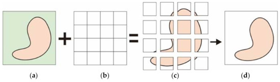
Figure 1.
Basic principle of filling an open hole using the Han method; (a) original closed hole; (b) partitioning grid; (c) open holes generated by partitioning; (d) open hole aggregation.
Step 2: A topographical surface is constructed in each block using the global optimal triangulation algorithm [18] based on the point clouds in the grid, with the various partitioning cells as processing units. During this process, the boundary line not involved in network construction is utilized as the range line for triangulation-based reconstruction.
Step 3: Surface reconstruction is completed in each partitioning cell in turn.
Step 4: Through the combination of the triangulated surfaces obtained for the various grid units based on the octree index, the open holes formed by the partitioning grids are reaggregated into closed holes, as shown in Figure 1d.
Step 5: The existence of holes in the partitioning grid is identified using a half-edge data structure. If holes exist, the fast and robust minimum area method [10] is used to retriangulate and subdivide the closed holes to achieve hole filling.
2.2. Limitations of the Existing Method
In the existing method of Han et al. [17], open holes are first transformed into closed holes through surface aggregation, and then, a mature algorithm for filling closed holes is used to solve the problem of hole filling. However, the following three limitations of the work of Han et al. [17] can be found:
(i) Open holes can be transformed into closed holes for filling after surface aggregation. However, the amount of data to be processed also increases. Specifically, the millions of triangular facets in a single block might expand to tens or hundreds of millions, leading to a significant increase in time and memory consumption. In rare cases, the computer may crash, resulting in failure to repair the holes.
(ii) Open holes may have various shapes. If the open holes are located completely within the reconstruction area and adjacent to each other, then they can be readily combined into closed holes through surface fusion. However, if the open holes are isolated at the edges of the reconstruction area, they cannot be converted into closed holes via surface fusion using existing methods.
(iii) The spatial areas spanned by the closed holes formed through surface aggregation vary. For holes with small areas, simple edge boundaries, and clear topological relations, the existing method has a satisfactory filling effect. However, for holes with large areas and boundaries and complex shapes, the surface characteristics cannot be expressed well by the surfaces generated via the existing method, reducing the quality of hole filling.
3. Methodology
A parallel method for open hole filling in large-scale 3D automatic modeling is proposed for the fast filling of open holes in oblique photography. In contrast to the existing method, surface aggregation is not performed in the proposed method. Instead, various block units are repaired independently, as each partitioning cell is considered a basic unit for the repair of open holes. This approach improves the calculation efficiency, overcoming limitation (i) of the existing method, and increases the types of open holes that can be processed without considering whether closed holes are formed with adjacent grids, thereby addressing limitation (ii) of the existing method. Furthermore, hierarchical relationships between open holes are established in this paper to enable hole repair considering the local information in the grid and the global shape formed between grid cells to ensure the repair accuracy, thereby addressing limitation (iii) of the existing method.
The newly proposed method consists of the following four key steps: (i) Identification and classification of open holes: Open holes are identified in accordance with a half-edge data structure and classified into two major categories and four types based on their shapes and location characteristics. (ii) Calculation of hierarchical relationships between open holes: A grid index is first established for the partitioning grid, and the hierarchical relations between open holes are calculated in accordance with the adjacency relationships between grid cells. (iii) Layer-by-layer propagation filling of open holes: Closure processing is performed in each partitioning cell based on the principle of topological closure, and height projection transformation is performed to complete the layer-by-layer repair of open holes. (iv) Smoothing processing of adjacent holes: The common boundaries between two adjacent partitioning cells are smoothed in conformity with the Laplacian algorithm to achieve natural transitions between triangulation results. The flowchart of our algorithm is shown in Figure 2.
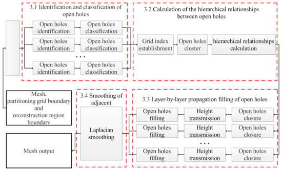
Figure 2.
Flowchart of a parallel method for open hole filling.
3.1. Identification and Classification of Open Holes
The identification of open holes is the first step in the filling process. In this paper, open holes are identified using a half-edge data structure, as described in the existing literature [19]. Specifically, adjacent triangles associated with a certain edge are identified from the triangular facets organized inside the half-edge data structure, as shown in Figure 3a. The two opposite halves h0,1 and h0,2 at edge e0,1 indicate that it is associated with two triangles; if an edge is associated with only one triangle, it is defined as a boundary edge. The boundary edges are tracked along a certain fixed direction (clockwise or counterclockwise); if the loop formed in this way includes a grid boundary, the hole is an open hole, as shown in Figure 3b.
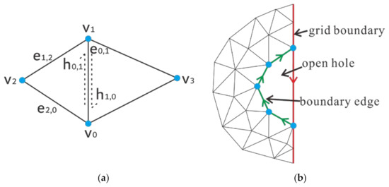
Figure 3.
Preliminaries: (a) a half-edge data structure; (b) a triangular mesh with an open hole.
Based on the positions of the open holes in the reconstruction area, the open holes are first classified into two categories: Type I, internal boundary holes, for which the grid boundary contained in the loop is not also a boundary of the reconstruction area, as shown in Figure 4a, and Type II, external boundary holes, for which the grid boundary contained in the loop is a boundary of the reconstruction area, as shown in Figure 4b.
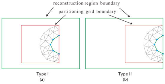
Figure 4.
Initial classification of open holes: (a) internal open holes; (b) external open holes.
The open holes are then further divided into four types according to their morphological characteristics:
Type A: Hollow type: There are no triangular surfaces in the partitioning cell; that is, the whole partitioning cell is an open hole, as shown in Figure 5a.
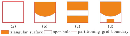
Figure 5.
Fine classification of open holes: (a) type A; (b) type B; (c) type C; (d) type D.
Type B: Semi-enclosed type: The open hole is located on one side of the partitioning cell, while the other side is an original triangular surface, as shown in Figure 5b.
Type C: Crossing type: The open hole is located in the middle of the partitioning cell, with both sides being original triangular surfaces, as shown in Figure 5c.
Type D: Island type: The open hole is located in the middle of the partitioning cell, both sides are original triangular surfaces, and one (or both) of the triangular surfaces is related to one or two segment(s) of the cell boundary, as shown in Figure 5d.
Other types of open holes can be obtained through simple deformation of these four basic types; hence, they are not discussed in detail here.
3.2. Calculation of the Hierarchical Relationships between Open Holes
Each partitioning cell is regarded as a basic unit for the repair of open holes. To ensure the repair quality, hierarchical relationships are established between open holes. First, a grid index is established to organize all partitioning cells. If the partitioning cells in which two open holes are located are adjacent to each other with a common grid boundary, they are clustered and labeled but not aggregated. The above process is iteratively performed until all open holes have participated in the calculation to achieve the clustering of every open hole. Second, the hierarchical division of the open holes in each cluster is performed in accordance with the following provisions. (i) The open holes located at the outermost edge of the cluster are holes in the first layer, which can be defined by identifying the boundary edges in the initial triangulation; that is, open holes with boundary edges are located in the first layer. (ii) Open holes sharing grid boundaries with holes in the first layer are holes in the second layer. (iii) By parity of reasoning, holes in the nth layer are identified so as to establish all hierarchical relationships between open holes. As an example, in Figure 6, the hierarchical relationships of the open holes in Figure 6a are illustrated in Figure 6b.
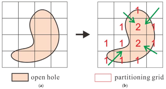
Figure 6.
Calculation of hierarchical relationships: (a) original partitioning grid and open holes; (b) hierarchical relationship calculation for the open holes.
3.3. Layer-by-Layer Propagation Filling of Open Holes
Based on the hierarchical relationships between the open holes, the holes are repaired layer by layer starting from the outermost holes (in the first layer) and proceeding to the innermost ones. Two critical problems arising during the repair process should be highlighted: (i) how to convert open holes into closed holes, i.e., implementing topological closure at boundaries, and (ii) how to reasonably fit the surfaces of holes in the grid, i.e., assigning appropriate heights to network-constructing points near the grid boundaries. To address these problems, a general topological closure algorithm is constructed to perform closure processing on various types of open holes, and layer-by-layer repair of open holes is accomplished through height projection transformation.
The boundary of any hole is first divided into the surface boundary and the grid boundary. The former is the boundary edge of the original triangular surface, while the latter is the boundary edge of the partitioning cell. Apparently, the grid boundary part of an open hole is not topologically closed with the surface boundary at the joint. In this case, the open hole cannot be converted into a closed hole for repair. Hence, accomplishing topological closure of open holes is a prerequisite for achieving conversion from open holes to closed holes.
Based on an analysis of the boundary characteristics of the four open hole types, the topological closure situation can be summarized into the following three cases: (1) The start and end points of the surface boundary edge are located on opposite sides of the grid boundary. In this case, a buffer zone is constructed on both sides of the grid boundary, with the distances between the start and end points and the grid boundary as the constraints. A topologically closed triangulation can be formed by selecting network-constructing points from the boundary of the buffer zone, as shown in Figure 7a. (2) A point on the surface boundary edge is located on the grid boundary, and the two boundary edge points adjacent to this point are located on opposite sides of the grid boundary. Similar to Case 1, a buffer zone is constructed on both sides of the grid boundary, with the distances between the adjacent points and the grid boundary as the constraints. Again, a topologically closed triangulation can be formed by selecting network-constructing points from the boundary of the buffer zone, as shown in Figure 7b. (3) A point on the surface boundary edge is located on the grid boundary, and both boundary edge points adjacent to this point are located inside the grid boundary. On this basis, a buffer zone is constructed outside the grid boundary, using the average distance of both adjacent boundary edge points. Then, a topologically closed triangulation can once again be formed by selecting network-constructing points from the boundary of the buffer zone, as shown in Figure 7c.
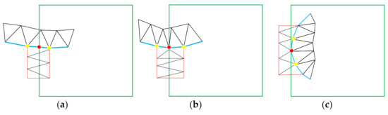
Figure 7.
Topologically closed triangulation: (a) case 1; (b) case 2; (c) case 3.
To ensure the accuracy of the hole fitting surface in a partitioning cell, appropriate height values should be assigned to network-constructing points near the grid boundary. For this purpose, height projection transformation is performed in this paper. First, the target boundary point is projected on the grid boundary to obtain the projection point as a new point on the grid boundary. This ensures that the new triangular facet will have a compactness similar to that of the original triangular facet, as shown in Figure 8a. Next, the boundary triangular facets associated with each boundary point are captured to calculate the average value of their centroid heights. Finally, each new point is assigned the average height associated with the corresponding boundary point, as shown in Figure 8b. Moreover, the four corner points of the partitioning cell are regarded as split points to partition the grid boundary into four parts to enhance the accuracy of height assignment. On this basis, the above algorithm is used to obtain each new point and its corresponding height on each part of the boundary.
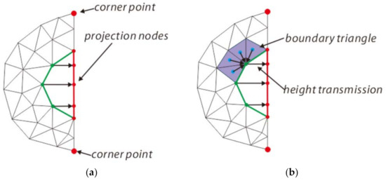
Figure 8.
Grid boundary assignment: (a) point projection; (b) height transmission.
In the process of repairing open holes, the heights of the grid boundaries of the various partitioning cells in the first layer are assigned before transmitting the height information to the second layer. Then, the propagation process in the second layer is the same as that within a partitioning cell. Based on the above algorithm, open holes can be converted into topologically closed holes, and suitable points for triangulation are provided for the grid boundaries. Thus, the surfaces in the resulting closed holes can be fitted with the minimum area method [10] to achieve hole filling. The necessary tasks include hole triangulation, mesh refinement, mesh adjustment, and mesh fairing.
Mesh Adjustment: For the newly added patching mesh, an adjustment sequence is applied that proceeds from the outside to the inside, and an inner ring is extracted based on the connection relationships of the newly added patching mesh, as shown in Figure 9a. The outermost ring is adjusted first, and then the second-to-outermost ring is adjusted. The adjustment method used is the reciprocal-distance-weighted averaging algorithm, which ensures that the farther away a position is from a newly added point, the lower the impact of the newly added point on that position. First, we calculate the first-order neighbors (blue points) and second-order neighbors (green points) of the newly added outermost points, as shown in Figure 9b; second, we calculate the weight of each neighboring point; and finally, we use the weighted averaging algorithm to adjust the positions layer by layer from the outside to the inside. For illustration, in Figure 9c, the dark gray points are adjusted first, and then the light gray points are adjusted. The adjustment function is as follows:
where and is an adjacent point of the newly added point v, as indicated by the yellow arrows in Figure 9c above.
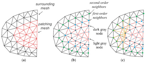
Figure 9.
Mesh Adjustment: (a) mesh refinement; (b) adjacent point extraction; (c) mesh adjustment.
Mesh Fairing: The newly added patching mesh needs to be smoothed. Curvature-based global smoothing can ensure that the new grid cells better maintain the approximate original shape of the model. The most popular existing mesh smoothing method uses the weighted center of gravity of the neighborhood of each point as the position of the corresponding new vertex; this is defined as the weighted umbrella operator and involves solving the Laplacian matrix:
where is a neighboring point and is the weight value of the corresponding edge.
The difference between curvature-based smoothing and the above Laplacian smoothing method is that curvature-based smoothing moves vertex v along its normal vector, while general Laplacian smoothing moves vertex v to a similar center-of-gravity position. After derivation, by selecting the appropriate Laplacian weights, it can be found that smoothing based on curvature and Laplacian smoothing achieve the same effect [20]. We define
The umbrella operator can be applied recursively to obtain a second-order weighted umbrella operator:
For manifold surfaces, if measures the deviation of a vertex from a taut surface bounded by its neighbors, then implies that the deviation from tautness at vertex v is equal to the average deviation from tautness of its neighbors [21].
3.4. Smoothing of Adjacent Holes
After layer-by-layer processing, all open holes inside each partitioning cell have been repaired. However, a height difference can often be found at the “shared” boundary of two adjacent partitioning cells in the same layer due to layered processing, as shown in Figure 10. Therefore, the “shared” boundaries of adjacent holes in the same layer should be smoothed.
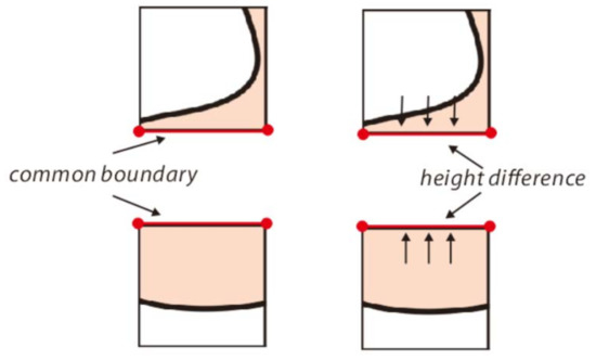
Figure 10.
Height difference at a common boundary.
Laplacian smoothing, with its features of simple calculation and a short calculation time, is extensively applied in surface smoothing [22] and facilitates a uniform grid based on maintaining the local geometric details of the surface. For this reason, the height of a shared boundary is smoothed using the Laplace smoothing method in accordance with the principle of assigning the height of each point to be the average elevation of the points within a certain buffer range.
For each point to be repaired, let p be the initial height, and let its updated height be :
where is smooth and sparse, 0 < < 1, and is defined as follows:
where is the th point in the neighborhood of the point to be repaired and m is the number of neighborhood points.
4. Experiments and Analyses
4.1. Experimental Data and Running Environment
The method proposed in this paper was embedded into the NewMap-IMS software, which is a reality modeling software independently developed by the authors at the Chinese Academy of Surveying and Mapping. A 5.2 km × 7.8 km built-up urban area in Shandong Province, China, was chosen as the experimental area. A 5-lens (1 vertical-view lens + 4 side-view lenses) UltraCam Osprey Prima (UCOp) camera was used in 29 flights to collect 11,795 images, totaling 2.08 TB of data. The corresponding reconstruction area is approximately 28 km2. The reconstruction area is divided into 449 subareas with a grid size of 250 m × 250 m, as shown in Figure 11. The operating environment is a standard personal computer equipped with the Windows 10 64-bit operating system, an Intel Xeon(R) E3-1535M CPU with a dominant frequency of 3.10 GHz, and 64 GB of memory. The effectiveness and superiority of the proposed method are validated by comparatively analyzing the proposed method and the method proposed by Han et al. [17]. The experiments are composed of three parts: a comparative analysis of the filling success rate, a comparative analysis of the filling efficiency, and a comparative analysis of the filling accuracy.
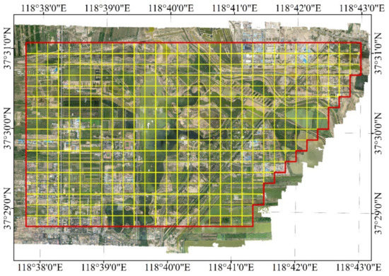
Figure 11.
Experimental area and reconstruction area.
4.2. Comparative Analysis of Filling Success Rate
- Comparison of the filling success rates in a local experimental area
An area covering 2 km2 in the middle of the reconstruction area is selected for a comparative experiment on the success rate of filling open holes. The areas of the open holes in the selected area range from 1242.99 m2 to 13,703.97 m2. The distributions and repair statistics of type I and type II open holes are shown in Table 1 and Table 2, respectively.

Table 1.
Distribution and repair statistics of closed holes and type I open holes.
Table 2.
Distribution and repair statistics of type II open holes.
According to Table 1, there are 16 closed holes located inside partitioning cells. Since the minimum area method is used for the hole filling process in the proposed method as well as in the Han method, both methods can repair closed holes at a repair rate of 100%. For type I open holes, most of the holes (17) are of type B and there are no type C holes in the selected area. Overall, the success rates of hole filling using the Han method and the proposed method are 50% and 100%, respectively, indicating that the proposed method has a markedly higher filling success rate. The difference between the two methods is most evident in the processing of type A and type B holes. Relative to the actual data, three type A boundary holes and eight type B boundary holes are not repaired by the Han method and constitute a closed hole with a large area, which leads to repair failure.
As shown in Table 2, there are only 2 Type II open holes in this local experimental area, indicating that the number of Type II open holes is significantly lower than that of Type I open holes. Type II open holes cannot be repaired at all using the Han method since they cannot be aggregated with adjacent holes to form closed holes. In contrast, these open holes can be filled by the method proposed in this paper, showing that the proposed method is superior in terms of applicability.
In order to better illustrate the reliability of the method proposed in this paper, we artificially dig holes in the reconstructed data of the selected area to increase the number of various types. For closed holes, the number is increased from 16 to 20; For Type I open holes, Type-A holes are increased from 4 to 5, Type-B holes are increased from 17 to 20, Type-C holes are increased from 0 to 4, and Type-D holes are increased from 1 to 4. For Type II open holes, the number of holes has not been changed because the Han method cannot be repaired. The distributions and repair statistics of Type I open holes are shown in Table 3.
Table 3.
Distribution and repair statistics of closed holes and type I open holes.
As shown in Table 3, for closed holes, both methods can repair closed holes at a repair rate of 100%. For Type I open holes, the success rate of Han method is improved, mainly because the newly added holes are not located in the large area of previous failures.
- 2.
- Comparison of the filling success rates in the global experimental area
A comparison of the success rates of open hole filling is also performed for the global reconstruction area, covering 28 km2 of the entire experimental area. The distributions and repair statistics of closed holes and Type I and Type II open holes are presented in Table 4 and Table 5.
Table 4.
Distribution and repair statistics of closed holes and type I open holes.
Table 5.
Distribution and repair statistics of type II open holes.
As shown in Table 4 and Table 5, the global experimental area contains 56 closed holes, 67 type I open holes, and 6 type II open holes. However, the Han method cannot handle these holes due to the large size of the experimental area serving as input data. In contrast, the proposed method can successfully fill all holes by processing each partitioning cell individually.
4.3. Comparative Analysis of Filling Efficiency
In the reconstruction area, six groups of areas covering 0.5 km2, 1 km2, 1.5 km2, 2 km2, 2.5 km2, and 28 km2 are selected for open hole filling experiments. The time and memory consumed using the Han method and the proposed method to fill the holes in these areas are determined for comparative analysis. The time measurement starts at the completion of triangulation reconstruction in the grid and ends at the completion of filling in open holes, including the identification, filling, and smoothing processes.
- Comparison of hole filling time consumption
The time consumption statistics of the two methods for hole filling in experimental areas of varying sizes are shown in Table 6, and a corresponding bar graph is presented in Figure 12.
Table 6.
Comparison of the time consumed using the two methods for hole filling in different experimental areas.
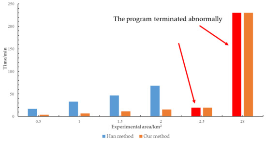
Figure 12.
Bar graph for the time consumption comparison.
As illustrated in Table 6 and Figure 12, (i) with increasing experimental area, the time consumption of both methods increases, but overall, the time consumption of the method proposed in this paper is lower than that of the Han method. (ii) The Han method is applicable only for hole filling within a small area (≤2 km2). When the experimental area is too large (>2 km2), the use of the Han method leads to the program terminating abnormally because of the excessive amount of data to be processed. (iii) Within the repairable scope (≤2 km2), the time consumed busing the Han method is approximately 4‒5 times greater than that consumed by the proposed method.
- 2.
- Comparison of memory consumption for hole filling
The memory consumption statistics of the two methods for hole filling in experimental areas of varying sizes are shown in Table 7, and a corresponding bar graph is presented in Figure 13.
Table 7.
Comparison of the memory consumed using the two methods for hole filling in different experimental areas.
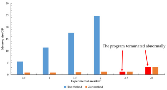
Figure 13.
Bar graph for the memory consumption comparison.
As illustrated in Table 7 and Figure 13, (i) similar to the time consumption, the memory consumption of both methods increases with increasing experimental area. However, the memory consumption of the proposed method increases only slowly, whereas the Han method incurs significantly higher memory consumption that increases relatively rapidly. (ii) When the experimental area is large (>2 km2), the use of the Han method in a single-computer environment leads to computer crashes due to memory limitations, resulting in failure to complete hole filling. (iii) The memory consumption of the Han method is approximately 7–21 times greater than that of the proposed method within the repairable scope.
4.4. Comparative Analysis of Filling Accuracy
To verify the filling results and accuracy of the proposed method, a closed hole and an unclosed hole, covering a total area of 76,112.5 m2, are artificially created in a complete area of the triangulation surface in the experimental area. Based on this, the experimental area is divided into four parts, dividing the closed hole into four internal boundary holes and the unclosed hole into two external boundary holes, as shown in Figure 14.
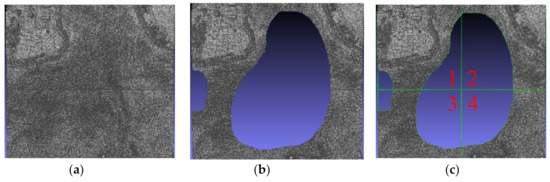
Figure 14.
(a) Original triangular surface; (b) closed and unclosed holes created manually; (c) six open holes created by partitioning.
- Comparison of Hole Filling Results
The filling results of the Han method and the proposed method are qualitatively evaluated, as shown in Figure 15 and Figure 16, respectively. In the Han method, after the open holes are aggregated, the internal boundary holes are transformed into an internal closed hole, which can be repaired; however, the external boundary holes still form a boundary hole and cannot be repaired, as shown in Figure 15a‒c. In the proposed method, after the open holes are closed, the inner and outer boundary holes are both transformed into internal holes, which can be repaired, as shown in Figure 16a‒c. In addition, in the repair results at the boundary of the closed hole, the boundary line of the hole repaired using the Han method is clearly visible, while the surface repaired using the method proposed in this paper transitions more naturally, as shown in Figure 15c and Figure 16c.
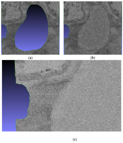
Figure 15.
Hole filling results obtained via the Han algorithm: (a) open hole aggregation; (b) hole filling; (c) hole filling details.
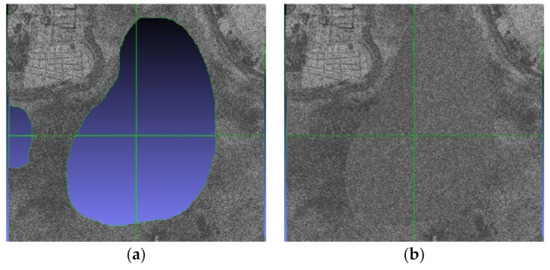
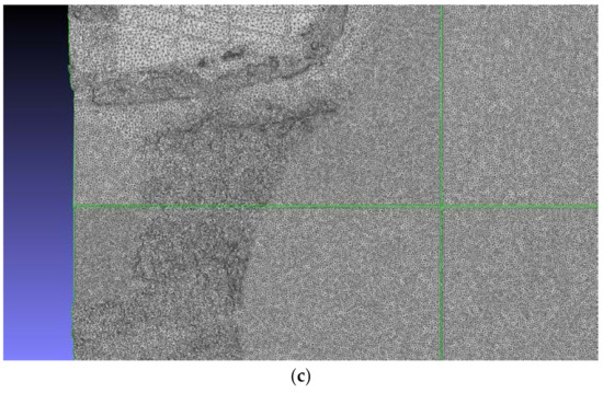
Figure 16.
Hole filling results obtained via the method proposed in this article: (a) open hole closure; (b) hole filling; (c) hole filling details.
- 2.
- Comparison of Hole Filling Accuracy
The filling accuracy is evaluated in terms of the difference between the height values of a point in the filled triangulation network and the corresponding point in the original triangulation network. In this experiment, the height of the surface over the whole closed hole ranges from 3.96 m to 5.98 m, presenting a height difference of 2.02 m. Thirty-four uniformly distributed points are selected from the closed hole area, and the differences between the heights obtained with the above two methods and the corresponding original heights are determined. The results are presented in Figure 17.
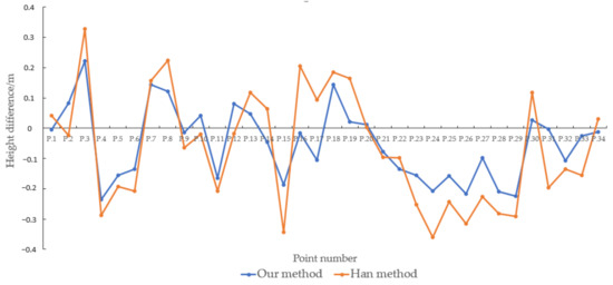
Figure 17.
Comparative analysis of the filling accuracy.
According to Figure 17, the average difference between the elevation values of the triangular mesh repaired via the Han method and the original triangular mesh is 16 cm, and the maximum error is 36 cm. In comparison, the average difference between the elevation values of the triangular mesh repaired via the proposed method and the original triangular mesh is 10 cm, and the maximum error is 23 cm. Moreover, the standard deviations of the height differences obtained with the Han method and the proposed method are 18 cm and 11 cm, respectively, indicating that the points generated via the proposed method are characterized by high overall elevation accuracy and minor errors. The closer a point is to the center of the hole, the greater the height difference with respect to the original point. This is directly associated with the process of triangulation-based hole filling and indicates that the filling accuracy decreases with increasing hole size. Hence, more research on further accuracy improvement will be required in the future.
5. Conclusions
Open hole filling is of great significance for improving the quality of 3D reconstruction for large-scale 3D automatic modeling based on oblique photography. A common solution at present is manual repair, and few automated methods have been proposed. A natural automatic filling method involves reaggregating open holes into closed holes and then filling the resulting holes with mature closed hole filling methods used in industrial design, medical imaging, and the study of cultural relics. However, this method encounters various problems such as long calculation times, high memory consumption, unsuccessful hole filling, and low fitting accuracy of the hole surface. Hence, this paper proposes a parallel method for open hole filling in large-scale 3D automatic modeling. Open holes are filled by taking each individual partitioning cell as a basic filling unit, and the applicability is strengthened through the assurance of higher repair accuracy in addition to improving the efficiency of hole filling. Experiments have been conducted using real survey data to evaluate the rationality and effectiveness of the proposed method, and the following conclusions can be drawn.
- Concerning the filling success rate, for closed holes, which are commonly encountered in large-scale 3D automatic modeling, the proposed method is consistent with the state-of-the-art Han method. Additionally, the proposed approach has a 12.4% higher success rate for filling type I open holes than the Han method and successfully compensates for the limitations of the existing method in the filling of type II open holes.
- In terms of the efficiency of hole filling, when implemented on a standard personal computer, the Han method is applicable only for hole filling in a small area (≤2 km2). When the experimental area is large (>2 km2), the use of the Han method leads to computer crashes because of the excessive amount of data to be processed. Moreover, even within the repairable scope, the time consumption of the Han method is approximately 4–5 times greater than that of the proposed method, and its memory consumption is approximately 7–21 times greater.
- Regarding the repair accuracy, the proposed method exhibits high height accuracy and minor errors, with the average and standard deviation of the height differences being 37.5% and 38.9% lower than those of the Han method, respectively.
In our future research, the following insufficiencies of the proposed method will be extensively studied. (1) When the length of the grid boundary accounts for a large proportion of the overall boundary length for an open hole, if the individual partitioning cell is treated as the elementary repair unit, only a small number of points constructed for topological closure are determined via the proposed method, resulting in a decline in the height accuracy. Future research should address how to identify this situation on the basis of the boundary length proportion and calculate the point position and height considering the hole boundary information contained in the adjacent partitioning cell. (2) How to reasonably fit the reconstruction surface is a difficult issue for holes with large areas. The proposed method is designed on the basis of partitioning large-scale holes into grid cells for reconstruction. However, its reconstruction accuracy should be further improved. More reasonable surface fitting methods, such as the least squares method, the radial basis function (RBF) implicit surface algorithm, Newton interpolation, and other algorithms, need to be introduced to improve the accuracy of reconstruction.
Author Contributions
Conceptualization, F.W. and H.Z.; methodology, F.W., Z.L., P.W. and H.Z.; software, F.W. and Z.L.; validation, F.W., Z.L. and P.W.; writing—original draft preparation, H.Z., F.W. and P.W.; supervision, H.Z. All authors have read and agreed to the published version of the manuscript.
Funding
This work was supported by the auspices of the National Natural Science Foundation of China (Grant No. 41971339), National Key Research and Development Project of China (Grant Nos. 2018YFB2100704, 2018YFC1407605), Basal Research Fund of CASM (Grant Nos. AR2107, AR2108, AR2120) and SDUST Research Fund (Grant No. 2019TDJH103).
Institutional Review Board Statement
Not applicable.
Informed Consent Statement
Not applicable.
Data Availability Statement
Data available on request due to privacy restrictions.
Conflicts of Interest
The authors declare no conflict of interest.
References
- Bendels, G.H.; Schnabel, R.; Klein, R. Detecting holes in point set surfaces. J. WSCG 2006, 14, 89–96. [Google Scholar]
- Chalmovianský, P.; Jüttler, B. Filling Holes in Point Clouds. In Mathematics of Surfaces; Springer: Berlin/Heidelberg, Germany, 2003; pp. 196–212. [Google Scholar]
- Guo, X.; Xiao, J.; Wang, Y. A survey on algorithms of hole filling in 3D surface reconstruction. Vis. Comput. 2018, 34, 93–103. [Google Scholar] [CrossRef]
- Argudo, O.; Brunet, P.; Chica, A.; Vinacua, À. Biharmonic fields and mesh completion. Graph. Models 2015, 82, 137–148. [Google Scholar] [CrossRef] [Green Version]
- Davis, J.; Marschner, S.R.; Garr, M.; Levoy, M. Filling Holes in Complex Surfaces using Volumetric Diffusion. In Proceedings of the First International Symposium on 3D Data Processing Visualization and Transmission, Padua, Italy, 19–21 June 2002; pp. 428–441. [Google Scholar]
- Guo, T.-Q.; Li, J.-J.; Weng, J.-G.; Zhuang, Y.-T. Filling Holes in Complex Surfaces using Oriented Voxel Diffusion. In Proceedings of the 2006 International Conference on Machine Learning and Cybernetics, Dalian, China, 13–16 August 2006; pp. 4370–4375. [Google Scholar]
- Ju, T. Robust repair of polygonal models. ACM Trans. Graph. 2004, 23, 888–895. [Google Scholar] [CrossRef] [Green Version]
- Altantsetseg, E.; Khorloo, O.; Matsuyama, K.; Konno, K. Complex Hole-Filling Algorithm for 3D Models. In Proceedings of the Computer Graphics International Conference, Yokohama, Japan, 27–30 June 2017; pp. 1–6. [Google Scholar]
- Jun, Y. A piecewise hole filling algorithm in reverse engineering. Comput. Aided Des. 2005, 37, 263–270. [Google Scholar] [CrossRef]
- Kobbelt, L.; Schröder, P.; Hoppe, H. Filling Holes in Meshes. In Proceedings of the Eurographics Symposium on Geometry Processing, Aachen, Germany, 23–25 June 2003; Available online: https://dl.acm.org/doi/proceedings/10.5555/882370 (accessed on 16 August 2021).
- Wu, X.; Chen, W. A Scattered Point Set Hole-Filling Method Based on Boundary Extension and Convergence. In Proceedings of the 11th World Congress on Intelligent Control and Automation, Shenyang, China, 29 June–4 July 2014; pp. 5329–5334. [Google Scholar]
- Huang, H.; Zhou, L.; Chen, X.; Gong, Z. SMART robotic system for 3D profile turbine vane airfoil repair. Int. J. Adv. Manuf. Technol. 2003, 21, 275–283. [Google Scholar] [CrossRef]
- Li, E.; Zhang, X.; Chen, Y. Sampling and Surface Reconstruction of Large Scale Point Cloud. In Proceedings of the 13th ACM SIGGRAPH International Conference on Virtual-Reality Continuum and its Applications in Industry, Shenzhen, China, 30 November–2 December 2014; pp. 35–41. [Google Scholar]
- Marton, Z.C.; Rusu, R.B.; Beetz, M. On Fast Surface Reconstruction Methods for Large and Noisy Point Clouds. In Proceedings of the 2009 IEEE International Conference on Robotics and Automation, Kobe, Japan, 12–17 May 2009; pp. 3218–3223. [Google Scholar]
- Qi, Z.; ShuZhen, L.; Jialu, B.; Jiarang, Z. Opening-hole repairing in point cloud based on improved curve contraction flows. Laser Optoelectron. Prog. Las. Optoelect. Prog. 2018, 119–125. [Google Scholar] [CrossRef]
- Mostegel, C.; Prettenthaler, R.; Fraundorfer, F.; Bischof, H. Scalable Surface Reconstruction from Point Clouds with Extreme Scale and Density Diversity. In Proceedings of the IEEE Conference on Computer Vision and Pattern Recognition, Honolulu, HI, USA, 21–26 July 2017; pp. 904–913. [Google Scholar]
- Han, J.; Shen, S. Scalable point cloud meshing for image-based large-scale 3D modeling. Vis. Comput. Ind. Biomed. Art 2019, 2, 1–9. [Google Scholar] [CrossRef] [PubMed]
- Vu, H.-H.; Labatut, P.; Pons, J.-P.; Keriven, R. High accuracy and visibility-consistent dense multiview stereo. IEEE Trans. Pattern Anal. Mach. Intell. 2011, 34, 889–901. [Google Scholar] [CrossRef] [PubMed]
- Feng, C.; Liang, J.; Ren, M.; Qiao, G.; Lu, W.; Liu, S. A fast hole-filling method for triangular mesh in additive repair. Appl. Sci. 2020, 10, 969. [Google Scholar] [CrossRef] [Green Version]
- Desbrun, M.; Meyer, M.; Schröder, P.; Barr, A.H. Implicit Fairing of Irregular Meshes using Diffusion and Curvature Flow. In Proceedings of the 26th Annual Conference on Computer Graphics and Interactive Techniques, Los Angeles, CA, USA, 8–13 August 1999; pp. 317–324. [Google Scholar]
- Liepa, P. Filling Holes in Meshes. In Proceedings of the 2003 Eurographics/ACM SIGGRAPH Symposium on Geometry Processing, Aachen, Germany, 23–25 June 2003; pp. 200–206. Available online: http://diglib.eg.org/handle/10.2312/SGP.SGP03.200-206 (accessed on 16 August 2021).
- Liao, T.; Li, X.; Xu, G.; Zhang, Y.J. Secondary Laplace operator and generalized Giaquinta–Hildebrandt operator with applications on surface segmentation and smoothing. Comput. Aided Des. 2016, 70, 56–66. [Google Scholar] [CrossRef]
Publisher’s Note: MDPI stays neutral with regard to jurisdictional claims in published maps and institutional affiliations. |
© 2021 by the authors. Licensee MDPI, Basel, Switzerland. This article is an open access article distributed under the terms and conditions of the Creative Commons Attribution (CC BY) license (https://creativecommons.org/licenses/by/4.0/).