Adaptive Network Detector for Radar Target in Changing Scenes

Abstract

Data-driven deep learning has been well applied in radar target detection. However, the performance of the detection network is severely degraded when the detection scene changes, since the trained network with the data from one scene is not suitable for another scene with different data distribution. In order to address this problem, an adaptive network detector combined with scene classification is proposed in this paper. Aiming at maximizing the posterior probability of the feature vectors, the scene classification network is arranged to control the output ratio of a group of detection sub-networks. Due to the uncertainty of classification error rate in traditional machine learning, the classifier with a controllable false alarm rate is constructed. In addition, a new network training strategy, which freezes the parameters of the scene classification network and selectively fine-tunes the parameters of detection sub-networks, is proposed for the adaptive network structure. Comprehensive experiments are carried out to demonstrate that the proposed method guarantees a high detection probability when the detection scene changes. Compared with some classical detectors, the adaptive network detector shows better performance.

1. Introduction

As the most basic task of radar signal processing, radar target detection is widely used in military and civil aviation activities. In traditional detection methods, statistical inference based on probability distribution is used to distinguish the target of interest from clutter [1,2,3]. However, due to the complexity of clutter distribution, various methods can not match the clutter and target characteristics accurately, resulting in performance degradation.

In this case, the different features of clutter and target are usually extracted to realize a binary classification, which is called feature detection technology. These features usually include the radar echo amplitude, doppler spectrum, time-frequency map, polarization information, and other aspects [4,5,6,7,8]. For example, according to the fractal feature of the sea clutter and the target, some detectors are proposed to gain a high performance [9,10,11]. Using three separable features from time domain and frequency domain, the target detection is realized [12,13]. Based on the three polarization features, a three-dimensional feature detector is proposed to detect the small floating targets on the sea [14].

As the further development of feature detection technology, the method of using deep learning to detect targets in high-dimensional feature space has been proposed, which greatly improves the detection performance [15,16,17,18,19]. The advantage of this method is that it automatically selects and fully extracts features with greater differences between the clutter and the target, and automatically obtains detection results. Applications of deep networks to target detection have been in practice for some years [20,21,22,23]. The network detection methods can be divided into two categories, one is based on signal prediction, and the other is based on feature classification [24,25]. The former uses the threshold of clutter prediction error to get the detection judgement, and the latter uses the different features between the clutter and the target for binary detection. In the literatures, the integrated output of Radial Basis Function Neural Network (RBFNN) and General Regression Neural Network (GRNN) is used to predict sea clutter and detect small targets floating on the sea surface [26]. A long-short-term memory network (LSTM) sequence prediction is compared with subsequent signals to achieve target detection [27]. The application of Generative Adversarial Networks (GAN) with a pre-processing stage based on range-Doppler analysis is presented to perform clutter suppression and target detection [28]. A deep symmetric positive definite (SPD) matrix learning network is designed to detect the target signal [29]. Several researchers [30,31,32] also suggest the use of Convolutional Neural Network (CNN) to classify the time-frequency spectrum for target detection.

However, as the target detection method based on deep learning is a data-driven adaptive technology, it is limited by the quality of the dataset. When the detection scene changes, such as the detection area is located between different characteristic areas, ultimate performance degradation occurs in target detection. As the change of detection scene means the change of data distribution, the network trained with one scene is not suitable for another scene. Typical detection scenes include the boundary of the ground and the sea, the edge of the rainfall area and so on [33,34,35].

In order to address above problem, an adaptive network detector combined with scene classification is proposed in this paper. The scene classification network is designed to recognize the background clutter distribution, which represents a priori information about detection scenes. Aiming at maximizing the posterior probability of feature vectors, the output probability of the scene classification network is used to control the output ratio of a group of detection sub-networks. In addition, the detection sub-networks are integrated to tackle performance degradation. Finally, a constant false alarm detection output module is constructed to control the false alarm rate, which is an important index. In addition, a new network training strategy, which freezes the parameters of the scene classification network and selectively fine-tunes the parameters of detection sub-networks, is devised for the network structure. Accordingly, combining the target detection of each scenes, the proposed adaptive network detector can achieve data adaptation, complete the intelligent and integrated detection process, and adapt to the changing scenes.

2. Methods

The basic idea of the adaptive network detector is to use CNN extracting features of the input time-frequency maps for clutter and target classification. At the same time, considering the change in the detection scenes, a network structure is designed, which combines the scene classification network and the target detection network group. In addition, an optimization strategy of network training is also proposed to realize the data adaptation.

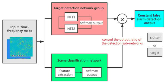
2.1. The Detector Framework

As shown in Figure 1, the border area of the ground and the sea is a typical example of changing scenes. When the aircraft target flies over the coastline, the clutter background characteristics are significantly different, and the performance of the network detection method is degraded. Based on this, the adaptive network detector is designed as follows.

Figure 1. Schematic diagram of the detection scene. It depicts the scene of an aircraft target flying over the land-sea border area. This scene is a typical example of changing scenes, and is the research scene set in the experiment of this paper.

Firstly, the adaptive network detector uses CNN extracting features of the input time-frequency maps for clutter and target classification. It is similar to putting time-frequency maps into a nonlinear system, which is capable of transforming the data space into a new feature space. Through the processing of the nonlinear system, as shown in Equation (1), the function of feature extraction is implemented.

$$f=f_{\mathrm{fc}}\left(f_{\mathrm{cov}}\left(\mathrm{image}\right)\right)$$

(1)

where $f_{\mathrm{fc}}$ is the fully connected operation, $f_{\mathrm{cov}}$ is the convolution operation, and $\mathrm{image}$ represents the input time-frequency map.

Accordingly, the distribution of the input in the new feature space ${\mathcal{S}}_{\theta }$ is evaluated. The specific feature vectors are referred to $\theta =[f_t,f_c]$, where $f_t$ is the target feature component and $f_c$ is the clutter feature component. Considering the changing scenes $D_1$ and $D_2$, the observation data x is denoted as $x\in D,D=D_1\cup D_2$. With the event $E=x\in D$, $E_1=x\in D_1$ and $E_2=x\in D_2$, the posterior probability of the feature vectors can be expressed as

$$p(\theta \mid E)=\frac{p(E\mid \theta )p\left(\theta \right)}{p\left(E\right)}$$

(2)

Assuming that the mapping of data $x\in D_1$ and $x\in D_2$ on the new feature space ${\mathcal{S}}_{\theta }$ is mutually exclusive, we derive the above formula as follows:

$$\begin{array}{cc}\hfill p(\theta \mid E)& =\frac{\left[p\right(E_1\mid \theta )+p(E_2\mid \theta \left)\right]p\left(\theta \right)}{p\left(E\right)}\hfill \\ \hfill & =\frac{p(E_1\mid \theta )p\left(\theta \right)}{p\left(E\right)}+\frac{p(E_2\mid \theta )p\left(\theta \right)}{p\left(E\right)}\hfill \\ \hfill & =\frac{p(\theta \mid E_1)p\left(E_1\right)}{p\left(E\right)}+\frac{p\left(\theta E_2\right)p\left(E_2\right)}{p\left(E\right)}\hfill \\ \hfill & =p(E_1\mid E)p(\theta \mid E_1)+p(E_2\mid E)p(\theta \mid E_2)\hfill \end{array}$$

(3)

The objective then becomes a matrix form as:

$$[p_{\mathrm{ft}},p_{\mathrm{fc}}]=[p_{\mathrm{E}1},p_{\mathrm{E}2}]·\left[\begin{array}{cc}{p}_{\mathrm{Elt}}& p_{\mathrm{Elc}}\\ p_{\mathrm{E}2\mathrm{t}}& p_{\mathrm{E}2\mathrm{c}}\end{array}\right]$$

(4)

where $[p_{\mathrm{ft}},p_{\mathrm{fc}}]$ is the ultimate probability that a sample data belongs to the target or the clutter. $p_{\mathrm{E}1}$ and $p_{\mathrm{E}2}$ are the probabilities of the event $E_1$ and $E_2$. $[p_{\mathrm{E}1\mathrm{t}},p_{\mathrm{E}1\mathrm{c}}]$ and $[p_{\mathrm{E}2\mathrm{t}},p_{\mathrm{E}2\mathrm{c}}]$ represent the outputs of NET1 and NET2 respectively.

From the Bayesian perspective, the detection decision requires minimum misclassification probability, i.e., maximum posterior probability. Thus, the parameter training process of deep networks meets the requirement.

Accordingly, the network structure proposed in this paper is conceived as shown in Figure 2. The output result of the whole network is the probability $[p_{\mathrm{ft}},p_{\mathrm{fc}}]$, which represents the ultimate probability that a sample data belongs to the target or the clutter. The scene classification network adopts Residual Network (ResNet) as a basic model, and the network output is the probability of the event $E_1$ and $E_2$, which refers to $[p_{\mathrm{E}1},p_{\mathrm{E}2}]$. The target detection sub-networks both use LeNet as the basic model, and the sub-networks are arranged parallelly as $\left[\begin{array}{cc}{p}_{\mathrm{E}1\mathrm{t}}\hfill & p_{\mathrm{E}1\mathrm{c}}\hfill \\ p_{\mathrm{E}2\mathrm{t}}\hfill & p_{\mathrm{E}2\mathrm{c}}\hfill \end{array}\right]$ in the target detection network group. Besides, the scene classification network and the target detection network group are connected by a multiplier.

Figure 2. Framework of the adaptive network detector.

Besides, the specific sub-network structure is shown in Figure 3. The scene classification network adopts Residual Network (ResNet) as a basic model. A skip connection is introduced, hence the information from the previous residual block flows into the next residual block without hindrance. It can better recognize the multi-type detection scenes. In addition, the target detection sub-networks both use LeNet as the basic model. It has less hierarchy and fewer parameters, which is enough to deal with simple data.

Figure 3. Network structure. (a) The structure of Scene classification network. (b) The structure of Target detection network.

Finally, a constant false alarm rate module is added to meet the detection requirements. The main idea is to control the sample prediction probability in the final classification stage. As the vector of the output layer is $[p_{\mathrm{ft}},p_{\mathrm{fc}}]$, where $p_{\mathrm{ft}}$ is the probability that the sample belongs to a target signal and $p_{\mathrm{fc}}$ is the probability that the sample belongs to a clutter signal, the threshold is set by the second component of the array to meet a controllable false alarm rate.

$$i=\lceil P_{\mathrm{fa}}·N_c\rceil$$

(5)

$$T=o_i$$

(6)

where $P_{\mathrm{fa}}$ is the false alarm rate to be controlled, $N_c$ is the number of clutter samples, and $\lceil \rceil$ represents rounding operation. o is the prediction probability set sorted by the second component, and T is the probability threshold for predicting the samples as clutter.

2.2. The Training Strategy

An optimization training strategy is also proposed for the network structure. With part of the dataset, the pre-trained scene classification network and the pre-trained target detection network are used to build the detector. In addition, all the dataset D is used to retrain the network detector, which makes the output results approach the true value on the entire dataset. Specifically, the parameters of the scene classification network are controlled to no longer being updated, and the parameters of the target detection network group are fine-tuned. The design is based on the consideration of the actual situation. The dataset collected by the radar is in the case of mixed scenes, and there are only accurate records of clutter and target, but no scene information.

3. Experimental Setup

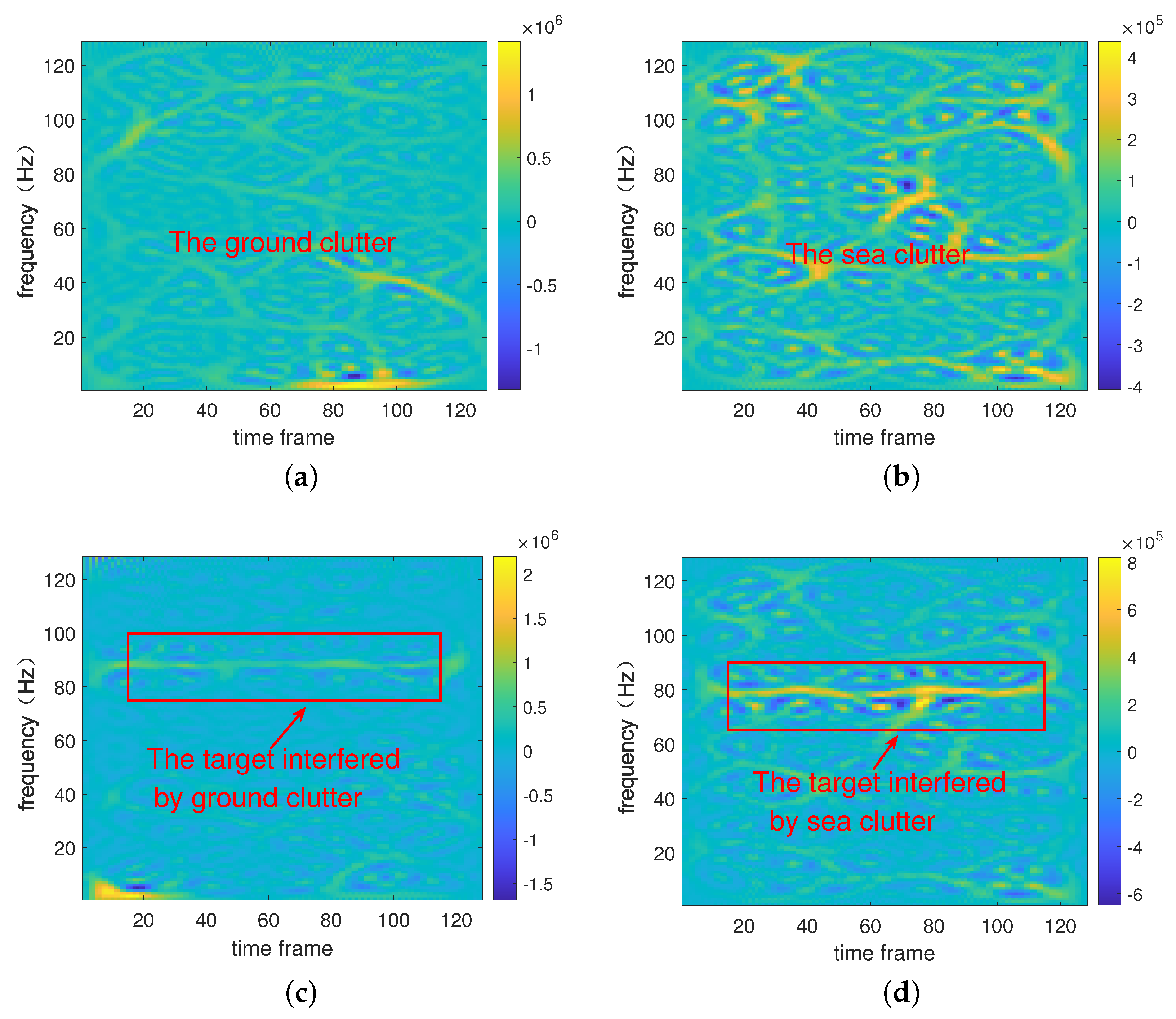
3.1. Experimental Dataset

The data used for model training and testing includes two categories: real clutter and simulated target-plus-clutter. The real clutter uses a dataset for detection and tracking of dim aircraft targets through radar echo sequences [36], and the data numbered 11 and 14 are selected for experiments. Among them, Data11 is the ground clutter data, and Data14 is the sea clutter data. Table 1 shows the main information of the dataset. In this paper, the experiment of mixing two kinds of data is used to simulate the changing of detection scenes.

Table 1. The main information of the dataset.

Index Item	Content
Measurement time and place	In Meixian, China from 2017 to 2019
Waveform	Linear Frequency Modulation(LFM)
Carrier frequency	35 GHz
Pulse repetition frequency(PRF)	32 kHz
Data format	A two-dimensional time-domain pulse sequence

As for the examples of target-plus-clutter, the selected real clutter vector is added to a target signal synthetically generated according to:

$$t\left(n\right)=\sqrt{SCR·P_c}·e^{j\varphi }·e^{j2\pi f_{d}n}$$

(7)

$$P_c=\frac{1}{l_c}\sum _{i=1}^{l_c}c\left(i\right)·c^{*}\left(i\right)$$

(8)

where the phase $\varphi$ is Uniform-distributed in $[0,2\pi )$ and the Doppler frequency $f_d$ is Uniform-distributed in $[0.29,0.35]$. Frequency $f_d$ is normalized to pulse repetition frequency (PRF), since echoes are recorded at the PRF sampling rate. $SCR$ is the signal-to-clutter ratio and $P_c$ is the clutter power. Above all, the distribution information is the statistical value obtained from the real target information of the dataset. $c\left(i\right)$ is a complex sequence of clutter echoes and $c^{*}\left(i\right)$ is its conjugate. The length of each sample sequence $l_c$ is set to 256, and different samples do not overlap when the sample is cut.

3.2. Data Preprocessing

Doing time-frequency analysis in the slow time dimension, the data is then preprocessed. The smoothed pseudo Wigner-Ville distribution (SPWVD) is used to obtain the time-frequency maps, which are expected to make further use of echo information to extract clutter and target features. It is defined as:

$$\mathrm{SPWVD}(t,f)={\int }_{-\infty }^{+\infty }{\int }_{-\infty }^{+\infty }g\left(u\right)h\left(\tau \right)s\left(t-u+\frac{\tau }{2}\right)s^{*}\left(t-u-\frac{\tau }{2}\right)e^{-j2\pi f\tau }\mathrm{d}u\mathrm{d}\tau$$

(9)

where $s\left(t\right)$ is the input signal, $h\left(t\right)$ is the time-domain window function, $g\left(t\right)$ is the frequency-domain window function.

As shown in Figure 4, it is the separability of clutter and target samples of SPWVD that makes the detection method based on time-frequency maps meaningful and successful. It can be studied that the energy of the target is partially concentrated on a certain intermediate frequency and the time-frequency spectrum of clutter is messier. Besides, the input time-frequency maps of different detection scenes are significantly different, which is the main reason for the performance degradation of the detection network. Affected by strong scattering points, ground clutter has a larger amplitude than sea clutter. Due to the detection environment, the space-time characteristics of sea clutter are more complex and the frequency spectrum is more complex.

Figure 4. Time-frequency maps. (a) SPWVD of ground clutter. (b) SPWVD of sea clutter. (c) Target SPWVD interfered by ground clutter. (d) Target SPWVD interfered by sea clutter.

The time-frequency analysis can then be normalized as follows, as it can speed up the model convergence and avoid the vanishing gradient problem.

$$D_{\mathrm{Norm}}(t,f)=\frac{D(t,f)-\overline{D(t,f)}}{max\left(D(t,f)\right)-\overline{D(t,f)}}$$

(10)

where $D(t,f)$ is the pixel of the input time-frequency map, $\overline{D(t,f)}$ is its mean value.

3.3. Training Details

The above experimental data is used to test three classic models: LeNet, VGGl6 and ResNet. The batch size is set to 128, and the learning rate is set to 0.01. The training criterion is the minimization of the cross-entropy loss and the training algorithm is backpropagation with momentum. Finally, ResNet is selected as the baseline of the scene classification network. LeNet is selected as the baseline of each sub-networks of the target detection network group, and a dropout layer is added to prevent overfitting. After the multiplier, a fully connected layer with two output nodes and a softmax layer are added. During the training, more than 16,000 ground clutter samples and sea clutter samples are used for pre-training the scene classification network. About 16,000 clutter samples and target samples under the ground clutter and the sea clutter were used for pre-training two target detection sub-networks separately. NET1 is trained by the ground observation data, and NET2 is trained by the sea observation data. Then, the detection network is constructed. Using the proposed training strategy, the whole network is retrained with all the 32,000 clutter samples and target samples. Finally, the false alarm rate is controlled constant at 0.001. Table 2 shows the training information of different models.

Table 2. Training information of pre-trained models.

Network	Loss Value	Accuracy %	Epochs	Training Time
Scene classification network	0.3628	85.8	10	27.42 min
NET1	0.0287	97.9	8	1.43 min
NET2	0.0336	98.4	8	1.45 min
The adaptive network	0.0307	97.3	8	24.35 min

4. Results and Discussion

4.1. Result Analysis

Analyzing the extraction features of the difference between the clutter and the target, we visualize the feature expression during the test. As shown in Figure 5, the numerical features of the three convolutional layers are sequentially displayed. The kernel of each layer is the weight of the convolution operation on the receptive field. The feature maps of each convolutional layer are the local feature extracted by the kernel of each channel. Since the color change of feature maps indicates the response to the strength of the specific regional features, it is seen that the feature maps have the basic outline of the time-frequency ridge, and the features extracted by the higher layers are more abstract.

Figure 5. Numerical features of the three convolutional layers. (a) Kernel of each convolutional layer. (b) Feature maps of each convolutional layer.

To further analyze the final results of feature extraction, the data distribution in the last fully-connected layer is studied. The data distribution results can be regarded as two-dimensional feature components, which are also the data distribution in the new feature space. The subsequent softmax layer and the constant false alarm detection judgment can be regarded as the classification surface. The results are shown in Figure 6, and the Signal-to-Clutter Ratio (SCR) is −10 dB. It can be seen that the detection scenes changing leads to the mapping differences between different observation data in the new feature space. Moreover, it affects the layout of the classification surface and then affects the detection results. Using the prior information of scene classification, the proposed method unifies the data distribution into a new feature space and sets the decision surface synthetically, which realizes data adaptive.

Figure 6. Distribution of samples in the new feature space. (a,d) shows the feature distribution when the test data is consistent with the detection network scene, (b,c) shows the feature distribution when the test data is inconsistent with the detection network scene, and (e,f) shows the feature distribution of the two test data in the adaptive network. It proves that the proposed method can gather the common class data together and separate clutter and target to realize the data adaptive target detection.

Similarly, Table 3 shows the test results of the ground observation data and the sea observation data using NET1, NET2, and the adaptive network. It demonstrates that the proposed method can solve the problems of weak common type feature learning and poor network performance caused by scene changing.

Table 3. Target detection probability of each network.

Network	Ground Observation Data	Sea Observation Data
NET1	98.70%	87.02%
NET2	55.40%	99.53%
The adaptive network	94.29%	99.77%

Switching to IPIX real sea clutter and real target dataset [37], we use the data numbered #17 and #25 for further verification. The relevant data information is shown in Table 4 and it simulates the edge of the rainfall area. In this case, the scene classification network is changed to classify the sea state level. The target detection network group is connected in parallel with the detection sub-networks under the 3rd and 4th sea state. In addition, the other network structures remain unchanged. Table 5 is the detection performance. It further proves that the adaptive network detector can adapt to the data changes and is suitable for practical application.

Table 4. The data information used in IPIX.

Filename	Sea Level	Wave Height (m)	The Target Unit
19931107_135603_starea_17	4	2.1	9
19931108_213827_starea_25	3	1	7

Table 5. Target detection probability of each network.

Network	Level 4 Sea State Dataset	Level 3 Sea State Dataset
Level 4 sea state NET1	99.74%	72.41%
Level 3 sea state NET2	76.59%	98.10%
The adaptive network	92.38%	97.25%

4.2. Comparison with Classical Detectors

Verifying the advantages of the proposed method in changing scenes, this paper compares the proposed detector with some classical detectors. The classical detectors used for result comparison include the tri-feature detector [38], the SVM detector [39,40], and the heterogeneous clutter estimate- constant false alarm rate detector(HCE-CFAR) [41,42].

The tri-feature detector uses the relative average amplitude (RAA), relative Doppler peak height(RPH), and the relative vector entropy (RVE) to form a feature space, on which the convex hull optimization algorithm is used to distinguish the target signal from the clutter signal. The SVM detector first transforms the input time-frequency maps into the histogram of oriented gradients, and then obtains the detection result by the SVM classifier. As for HCE-CFAR, what kind of clutter the detection unit belongs to is determined in advance, and then the traditional CFAR detection is performed.

In the comparison experiment, we splice the units range 1-100 in Data11 and the units range 100-200 in Data14 for test. Only a single target is set in the 50th unit. As shown in Figure 7, the Range-Doppler image indicates the experimental setup. Besides, the false alarm rate is set to 0.001, and the detection performance of the proposed detector is compared with other classical detectors under different SCR.

Figure 7. Range-Doppler image of the experimental data.

The results are presented in Figure 8. It can be seen that the detection performance of each detector increases with the increase of SCR. In addition, the proposed detector is significantly better than other classical detectors, especially in the case of low SCR. The proposed detector can better adapt to changing scenes and complex detection environments.

Figure 8. Result of the comparative experiment.

The reason for the result is closely related to the data processing method. Figure 9 shows the separability between clutter and target features, which reveals the reasons for the comparison results. Figure 9a shows the numerical characteristics of the input amplitude information of HCE-CFAR. It can be seen that the single time domain feature is the weakest in distinguishing the target from the clutter, which leads to the weakest detection performance. Figure 9b shows the clutter and target distribution in the 3D feature space extracted by the tri-feature detector. Although the three features of RAA, RPH, and RVE are suitable for extracting target and clutter information in heterogeneous environments, other useful information of echo signal is still not utilized. It can be seen that the tri-feature detector is seriously affected by SCR. Under the condition of low SCR, the separability between clutter and target is weak, and the detection performance is low. Figure 9c shows the t-SNE visualization of HOG of the time-frequency maps used by the SVM detector. It can be seen that the time-frequency characteristics represent the signal information in time-domain and frequency-domain at the same time, which makes the clutter and target features better separated. However, the SVM detector does not consider the influence of changing scenes, clutter data is not gathered completely, and some clutter and target are mixed in the feature space, which affects the detection performance. Figure 9d shows the distribution of clutter and target in the new feature space extracted by the proposed detector. Through feature extraction of the combined network, the proposed method performs best in distinguishing target from clutter, and shows excellent detection performance.

Figure 9. Separability of clutter and target feature. (a) Numerical characteristics of the amplitude. (b) Distributions of features in the 3D feature space. (c) T-SNE visualization of HOG. (d) Extraction characteristics of time-frequency maps.

5. Conclusions

In this paper, an adaptive network detector combined with scene classification has been proposed. It can solve the problem of performance degradation when detecting scene changes. The detector uses CNN extracting features of the input time-frequency maps. In order to maximize the posterior probability of the feature vectors, the scene classification network is designed to control the output ratio of a group of target detection sub-networks. A constant false alarm rate output module is also arranged. By using a new training strategy, the detector has achieved good results. Experiments are carried out with the real clutter data and the simulated target date, which verifies the advantages of the method in clutter feature extraction and common data feature learning. Compared with some classical detectors, the proposed detector has higher detection performance and better adapts to changing scenes. Because the proposed method is based on time-frequency analysis, it can be applied to both signal processing and image detection tasks.

References

1. Haykin, S.; Li, X.B. Detection of signals in chaos. Proc. IEEE 1995, 83, 95–122. [Google Scholar] [CrossRef]
2. He, Y.; Jian, T.; Su, F.; Qu, C.; Gu, X. Novel range-spread target detectors in non-gaussian clutter. IEEE Trans. Aerosp. Electron. Syst. 2010, 46, 1312–1328. [Google Scholar] [CrossRef]
3. Robey, F.C.; Fuhrmann, D.R.; Kelly, E.J.; Nitzberg, R. A cfar adaptive matched filter detector. IEEE Trans. Aerosp. Electron. Syst. 1992, 28, 208–216. [Google Scholar] [CrossRef] [Green Version]
4. Shuwen, X.; Xiaohui, B.; Zixun, G. Status and prospects of feature-based detection methods for floating targets on the sea surface. J. Radars 2020, 9, 684. [Google Scholar]
5. Hua, X.Q.; Peng, L.Y. Mig median detectors with manifold filter. Signal Process. 2021, 83, 108176. [Google Scholar] [CrossRef]
6. Rosebrock, J. Absolute attitude from monostatic radar measurements of rotating objects. IEEE Trans. Geosci. Remote Sens. 2011, 49, 3737–3744. [Google Scholar] [CrossRef]
7. Joshi, S.K.; Baumgartner, S.V.; da Silva, A.B.C.; Krieger, G. Range-doppler based cfar ship detection with automatic training data selection. Remote Sens. 2019, 11, 1270. [Google Scholar] [CrossRef] [Green Version]
8. Mikolov, T.; Sutskever, I.; Chen, K.; Corrado, G.; Dean, J. Distributed representations of words and phrases and their compositionality. Statistics 2013, 2, 3111–3119. [Google Scholar]
9. Lo, T.; Leung, H.; Litva, J.; Haykin, S. Fractal characterisation of sea-scattered signals and detection of sea-surface targets. IEE Proc. F Radar Signal Process. 1993, 140, 243–250. [Google Scholar] [CrossRef]
10. Hu, J.; Tung, W.W.; Gao, J. Detection of low observable targets within sea clutter by structure function based multifractal analysis. IEEE Trans. Antennas Propag. 2006, 54, 136–143. [Google Scholar] [CrossRef]
11. Guan, J.; Liu, N.B.; Huang, Y.; He, Y. Fractal characteristic in frequency domain for target detection within sea clutter. IET Radar Sonar Navig. 2012, 6, 293–306. [Google Scholar] [CrossRef]
12. Shi, S.N.; Shui, P.L. Sea-surface floating small target detection by one-class classifier in time-frequency feature space. IEEE Trans. Geoence Remote Sens. 2018, 56, 6395–6411. [Google Scholar] [CrossRef]
13. Li, Y.; Xie, P.; Tang, Z.; Jiang, T. Svm-based sea-surface small target detection: A false-alarm-rate-controllable approach. IEEE Geosci. Remote Sens. Lett. 2018, 8, 1225–1229. [Google Scholar] [CrossRef] [Green Version]
14. Xu, S.; Zheng, J.; Jia, P.; Shui, P. Sea-surface floating small target detection based on polarization features. IEEE Geosci. Remote Sens. Lett. 2018, 99, 1–5. [Google Scholar] [CrossRef]
15. Wang, S.; Wang, Q.; Bailey, N.; Zhao, J. Deep neural networks for choice analysis: A statistical learning theory perspective. Transp. Res. Part B Methodol. 2021, 148, 60–81. [Google Scholar]
16. Zhao, B.; Lu, H.; Chen, S.; Liu, J.; Wu, D. Convolutional neural networks for time series classification. J. Syst. Eng. Electron. 2017, 28, 162–169. [Google Scholar] [CrossRef]
17. Yan, H.; Chen, C.; Jin, G.; Zhang, J.; Wang, X.; Zhu, D. Implementation of a modified faster r-cnn for target detection technology of coastal defense radar. Remote Sens. 2021, 13, 1703. [Google Scholar] [CrossRef]
18. Zhang, L.; Zhang, J.; Niu, J.; Wu, Q.M.J.; Li, G. Track prediction for hf radar vessels submerged in strong clutter based on mscnn fusion with gru-am and ar model. Remote Sens. 2021, 13, 2164. [Google Scholar] [CrossRef]
19. Mou, X.; Chen, X.; Guan, J.; Dong, Y.; Liu, N. Sea clutter suppression for radar ppi images based on scs-gan. IEEE Geosci. Remote Sens. Lett. 2020, 99, 1–5. [Google Scholar] [CrossRef]
20. Liu, L.; Ouyang, W.; Wang, X.; Fieguth, P.; Chen, J.; Liu, X.; Pietikäinen, M. Deep learning for generic object detection: A survey. Int. J. Comput. Vis. 2020, 128, 261–318. [Google Scholar] [CrossRef] [Green Version]
21. Kim, B.K.; Kang, H.-S.; Park, S.-O. Drone classification using convolutional neural networks with merged doppler images. IEEE Geosci. Remote Sens. Lett. 2017, 14, 38–42. [Google Scholar] [CrossRef]
22. Scannapieco, A.F.; Renga, A.; Fasano, G.; Moccia, A. Experimental analysis of radar odometry by commercial ultralight radar sensor for miniaturized UAS. J. Intell. Robot. Syst. 2017, 90, 485–503. [Google Scholar] [CrossRef] [Green Version]
23. Jarabo-Amores, M.-P.; Rosa-Zurera, M.; Gil-Pita, R.; Lopez-Ferreras, F. Study of two error functions to approximate the neyman–pearson detector using supervised learning machines. IEEE Trans. Signal Process. 2009, 57, 4175–4181. [Google Scholar] [CrossRef]
24. Vicen-Bueno, R.; Rubén, C.-É.; Rosa-Zurera, M.; Nieto-Borge, J.C. Sea clutter reduction and target enhancement by neural networks in a marine radar system. Sensors 2009, 9, 1913–1936. [Google Scholar] [CrossRef]
25. Chen, X.; Su, N.; Huang, Y.; Guan, J. False-alarm-controllable radar detection for marine target based on multi features fusion via CNNs. IEEE Sens. J. 2021, 21, 9099–9111. [Google Scholar] [CrossRef]
26. Su, X.; Suo, J.; Liu, X.; Xu, X. Prediction and analysis of sea clutter based on linear and nonlinear techniques. J. Inf. Comput. Sci. 2009, 6, 265–271. [Google Scholar]
27. Su, N.; Chen, X.; Guan, J.; Huang, Y.; Liu, N. One-dimensional sequence signal detection method for marine target based on deep learning. J. Signal Process. 2021, 36, 1987–1997. [Google Scholar]
28. Liu, J.; Li, C.; Nie, Y.; Cui, G. A target detection method based on deep learning. Radar Sci. Technol. 2020, 18, 667–671, 681. [Google Scholar]
29. Wang, J.; Hua, X.; Zeng, X. Spectral-based spd matrix representation for signal detection using a deep neutral network. Entropy 2020, 22, 585. [Google Scholar] [CrossRef] [PubMed]
30. Gustavo, L.-R.; Jesus, G.; Rosa, D.-O. Target detection in sea clutter using convolutional neural networks. In Radar–Exploring the Universe. In Proceedings of the 2003 IEEE Radar Conference, Huntsville, AL, USA, 5–8 May 2003. [Google Scholar]
31. Liu, N.; Xu, Y.; Ding, H.; Xue, Y.; Guan, J. High-dimensional feature extraction of sea clutter and target signal for intelligent maritime monitoring network. Comput. Commun. 2019, 147, 76–84. [Google Scholar]
32. Li, D.; Shui, P. Floating small target detection in sea clutter via normalised doppler power spectrum. IET Radar Sonar Navig. 2016, 10, 699–706. [Google Scholar] [CrossRef]
33. Yilmaz, S.H.G.; Zarro, C.; Hayvaci, H.T.; Ullo, S.L. Adaptive waveform design with multipath exploitation radar in heterogeneous environments. Remote Sens. 2021, 13, 1628. [Google Scholar] [CrossRef]
34. Hua, X.Q.; Ono, Y.; Peng, L.Y.; Cheng, Y.Q.; Wang, H.Q. Target detection within nonhomogeneous clutter via total Bregman divergence-based matrix information geometry detectors. IEEE Trans. Signal Process. 2021, 69, 4326–4340. [Google Scholar] [CrossRef]
35. Zhou, W.; Xie, J.; Li, G.; Du, Y. Robust cfar detector with weighted amplitude iteration in nonhomogeneous sea clutter. IEEE Trans. Aerosp. Electron. Syst. 2017, 53, 1520–1535. [Google Scholar] [CrossRef]
36. Song, Z.; Hui, B.; Fan, H. A Dataset for Detection and Tracking of Dim Aircraft Targets through Radar Echo Sequences; Science Data Bank, 2009; Available online: https://www.scidb.cn/en/detail?dataSetId=720626420979597312&dataSetType=journal (accessed on 17 September 2021).
37. Haykin, S. The Dartmouth Database of Ipix Radar. 2001. Available online: http://soma.ece.mcmaster.ca/ipix/ (accessed on 1 July 2001).
38. Shui, P.L.; Li, D.C.; Xu, S.W. Tri-feature-based detection of floating small targets in sea clutter. IEEE Trans. Aerosp. Electron. Syst. 2014, 50, 1416–1430. [Google Scholar] [CrossRef]
39. Xu, Y.; Yu, G.; Wang, Y.; Wu, X.; Ma, Y. A hybrid vehicle detection method based on viola-jones and hog + svm from uav images. Sensors 2016, 16, 1325. [Google Scholar] [CrossRef] [Green Version]
40. Radman, A.; Zainal, N.; Suandi, S. Automated segmentation of iris images acquired in an unconstrained environment using HOG-SVM and GrowCut. Digit. Signal Process. 2017, 64, 60–70. [Google Scholar] [CrossRef]
41. Finn, H.M. A cfar design for a window spanning two clutter fields. IEEE Trans. Aerosp. Electron. Syst. 1986, 22, 155–169. [Google Scholar] [CrossRef]
42. Nitzberg, R. Constant-false-alarm-rate signal processors for several types of interference. IEEE Trans. Aerosp. Electron. Syst. 1972, 8, 27–34. [Google Scholar] [CrossRef]