Abstract
Urban areas have very complex spatial structures. These spatial structures are primarily composed of a complex network of built environments, which evolve rapidly as the cities expand to meet the growing population’s demand and economic development. Therefore, studying the impact of spatial structures on urban heat patterns is extremely important for sustainable urban planning and growth. We investigated the relationship between surface temperature obtained by the Advanced Spaceborne Thermal Emission and Reflection Radiometer (ASTER, at 90 m spatial resolution) and different urban components based on high-resolution QuickBird satellite imagery classification. We further investigated the relationships between ASTER-derived surface temperature and building footprint and land use information acquired by the New York City (NYC) Department of City Planning. The ASTER image reveals fine-scale urban heat patterns in the NYC metropolitan region. The impervious-medium and dark surfaces, along with bright covers, generate higher surface temperatures. Even with highly reflective urban surfaces, the presence of impervious materials leads to an increased surface temperature. At the same time, trees and shadows cast by buildings effectively reduce urban heat; on the contrary, grassland does not reduce or amplify urban heat. The data aggregated to the census tract reveals high-temperature hotspots in Queens, Brooklyn, and the Bronx region of NYC. These clusters are associated with industrial and manufacturing areas and multi-family walk-up buildings as dominant land use. The census tracts with more trees and higher building height variability showed cooling effects, consistent with shadows cast by high-rise buildings and trees. The results of this study can be valuable for urban heat island modeling on the impact of shadow generated by building heights variability and trees on small-scale surface temperature patterns since recent image reveals similar hotspot locations. This study further helps identify the risk areas to protect public health.
1. Introduction
Urban areas have very complex spatial structures [1]. These spatial structures continue to evolve rapidly as the cities expand to meet the growing population’s demand and economic development [2]. The intensity of these transformations during recent times is at an alarming level worldwide. Because, at present, 55% of the world’s population (4.2 billion) resides in urban areas, which is expected to increase to 70% by 2050 [3]. The transformations of urban areas result in higher surface- and air temperatures than rural areas, which is termed as the “urban heat island (UHI) effect” [4,5]. The UHI affects the environment, climate, vegetation growth, air and water quality [6] and threatens human health and well-being. Therefore, understanding UHI and its various influencing factors at a city-wide scale are crucial to managing urban growth and UHI mitigation.
The UHI can be classified into three broad categories based on the height and way it generates [4]. The first category is the boundary layer UHI, which occurs in the layer above the mean building height. The second category is the canopy layer UHI, which occurs in the layer from the surface to approximately the mean building height. The third category is the surface UHI (SUHI), which occurs at the surface [7]. The first two categories are studied based on ground-based meteorological measurements or intensive field experiments within a limited time [7]. However, the lack of spatial samplings of surface temperatures in and around cities has been recognized as a significant problem in the traditional atmosphere UHI study [8]. On the other hand, the SUHI refers to the relative temperature differences of urban surfaces compared to surrounding rural areas. The SUHI is typically characterized by airborne or satellite thermal infrared remote sensing at regional scales. The recent developments in spaceborne and airborne remote sensing technology and the availability of thermal sensing data from various satellites makes it possible to study SUHI at different spatial (from local to global scales) and temporal (diurnal, seasonal, and inter-annual) scales [6,7,9].
The SUHI can be caused by physical processes, structural conditions, and anthropogenic factors. Heat-trapping and non-porous urban materials absorb more heat and prevent the release of heat back to the atmosphere. The cooling effects of land-sea breezes can complicate UHI conditions [10,11]. Complex urban geometry casts shadows between high-rise buildings, reduces sun exposure, and narrows the surface view of the atmosphere, resulting in a lower surface temperature [12,13,14]. Anthropogenic factors, such as winter heating or summer cooling from commercial and residential buildings, amplify the intensity of the UHIs. On the other hand, the urban greenspaces, such as trees in the neighborhood, increase the likelihood of cooler surface temperature because trees release excess heat through evapotranspiration [15,16].
In big cities, tall buildings often cast shadows on nearby buildings and the ground [17]. Loughner [18] showed the impact of building heights on the surface temperature based on the coupled Weather Research and Forecasting model and an urban canopy model (WRF-UCM). They observed shorter buildings are associated with higher surface temperature because they cast fewer shadows and allow heating of the building walls, roads, and heat-trapping impervious surfaces through direct sunlight [18]. On the other hand, taller buildings cast larger shadows and reduce solar radiation absorption onto urban impervious surfaces, affecting local UHI variations and thermal characteristics [19]. The satellite sensors like IKONOS and QuickBird provide high-resolution imagery of a region and offer a unique opportunity to map detailed urban land cover information. We can obtain accurate urban land use information from these high-resolutions images, such as impervious surface types (based on spectral characteristics), vegetation cover (trees and grassland), the spatial organization of urban structures, and shadows.
The remotely sensed surface temperature exhibits large spatial variability, i.e., the mixture of cold and hot surface components [7,20]. The large spatial variability in surface temperature is primarily due to different urban components because of its small spatial scale (typically between 10 m and 20 m). Due to this, it can result in irresolvable hot and cold spots [21,22]. Roth [20] observed the effect of a few very hot roofs or a significant combustion source heat on the pixel values in an area where most of the active surface is much cooler. Therefore, it is necessary to use satellite data better to unmix the satellite observed mixed surface temperature to derive a relationship with different urban components [23]. The availability of urban structural information provides a unique opportunity to combine field-based building footprint data with remote sensing measurements to explain urban heat patterns at a finer scale.
This study investigates various influencing factors to fine-scale spatial variations in urban heat patterns in the New York City (NYC) metropolitan region during the late summer/early autumn. We attempted to establish a relation between surface temperature measured by ASTER satellite and urban structures, urban materials, shadows from buildings and trees, and vegetation cover, identified by classification of very high-resolution satellite imagery and the urban structural data obtained from the NYC Department of City Planning. We further examined the role of urban trees and building height on the SUHI in the NYC metropolitan region. Finally, we compared the status of UHI mitigation (e.g., green roof and cool roof project) to see whether the observed hotspot still exists based on recent satellite measurements.
2. Study Area
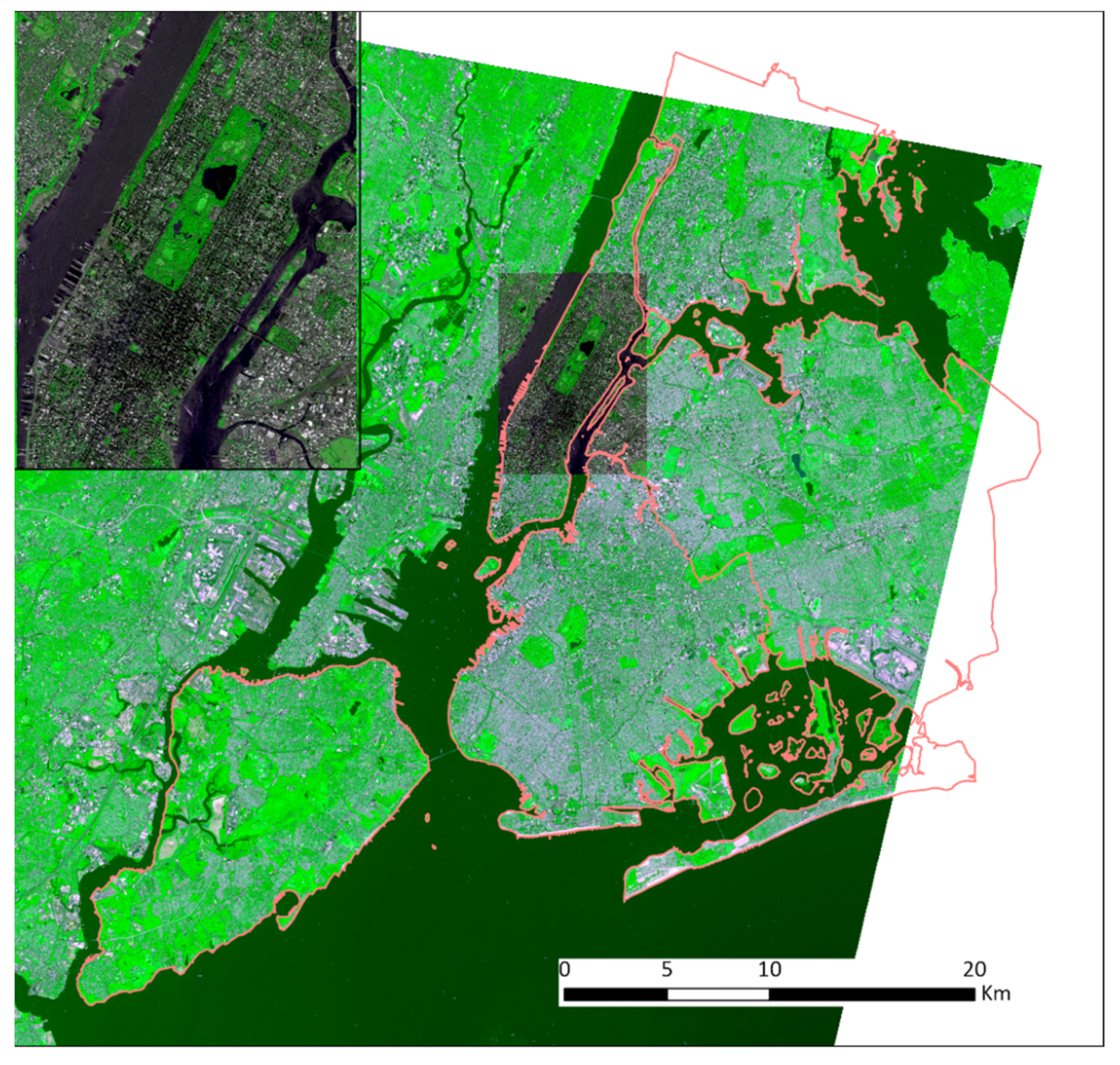
The study area covers New York City (NYC) and its metropolitan region (Figure 1). A true-color composite of ASTER satellite (15 m spatial resolution) shows the fine detail of urban structures: vegetation in green, urban areas in white/gray, and water in black (Figure 1). The residential areas are scattered, shown as bright spots mixed with green trees on the streets. At the center is Manhattan, with a bright green oasis (Central Park) in the middle. Manhattan is the center of the financial district with many tall buildings mainly located south of Central Park in the downtown and midtown region (Figure 1 inset map). The dark color represents the shadows cast by the high-rise buildings. The mixed bright and dark spots in the west part of the midtown are lower-rise buildings. The Hudson River runs north to south and separates New Jersey (on the left) from Manhattan Island (on the right). The Harlem River at the north of Manhattan separates Manhattan from the Bronx. The Harlem River merges with the East River and separates Manhattan from Queens in the east and Brooklyn in the southeast. Following the direction to which Manhattan points is the Staten Island. In the suburban region, green vegetation is scattered in the residential backyards. The industrial areas shown in bright and dark spots are located at the intersection between Queens and Brooklyn, next to the East River.
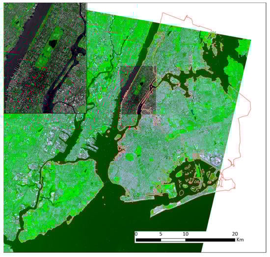
Figure 1.
Overview of the study area showing true-color EOS-Terra ASTER satellite image of the New York City Metropolitan area observed on 8 September 2002. True-color QuickBird satellite image of Manhattan and its surrounding area was observed on 2 August 2002 (inset map).
The climate is controlled by cold, dry air mass movement from the north and warm, humid air mass movement from the south. In addition to the above two air masses’ interactions, the air mass flow from the North Atlantic Ocean produces cool, cloudy, and moist weather conditions in the NYC metropolitan area. The land-sea temperature differences in all seasons have a strong local impact on NYC climate. Land-sea breezes cool NYC on warm spring and summer days and warm NYC on cold nights in autumn, winter, and early spring [24]. Surface elevation increases from the coast to inland. In the NYC metropolitan region, two ridges are parallel to the coastline (Figure 2a). One is along the boundary between Brooklyn and Queens, and the other is on the west side of the Hudson River. Each ridge blocks the cooler land-sea breeze when moving from the coast to inland, resulting in warmer surface temperatures (Figure 2b).
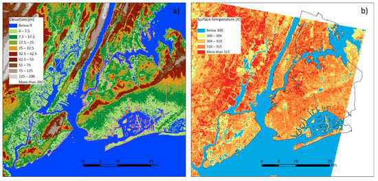
Figure 2.
The maps showing: (a) The topography of New York City (at 30 m spatial resolution), ridges can be seen in the map, and (b) ASTER surface temperature (K) over New York City and surrounding locations on 8 September 2002.
3. Materials and Methods
3.1. Data Source
Advanced Spaceborne Thermal Emission and Reflection Radiometer (ASTER) surface kinetic temperature data (level 2) was downloaded from NASA [25,26]. The temperature and emissivity separation algorithm accurately retrieves surface temperature using the thermal infrared (TIR) bands [27]. The spatial resolution of ASTER surface temperature is 90 m and has an accuracy of 1.5 Kelvin. The QuickBird images (spatial resolution of 2.8 m) were used to produce the detailed land cover classification. During the time of satellite data acquisition, the weather was clear and cloud-free (Table 1). Both the images were collected within a month apart, in August–September 2002, for consistency, while recent ECOSTRESS data [28] was used to observe UHI mitigation effects on land surface temperature in our study area. The date of pass of the ECOSTRESS satellite is 27 August 2020. The time of pass in all images is consistent and collected around 4 pm local time (EST). The ASTER and ECOSTRESS surface temperature product is corrected for emissivity. In contrast, the emissivity used in the Landsat surface temperature product was interpolated from ASTER Global Emissivity Database (GED) data for the spatial grid and spectral bands and thus is not used for this study.

Table 1.
Details of satellite data product used in this study.
The Shuttle Radar Topography Mission (SRTM) elevation at one arc-second (~30 m spatial resolution) was downloaded from NASA Earth Explorer. In addition, parcel (tax lot) level urban structural information and the building footprint data were downloaded from the NYC Department of City Planning [29]. The urban structural parameters include building footprint area, building classes, land use category, commercial area, residential area, total floors, building heights, and year built. According to the year built, more than 95% of the buildings were built before 2000. Tree census data of 2005 in NYC census tracts were also used in the analysis [30].
3.2. Image Classification
Urban areas represent a wide range of land uses and surface properties. To fully understand the spatial characteristics of urban structural and anthropogenic factors and the feedback to human-dominated urban ecosystems, we classified the urban areas into different surface types. The most common subdivisions of urban areas are residential (low, medium, and high), industrial, and commercial areas [31]. Each subdivision has distinct surface morphological characteristics defined by the amounts and types of vegetation and the size or roughness of different elements. These differences result in variations of flux partitioning across a city and the development of distinct micro- to local-scale climates. This study used a slightly different classification scheme for various urban components following Gluch et al. [32]. The classification of different urban components was based on the spectral reflectance of blue, green, red, and near-infrared wavelengths measured by the QuickBird satellite. We did this to capture finer details of urban compositions and address fine-scale surface temperature patterns in the study area.
We used a supervised approach to classify high-resolution QuickBird imagery into various urban land categories (bright, medium, and dark impervious surfaces, shadows, water, trees/shrubs, grassland, and bareground). We used the Fuzzy ARTMAP for classification, a neural network developed by Carpenter [33]. This algorithm has been widely used for satellite image classification [34,35,36]. The ARTMAP is a match-based learning neural network that uses a self-organizing arbitrary system to map inputs to outputs. It also has attractive features such as being fast and stable [34,35].
The classes were chosen based on spectral differentiation (Table 2). The analysis was carried out based on vegetation leaf-on conditions [32]. The descriptions of these classes are as follows: (1) Shadow class: A standalone category. The selection of shadow classes attempts to separate impervious dark and shadow classes since they can constitute different thermal properties. (2) Water class: In this class, all water bodies present within the study are included, regardless of water depth. However, we masked out the water body during the classification. (3) Trees class: This category includes vegetation that can cast a shadow. Such as deciduous and evergreen trees and shrubs with greater canopy cover. (4) Grassland class: This class includes grasses in residential lawns, parks, sides of streets, and golf courses. The reflectance of this class in the near-infrared band is the highest among all classes due to its continuous, photosynthetically active canopy [32]. (5) Bright cover class: The bright cover refers to surfaces with a high albedo, such as highly reflective rooftops and industrial plants. (6) and (7) Impervious-medium and dark classes: The impervious-medium surfaces are mainly concrete materials, while dark surfaces are mainly asphalt, tar, parking lots, and roadways. The dark surfaces appear brighter than shadows. (8) Bareground class: This class typically refers to playing fields and empty lots.
Table 2.
The land-use categories are delineated based on the spectral signature using Fuzzy ARTMAP [33].
As per the class description, we selected training areas for shadows, bright cover, impervious-medium and dark surfaces, trees, grassland, and bareground (Table 2). The spatial resolution of the QuickBird image is fine enough to distinguish these individual features represented by urban materials such as pavement, rooftops, trees, or bareground.
3.3. Accuracy Assessment
To quantitatively evaluate the accuracy of our image classification results, we used both confusion matrix and further visual interpretation. To create the confusion matrix, we recollected our ground truth from the original image through visual interpretation and our knowledge of New York City. The ground truth used to create a confusion matrix is entirely independent of the training sites for our classification algorithm. In reality, the confusion matrix is not a panacea for classification accuracy assessment [37]. We collected large homogeneous areas as ground truth and avoided mixed or heterogeneous regions. The accuracy assessed using the confusion matrix tends to be overestimated. This problem is even worse for the urban area due to the small scale of the urban structure, resulting in many mixed pixels even for high-resolution QuickBird images.
Most of the pixels are correctly classified. Some grasslands are misclassified as impervious-medium surfaces, while some impervious-dark surfaces are misclassified as impervious-medium surfaces or the shadow category (Table 3). A few tree pixels are classified as grassland, a few impervious-medium surface pixels are classified as bright surfaces, and a small part of bright surfaces are misclassified as impervious-medium surfaces. Overall the classification accuracy is 0.959, and the Kappa coefficient is 0.947.
Table 3.
The confusion matrix shows the number of correctly and incorrectly classified pixels of the QuickBird image.
For the visual assessment of the shadow category, shapes turned out to be an effective indicator. The shapes of shaded areas projected on the ground should reflect the original shapes of the structures that obscured sunlight. More importantly, they should incline to the specific direction precisely opposite of the Sun’s position. For instance, the dark rectangular area which does not align with the Sun’s direction was almost automatically eliminated from the shadow category. The shadow cover includes the shadows cast by both trees and buildings. Our visual interpretation indicates that we classify the shadow category very well.
3.4. Data Processing
The data were cleaned, processed, merged, and analyzed in the python environment. We process the following data for analysis: (1) NYC census tract with demographic information, (2) Parcel level attributes containing building footprint, structural, and land use information, (3) Tree census data containing location information for NYC region, which is filtered for alive trees, (4) Land use classification of QuickBird image, and (5) ASTER surface temperature at 90 m spatial resolution.
The urban land cover compositions derived from the QuickBird image and ASTER surface temperature were co-registered using the co-registration tool in the ENVI software (L3Harris Geospatial). We used zonal statistics functions in the python environment to aggregate ASTER surface temperature at the census tract level. The zonal statistics provide minimum, maximum, mean, and majority, including several other statistical parameters [38]. We aggregated total trees, building area, residential area, commercial area, garage area, and retail areas within each census tract to compare the relationships between surface temperatures and different building attributes. We did spatial join (polygon to polygon) to assign ASTER pixel to each QuickBird pixel to compute fractional cover of different QuickBird land cover classes within each ASTER pixel. The spatial join assigned ASTER pixel to QuickBird pixel that entirely sits within it. This operation discards QuickBird pixel that intersects two and more ASTER pixels to avoid mixed temperature signal. The raster statistics count QuickBird pixel/classes in each ASTER pixel to determine the relationship between urban components and surface temperature. The data provides information on the percentage of each QuickBird class within each ASTER surface temperature pixel of 90 m resolution. We also computed the dominant land use category within each ASTER pixel to check relationships with surface temperature. All the figures were prepared in R studio, ArcGIS Pro 2.8.1, and Python 3.
4. Results
4.1. Satellite-Derived Surface Temperature and Urban Compositions
The ASTER data shows that surface temperature increases from the coast to inland, with cool surface temperatures in Staten Island and South Brooklyn to the warmest in New Jersey in the west (Figure 2b). Three significant areas of surface temperature patterns could be identified, with the coolest coastal regions of Brooklyn, then the warmer Manhattan, Queens, and the Bronx, and the warmest New Jersey areas. These surface temperature patterns correspond to two ridges (Figure 2a), which block the land-sea breeze to bring cooler air inland.
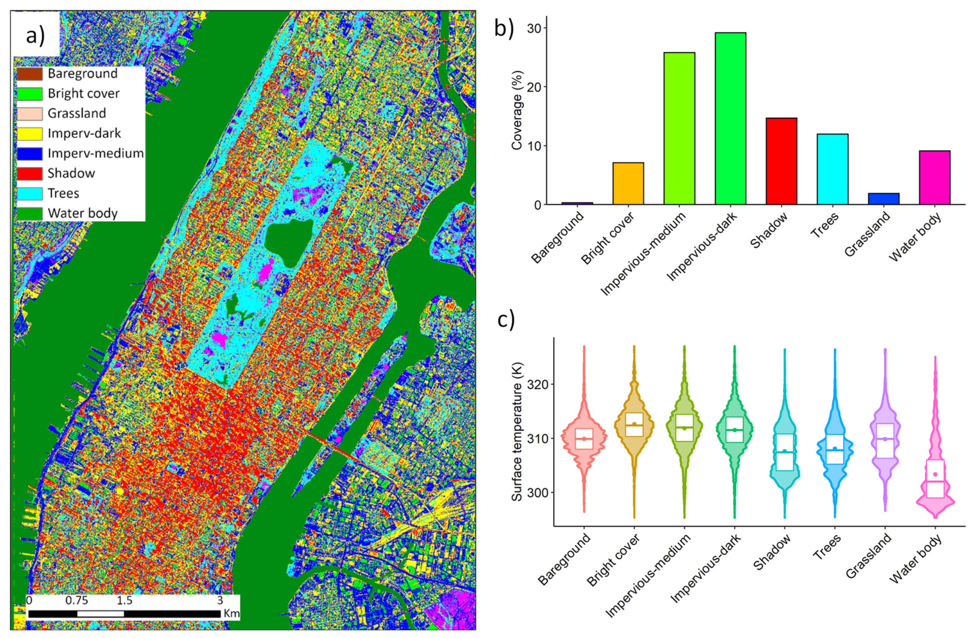
A visual inspection of our supervised classification map of the NYC area (Manhattan and adjoining region) reveals that the distribution of different urban materials and landforms appears to be realistic (Figure 3a). Water bodies are represented by the two rivers and lakes in Central Park, green patches of Central Park, tracts of large paved urban surfaces, and buildings that line the streets are all found at their expected locations. Further, the shadow is well characterized in the downtown Manhattan area, where most high-rise buildings with significant shadow components are located. The lack of bareground class also indicates the efficient use of space in the NYC area, where the land value is relatively high. The impervious-medium and dark surfaces represent the two dominant classes in our study area (Figure 3b). Trees and shadows are the second most dominant classes, followed by water bodies, bright surfaces, and grassland.
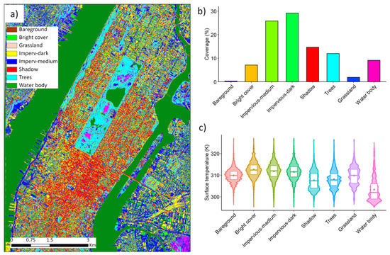
Figure 3.
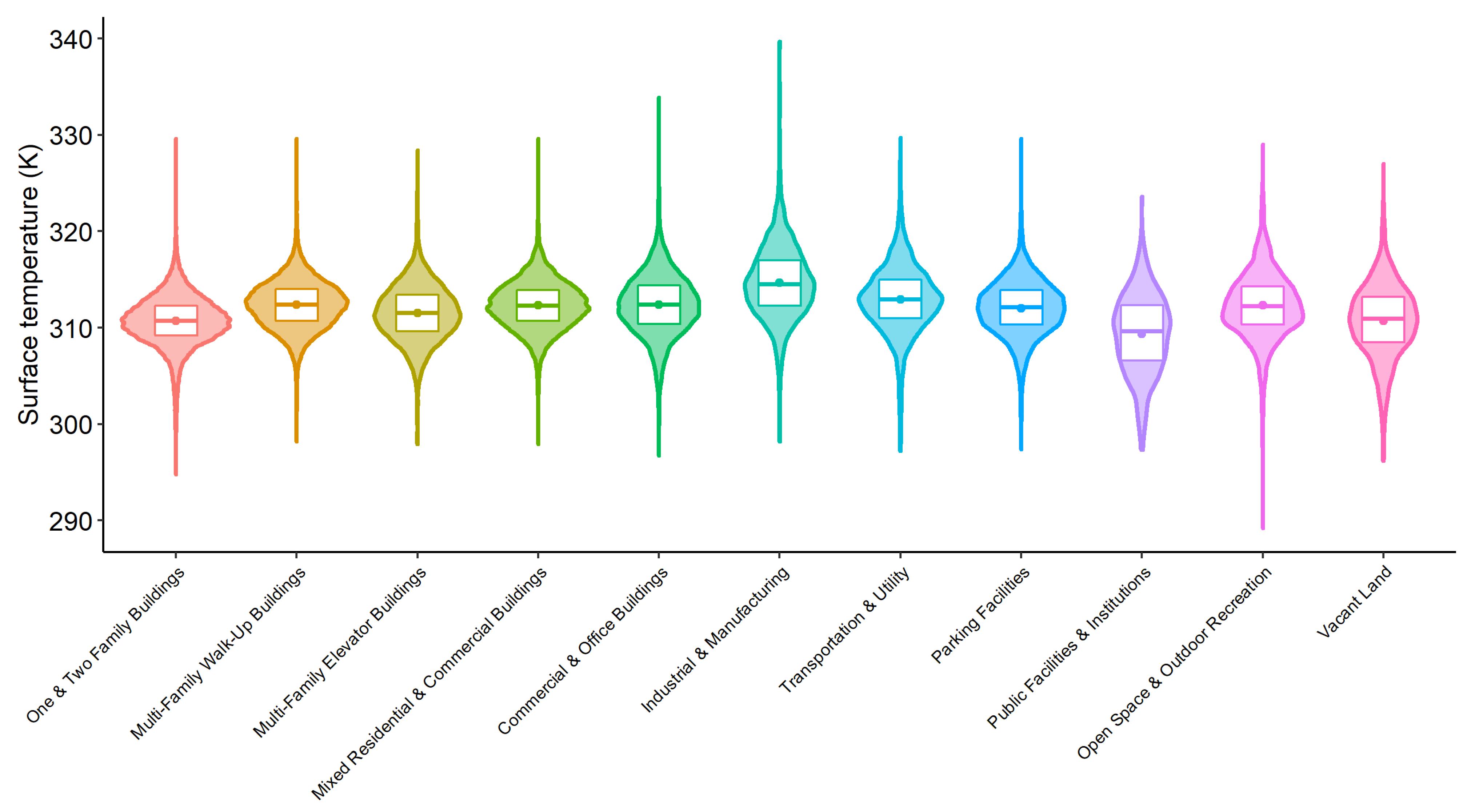
The figure shows: (a) The composition of urban materials obtained by classification of the QuickBird image using Fuzzy ARTMAP neural network scheme, (b) total coverage of urban components in Manhattan and its surrounding area, and (c) Violin chart with boxes represents the interquartile range (IQR) of surface temperature in different urban components. Mean (filled circle) and median (full line inside the box) is also shown.
Bright surfaces have the highest mean surface temperature (312.6 K, median 312.4 K) together with impervious-medium and dark surfaces (mean 311.8 K and 311.5 K, respectively). While the lower mean surface temperature was represented by shadow (307.6 K, median 307.4), typically cast by high-rise buildings, grassland (309.8 K, median 310 K), trees (308.06 K, median 307.8 K), and water bodies (303.3 K, median 302 K). The violin chart with boxes representing interquartile range (IQR) reveals each class’s range and frequencies of surface temperature (Figure 3c). Most of the shadow pixels are in Manhattan, whereas brighter pixels are in Queens. Some of those bright surfaces are industrial plants, which release waste heat. In Manhattan, the dark, heat-trapping materials, like tar roofs and asphalt roads blocked from direct exposure to incoming solar radiation exhibit cooler surface temperatures (Figure 2b and Figure 3a). By contrast, areas to the west of midtown Manhattan and the north of lower Manhattan display much warmer surface temperatures (Figure 2b and Figure 3a). These areas are dominated by low-rise buildings that cast fewer shadows. Three airports in this region, including LaGuardia in Queens, JFK in Brooklyn, and Newark in New Jersey, all show hotspots. These hotspots correspond to the area with large bright impervious surfaces, indicating that large impervious surfaces exhibit greater surface temperature, even if the surface is bright.
4.2. Relationship between Urban Compositions and Surface Temperature
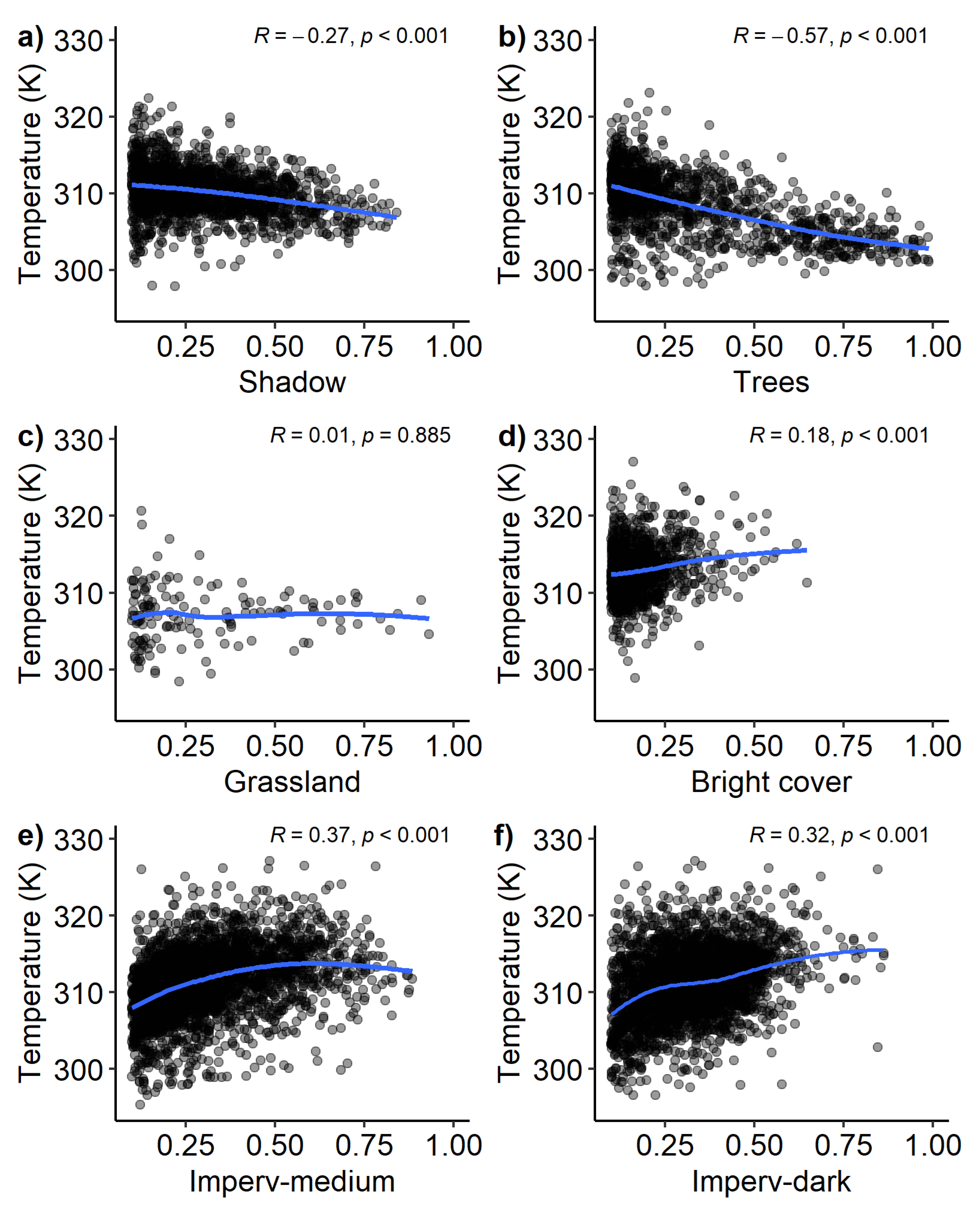
To observe the relationship between fractional urban compositions and surface temperature, we assumed a 10% threshold of each QuickBird class to impact surface temperature in each ASTER pixel substantially. The above threshold was chosen to reduce the noise/mixed-signal effects of the major fraction cover on minor fraction cover. We found greater noise in the bivariate relationships below 10% fraction cover. The analysis revealed that surface temperature decreases with the increase in shadow coverage, with r values of −0.27 and p < 0.01 (Figure 4a). The Sun position when the ASTER data was collected (52-degree Sun elevation) was lower than the Sun position when the QuickBird data was collected (62-degree Sun elevation), so the ASTER image has more shadows than the QuickBird image. As discussed below, this may not affect the relationship between surface temperature and shadows but may add noise to the relationships between surface temperature and impervious surface classes.
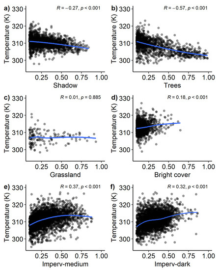
Figure 4.
Relationship between ASTER surface temperature (K) and the fraction of different urban components >10%. Pearson correlation coefficient (R) and level of statistical significance (p values) is shown. Solid lines indicate a locally weighted scatterplot smoothing (LOWESS) function. Sub-plot (a–f) shows individual relationships of urban components with surface temperature.
The surface temperature decreases with tree cover, with a steeper decrease than the shadow class with r values of −0.57 and p < 0.01 (Figure 4b). The relationship between the dominant grassland class and surface temperature is not significant (Figure 4c). Grassland does not significantly reduce and amplify urban heat, consistent with the ground observations conducted in a tropical city by Nichol and Wong [13]. Trees show a greater cooling effect during the day by providing shade than grassland [15,16]. This suggests that the shadow effect and evapotranspiration from trees have a more significant impact on cooling due to their larger leaf area index than grassland; however, it requires further studies at a city-wide scale. Surfaces with bright cover show an increasing surface temperature trend; however, the correlation is not strong but significant, with r values of 0.18 and p < 0.01 (Figure 4d). Usually, bright surfaces with high albedo reflect more and absorb less solar radiation than other impervious surfaces. We expect that surface temperature decrease with bright surface cover. However, due to its low heat capacity, even the bright material can heat the surface easily and quickly. Furthermore, the bright surface is surrounded by heat-trapping surfaces such as impervious-medium and dark surfaces. Those nearby darker impervious materials may amplify and increase the surface temperature with bright covers. Another contributing factor could be that most bright surfaces are rooftops and industrial plants, constantly exposed to the Sun. Therefore, co-existing darker impervious materials within the same ASTER pixel of 90 m spatial resolution contributes to heating effects.
The relationship is quite noisy for the dominant impervious-medium surface class, but the overall surface temperature increases (r values of 0.37 and p < 0.01). However, the slope is not very steep (Figure 4e). The main reason for the noise is that the definition for this class is not very clear, and many impervious-medium surfaces can have different materials. Those materials can have different radiative emission and absorption properties that affect the surface temperature. The surface temperature also increases with the impervious-dark surfaces, with r values of 0.32 and p < 0.01 (Figure 4f). The slope is slightly steeper than the impervious-medium surfaces. Overall, our results show that the r values are not very high, the highest r-value is −0.57 for the shadow category, but the relationships are statistically significant. Low r values are primarily due to the mixed land use category within each ASTER pixel. However, the relationship does show the impact of trees, shadows, and impervious surfaces on surface temperature.
4.3. Impact of Land Use and Building Structure on Surface Temperature
The mean surface temperature for building footprint in the Bronx region is the highest, followed by Brooklyn, Manhattan, and Queens (Figure 5). Building footprint data indicate that the mean surface temperature in Staten Island is the lowest, at least 1.5 K less than that in Queens and 4 K less than that in Bronx and Brooklyn (Figure 5). The violin chart shows the surface temperature distribution in all boroughs; some extreme outliers exist in the data, especially for the Bronx. The median surface temperature in all boroughs is close to their mean concentrations. The analysis further revealed that the industrial and manufacturing land use category has the highest mean and median surface temperature than any other land use category (Figure 6). In addition, transportation and utility, and parking facilities also show higher surface temperature, amongst others. Public facilities and institutions, vacant land, and one and two-family buildings comprise land use categories show the lowest mean and median surface temperature. The choropleth map showed that the heat-generating industrial and manufacturing land use is dominant in southwestern Queens and the Bronx, where surface temperature is more than 313 K (40 °C) and forms a high-temperature hotspot (Figure 7). In Bronx, Brooklyn, and Queens, multi-family walk-up buildings are associated with higher surface temperature clusters. The possibility of anthropogenic factors such as winter heating and summer cooling is likely generating more heat in these localities.
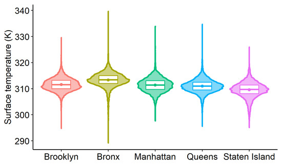
Figure 5.
The violin chart with boxes represents the interquartile range (IQR) of surface temperature in five boroughs of New York City. Mean (filled circle) and median (full line inside the box) is also shown.
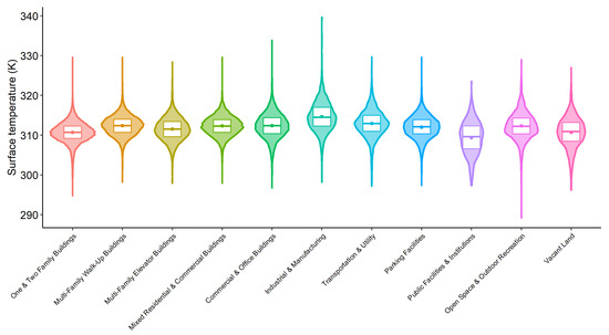
Figure 6.
The violin chart with boxes represents the interquartile range (IQR) of surface temperature in individual building’s land use category in New York City. Mean (filled circle) and median (full line inside the box) is also shown.
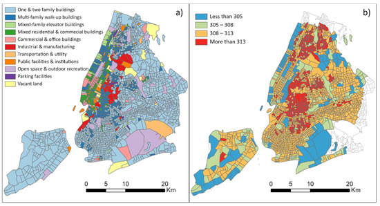
Figure 7.
Choropleth maps show: (a) Dominant building’s land use and (b) surface temperature (mean, K) in different census tracts of New York City.
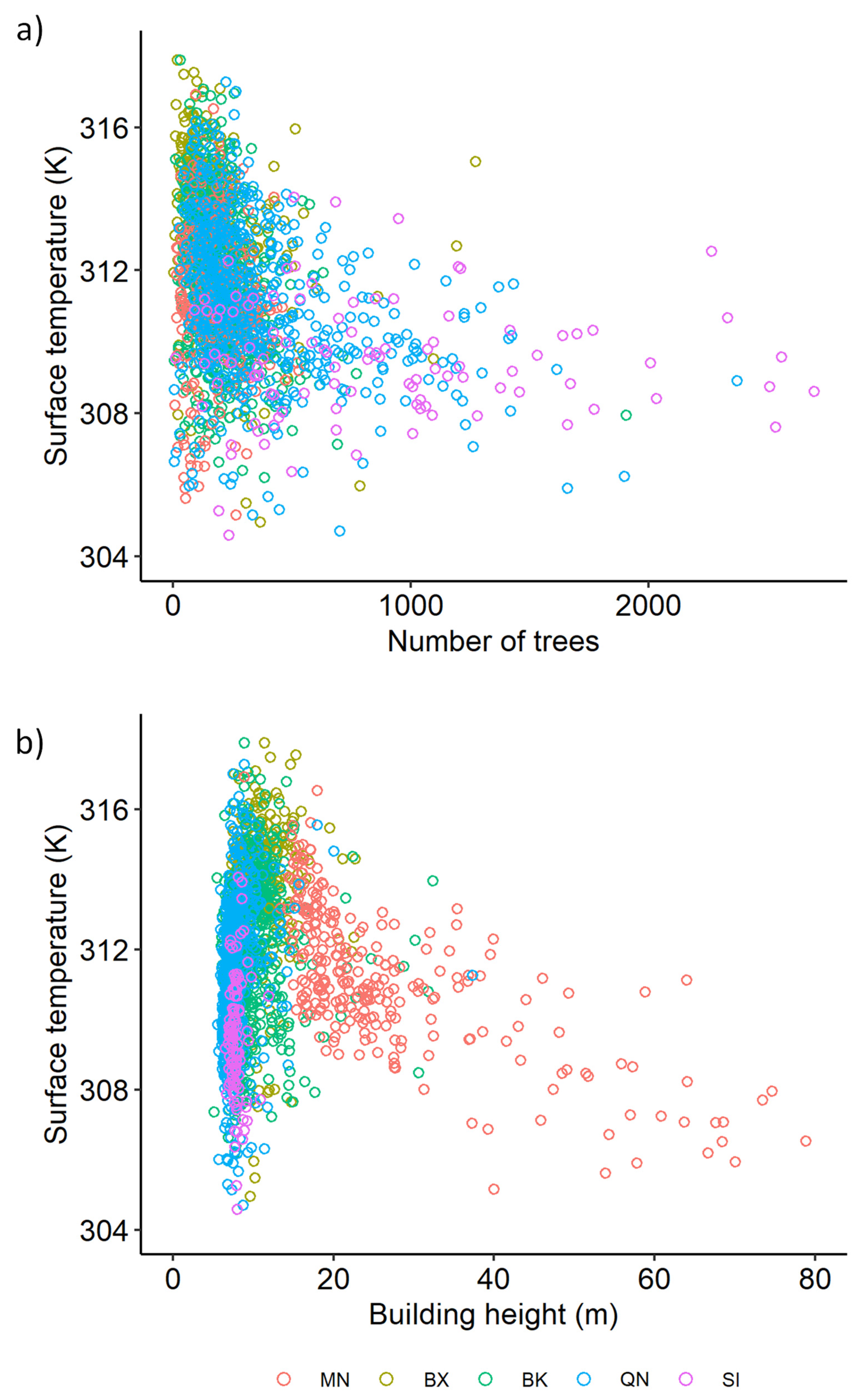
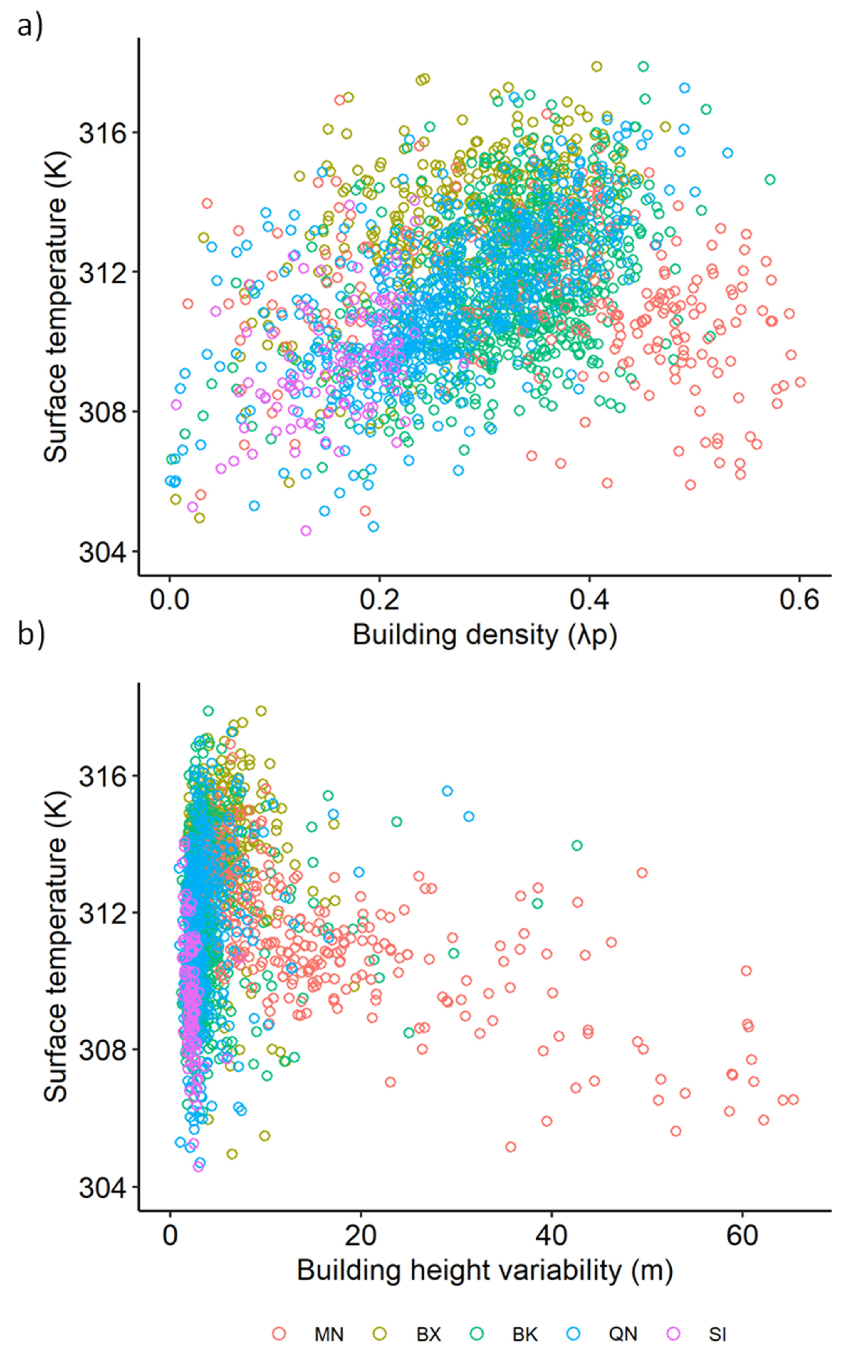
The relationships between surface temperature and the number of trees in different NYC census tracts show that higher surface temperature is associated with lower tree counts, although some exception exists (Figure 8a). Most of the census tracts with lower tree counts are located in Bronx, Brooklyn, and Queens. However, lower tree counts are also associated with lower surface temperatures in some of the census tracts. Those census tracts are primarily located in Manhattan. The scatter plot of the relationship between surface temperature and building height reveals an interesting pattern (Figure 8b). Higher surface temperature is associated with lower building heights (i.e., fewer floors), whereas lower surface temperature is associated with higher building heights (i.e., more floors). We also observed an increase in surface temperatures with building density but showed decreasing trend when density is higher than 0.45 (Figure 9a). The scatter plot also revealed a decrease in surface temperature with higher building height variability (Figure 9b). Most of these census tracts that show a decrease in surface temperature are in Manhattan, where buildings are much taller with more floors and height variability. We also show that census tracts with less building height variability and higher tree counts are associated with lower surface temperature. These results indicate that the larger variations in building heights and trees contribute to lower surface temperature in urban areas of New York City during late summer and early autumn. During this time of the year, the Sun is at a relatively lower elevation. Thereby more shadows are being generated by higher-rise buildings on the surrounding lower-rise buildings and urban heat-trapping surfaces, causing cooling effects. The observed heterogeneity in surface temperature is likely associated with the neighborhood’s specific building land use and structure. We observed that Manhattan has a greater share of high-rise buildings, while Staten Island has more trees than other localities. On the contrary, Bronx, Brooklyn, and Queens have a greater share of industrial and manufacturing land use and multi-family walk-up buildings, including fewer trees.
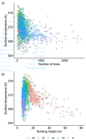
Figure 8.
The scatterplot shows the relationship between: (a) Surface temperature (mean) and the number of trees, and (b) surface temperature (mean) and building height (m) in different census tracts of New York City. Different colors signify boroughs of New York City: MN for Manhattan, BX for Bronx, BK for Brooklyn, QN for Queens, and SI for Staten Island.
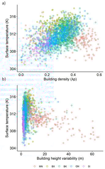
Figure 9.
The figure shows the relationships between: (a) Surface temperature (mean) and building density (ratio of the total building footprint to the land area), and (b) surface temperature (mean) and building height variability (m) in different census tracts of New York City. Different colors signify boroughs of New York City: BK—Brooklyn, BX—Bronx, MN—Manhattan, QN—Queens, and SI—Staten Island.
5. Discussion
Three factors, trees, building heights, and impervious surfaces, including bright surfaces, are primarily responsible for surface temperature heterogeneity in our study site. The replacement of vegetation by heat-trapping and non-porous urban materials alters surface conditions such as albedo, thermal capacity, and heat conductivity. Such transformation alters radiative fluxes between the surfaces and the lower atmosphere [4].
Trees reduce heat in two ways. Firstly, the shadows resulting from the tree control the total amount of radiation absorbed per unit surface area of heat-trapping materials. Secondly, trees return more surface heat to the atmosphere through evapotranspiration and reduce surface temperatures. Similarly, shadows cast by high-rise buildings reduce the amount of solar energy absorbed by the urban heat-trapping surfaces, and so there will be less heating effect. Guo et al. [14] observed a positive impact of building height and density on land surface temperature. They further observed higher land surface temperature associated with medium building height and a lower building density. Krüger et al. [39] showed a direct link between urban climate and building heights. Similarly, we found a slightly higher surface temperature in medium-height buildings (ranging between 10 and 15 m), but the temperature decreases when the heights increase beyond 15 m together with its variability. This indicates that the relationships between surface temperature and urban structure are more likely associated with urban types. Generally, the shadows cast by tall buildings cover large urban impervious surfaces in the areas having more height variability. In addition, because the Sun is at a lower elevation in September cause longer shadows in comparison with the summer seasons. Likewise, Zheng et al. [40] observed adverse effects of building heights on land surface temperature in residential areas of Beijing. However, the shadow effect on surface temperature varies with the time of the day and the day of the year.
The shadows from high-rise buildings influence temperature, similar to how vegetation affects surface temperature [41]. Mutual shadows created by tall vegetation, such as in forests, eliminate any existing gaps in forests. Even if some gaps exist between high-rise buildings in cities like New York, the mutual shadows cast on the wall of the buildings and the ground reduces heating effects. Additionally, when the height variability increases, the shadows can effectively cover the adjacent building walls up to hundreds of meters away depending on the Sun’s azimuth [42]. Under such conditions, less incident radiation will likely be absorbed on the urban surfaces (horizontal and/or vertical), leading to cooler urban surfaces. Wang and Xu [12] also indicate that land surface temperature decreases significantly with building height differences and brings a cooling effect.
Our results show that surface temperature increases with increasing fractions of impervious cover (both impervious-medium and dark surfaces). This indicates that dark urban surfaces, mainly low-rise multi-family walk-up buildings with an average number of floors of 3.15, produce fewer shadows contribute to the urban heat. Surfaces with brighter covers show an increasing surface temperature trend. Usually, bright surfaces increase surface albedo, i.e., reflect more and absorb less solar radiation than other impervious surface materials [43]. It is expected that surface temperature would decrease with bright surface cover due to its high albedo. However, due to its low heat capacity, even the bright impervious surface can heat the surface easily and quickly. Most bright surfaces are rooftops and industrial plants, which are constantly exposed to the Sun. Moreover, the bright surface is surrounded by dark and medium-dark heat-trapping surfaces. The presence of these heat-trapping darker materials may amplify the surface temperature. For the impervious-dark and impervious-medium surfaces and roofs, not much light penetrates the surfaces, incident radiation is not reflected back to the atmosphere is used to heat the surfaces, causing increased surface temperature. Using high spatial resolution satellite data, we characterized the shadows, green vegetation, impervious surfaces, and their brightness and identified each component’s impact on surface temperature in our study site.
Using building footprint data at the parcel level combined with high-resolution satellite images, we identified the effects of different urban components such as shadows, green vegetation, building heights, building density, impervious surfaces, and their brightness on surface temperature. Building footprint data reinforces the satellite-derived interpretation of finer-scale surface temperature variations in urbanized settings and determines the likely causes. Our analysis indicates that shadows cast by high-rise buildings containing multiple floors and trees reduce UHI effects. In contrast, impervious-medium and impervious-dark surfaces, typically low-rise multi-family walk-up buildings, and brighter industrial and manufacturing areas increase UHI.
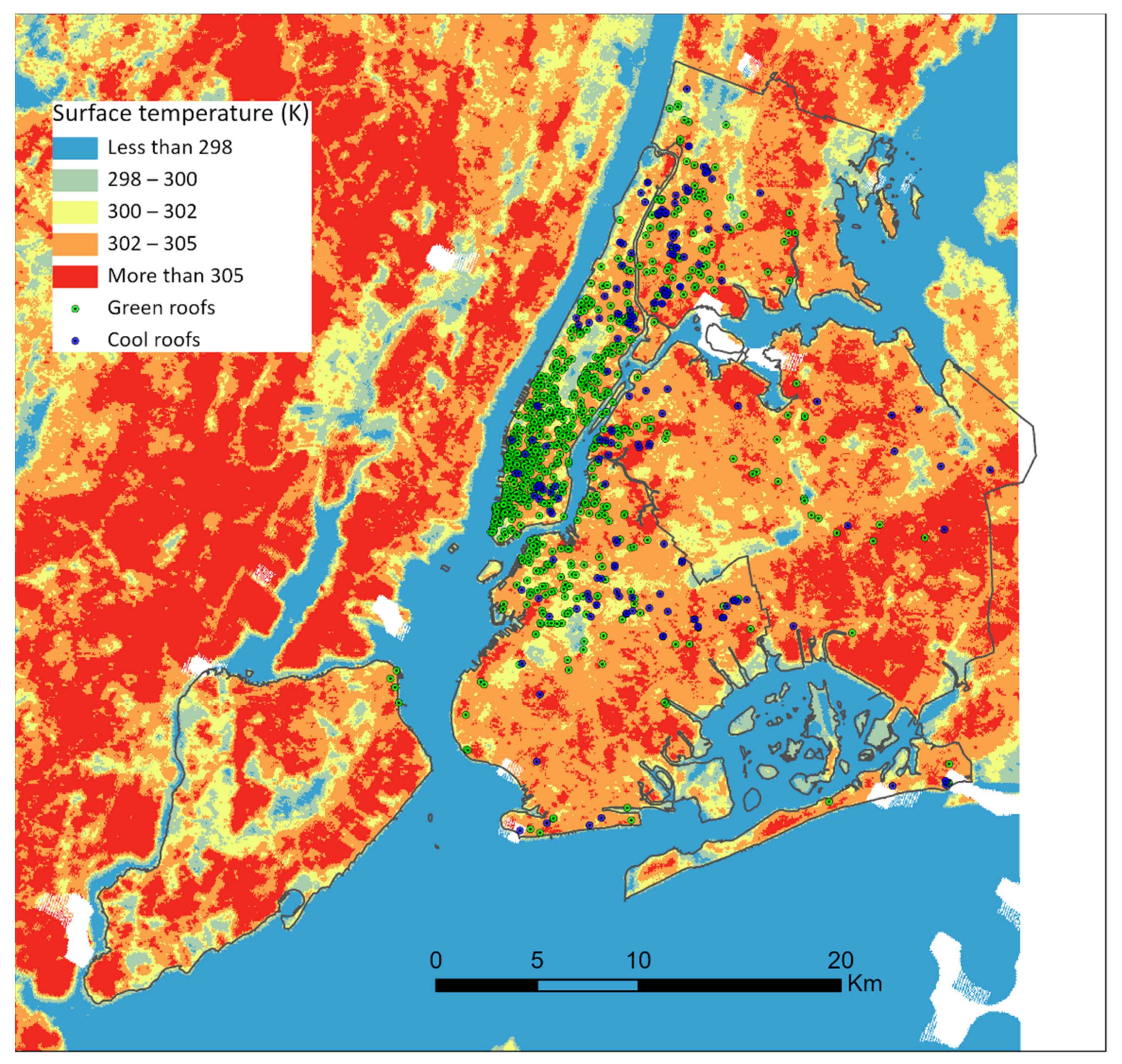
Various environmental and governmental agencies are working towards mitigating the UHI effect. Two approaches are being adopted. One uses highly reflective materials for roofs and pavements, and the other planting trees. The green roof programs are being conducted and tested in several big cities, including New York City [44]. Green roofs impact stormwater use and help release heat absorbed on roof surfaces and cool overall surface temperature. In addition, New York City adopted cool roof projects by whitening the black asphalt rooftops and make them highly reflective to reduce surface temperature [45]. Our study indicates that trees and grasses can mitigate UHI. However, most green roof projects are implemented in Manhattan, where ASTER data showed much cooler surface temperatures in late summer/early autumn of 2002. The analysis of building footprint data further revealed that NYC urban structure had not changed significantly (95% of the buildings aged more than 20 years) except for the green roof and cool roof project in the past 20 years. Recent land surface temperature data retrieved by ECOSTRESS revealed UHI hotspots in the same areas observed in 2002, especially the Bronx, southeastern Queens, Brooklyn, and the industrial regions of Queens (Figure 10). The NYC never gets direct overhead sunlight throughout the year and composes many tall and skinny buildings. The change of small roof area is likely to have an insignificant impact on temperature observed by satellites. Nevertheless, it is also essential to have a detailed analysis of the seasonal variations in surface temperature patterns and to quantify the long-term impact of green roofs and cool roofs on UHI mitigation in the presence of various influencing factors, such as the areas dominated by multi-family walk-up buildings and industrial and manufacturing land use.
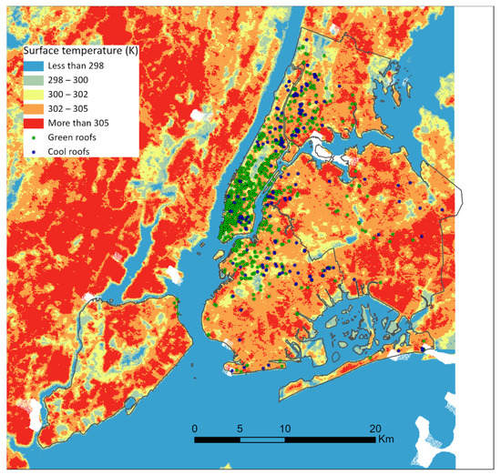
Figure 10.
Maps showing surface temperature (K) measured by ECOSTRESS [28] at 70 m spatial resolution on 27 August 2020. The building locations with cool roofs in 2012 and green roofs in 2016 in New York City.
The future work will involve simulating time-series surface temperature patterns as a function of urban structures, vegetation cover, and shadows derived from high-resolution satellite data for the entire NYC region. It is well known that building shadows show strong seasonality and affect urban land surface temperature [17]. Therefore, we planned to use high-resolution ECOSTRESS images to study the spatiotemporal pattern of urban heat. In particular, we will model the shadow effects due to building height variation and trees on surface temperature patterns. We will combine the locations of cool roofs and green roofs and quantify the cumulative effect on reducing the surface temperature in the city to help design priority locations. Our long-term goal is to assimilate satellite-observed spatiotemporal patterns of urban heat into urban climate models. The shadow analysis would provide helpful information in sustainable urban design, including access to sunlight during different seasons, and help mitigate the impact of climate change. The quantification of UHI effects has a potential public health implication and helps safeguard people from heat-related stress, especially in big cities with high building densities.
6. Conclusions
Our study shows that the trees and shadows cast by high-rise buildings and their variability have a cooling effect. In contrast, more impervious surfaces show a heating effect even in the presence of highly reflective bright surfaces. The census tract with industrial and manufacturing areas and multi-family walk-up buildings as dominant land use categories correspond to the highest mean surface temperature. Buildings with lower heights (fewer floors) and less height variability are associated with higher surface temperature. Although the building density is the highest in Manhattan (the central business district), many tall buildings with variable heights have shown cooling effects. Staten Island has the lowest mean surface temperature amongst all boroughs of New York City, where the number of trees is more. The Bronx has the highest mean surface temperature and constitutes moderate building density, height, and height variability. The finding from this study has an important implication for urban heat island modeling since recent surface temperature image reveals similar hotspot locations as observed 20 years ago. The results show the positive effects of trees and building shadows in reducing urban heat. It could help prioritize the areas to mitigate the UHI effect and reduce associated environmental and health-related costs, including sustainable urban planning.
Author Contributions
Conceptualization, B.N. and W.N.-M.; methodology, B.N., W.N.-M. and M.Ö.; software, B.N. and M.Ö.; formal analysis and data curation, B.N.; writing—original draft preparation, B.N.; writing—review & editing, B.N., W.N.-M. and M.Ö.; funding acquisition, W.N.-M. All authors have read and agreed to the published version of the manuscript.
Funding
This study is funded by NASA grant number 80NSSC20K1718.
Institutional Review Board Statement
Not applicable.
Informed Consent Statement
Not applicable.
Data Availability Statement
ASTER Level 2 Surface Temperature image was downloaded from https://lpdaac.usgs.gov/products/ast_08v003/ (accessed on 28 March 2021). The SRTM elevation at one arc-second (~30 m spatial resolution) was downloaded from NASA Earth Explorer (accessed on 12 March 2021). Building footprint and extensive land use and geographic data at the tax lot level were downloaded from https://www1.nyc.gov/site/planning/data-maps/open-data/dwn-pluto-mappluto.page (accessed on 3 April 2021). Street tree census data were downloaded from https://data.cityofnewyork.us/Environment/2005-Street-Tree-Census/29bw-z7pj (accessed on 5 April 2021). New York City Cool Roofs location was downloaded from https://maps.princeton.edu/catalog/sde-columbia-cul_nyc_dob_coolroofs_2012 (accessed on 9 August 2021). Green roof locations were downloaded from http://doi.org/10.5281/zenodo.1469674 (accessed on 9 August 2021).
Acknowledgments
The authors would like to thank anonymous reviewers for their time and effort in reviewing this paper and improve its quality. We also thank Atsushi Tomita for his help in LULC classification and accuracy assessment. B.N. would like to thank Hunter College of the City University of New York for providing technological support and Ahearn for Python training.
Conflicts of Interest
The authors declare no conflict of interest.
References
- Zhou, B.; Rybski, D.; Kropp, J.P. The role of city size and urban form in the surface urban heat island. Sci. Rep. 2017, 7, 4791. [Google Scholar] [CrossRef] [PubMed]
- Seto, K.C.; Fragkais, M.; Guneralp, B.; Reilly, M.K. A meta-analysis of global urban land expansion. PLoS ONE 2013, 6, e237777. [Google Scholar] [CrossRef] [PubMed]
- Callaghan, A.; McCombe, G.; Harrold, A.; McMeel, C.; Mills, G.; Moore-Cherry, N.; Cullen, W. The impact of green spaces on mental health in urban settings: A scoping review. J. Ment. Health 2021, 30, 179–193. [Google Scholar] [CrossRef]
- Oke, T.R. The energetic basis of the urban heat island. Q. J. R. Meteor. Soc. 1982, 108, 1–24. [Google Scholar] [CrossRef]
- Tan, H.; Ray, P.; Tewari, M.; Brownlee, J.; Ravindran, A. Response of Near-Surface Meteorological Conditions to Advection under Impact of the Green Roof. Atmosphere 2019, 10, 759. [Google Scholar] [CrossRef] [Green Version]
- Zhou, D.; Xiao, J.; Bonafoni, S.; Berger, C.; Deilami, K.; Zhou, Y.; Frolking, S.; Yao, R.; Qiao, Z.; Sobrino, J.A. Satellite Remote Sensing of Surface Urban Heat Islands: Progress, Challenges, and Perspectives. Remote Sens. 2019, 11, 48. [Google Scholar] [CrossRef] [Green Version]
- Voogt, J.A.; Oke, T.R. Thermal remote sensing of urban climates. Remote Sens. Environ. 2003, 86, 370–384. [Google Scholar] [CrossRef]
- Voogt, J.A.; Oke, T.R. Complete urban surface temperatures. J. Appl. Meteorol. 1997, 36, 1117–1132. [Google Scholar] [CrossRef]
- Deilami, K.; Kamruzzaman, M.; Liu, Y. Urban heat island effect: A systematic review of spatio-temporal factors, data, methods, and mitigation measures. Int. J. Appl. Earth Obs. Geoinf. 2018, 67, 30–42. [Google Scholar] [CrossRef]
- Yoshikado, H. Vertical structure of the sea breeze penetrating through a large urban complex. J. Appl. Meteor. 1990, 29, 878–891. [Google Scholar] [CrossRef] [Green Version]
- Yoshikado, H. Numerical study of the daytime urban effect and its interaction with the sea breeze. J. Appl. Meteor. 1992, 31, 1146–1164. [Google Scholar]
- Wang, M.; Xu, H. The impact of building height on urban thermal environment in summer: A case study of Chinese megacities. PLoS ONE 2021, 16, e0247786. [Google Scholar] [CrossRef]
- Nichol, J.; Wong, M.S. Modeling urban environmental quality in a tropical city. Landsc. Urban Plan. 2005, 73, 49–58. [Google Scholar] [CrossRef]
- Guo, G.; Zhou, X.; Wu, Z.; Xiao, R.; Chen, Y. Characterizing the impact of urban morphology heterogeneity on land surface temperature in Guangzhou, China. Environ. Model. Softw. 2016, 84, 427–439. [Google Scholar] [CrossRef]
- Armson, D.; Stringer, P.; Ennos, A.R. The effect of tree shade and grass on surface and globe temperatures in an urban area. Urban. For. Urban. Green. 2012, 11, 245–255. [Google Scholar] [CrossRef]
- Edmondson, J.; Stott, I.; Davies, Z.; Gaston, K.J.; Leake, J.R. Soil surface temperatures reveal moderation of the urban heat island effect by trees and shrubs. Sci. Rep. 2016, 6, 33708. [Google Scholar] [CrossRef] [Green Version]
- Yu, K.; Chen, Y.; Wang, D.; Chen, Z.; Gong, A.; Li, J. Study of the Seasonal Effect of Building Shadows on Urban Land Surface Temperatures Based on Remote Sensing Data. Remote Sens. 2019, 11, 497. [Google Scholar] [CrossRef] [Green Version]
- Loughner, C.P.; Allen, D.J.; Zhang, D.L.; Pickering, K.E.; Dickerson, R.R.; Landry, L. Role of urban tree canopy and buildings in urban heat island effects: Parameterization and preliminary results. J. Appl. Meteor. 2012, 51, 1775–1793. [Google Scholar] [CrossRef]
- Lin, T.P.; Matzarakis, A.; Hwang, R.L. Shading effect on long-term outdoor thermal comfort. Build. Environ. 2010, 45, 213–221. [Google Scholar] [CrossRef]
- Roth, M.; Oke, T.R.; Emery, W.J. Satellite-derived urban heat islands from three coastal cities and the utilization of such data in urban climatology. Int. J. Remote Sens. 1989, 10, 1699–1720. [Google Scholar] [CrossRef]
- Carlson, T.N. Regional-scale estimates of surface moisture availability and thermal inertia using remote thermal measurements. Remote Sens. Rev. 1986, 1, 197–247. [Google Scholar] [CrossRef]
- Price, J.C. Assessment of the urban heat island effect through the use of satellite data. Mon. Wea. Rev. 1979, 107, 1554–1557. [Google Scholar] [CrossRef] [Green Version]
- Voogt, J.A.; Grimmond, C.S.B. Modeling surface sensible heat flux using surface radiative temperatures in a simple urban area. J. Appl. Meteorol. 2000, 39, 1679–1699. [Google Scholar] [CrossRef]
- Gedzelman, S.D.; Austin, S.; Cermak, R.; Stefano, N.; Partridge, S.; Quesenberry, S.; Robinson, D.A. Mesoscale aspects of the Urban Heat Island around New York City. Theor. Appl. Climatol. 2003, 75, 29–42. [Google Scholar] [CrossRef]
- ASTER_08, 2020. NASA/METI/AIST/Japan Spacesystems and U.S./Japan ASTER Science Team. In ASTER Level 2 Surface Temperature Product; Distributed by NASA EOSDIS Land Processes DAAC; DAAC: Sioux Falls, SD, USA, 2001. [CrossRef]
- Yamaguchi, Y.; Kahle, A.; Tsu, H.; Kawakami, T.; Pniel, M. Overview of Advanced Spaceborne Thermal Emission and Reflection Radiometer (ASTER). IEEE Trans. Geosci. Remote Sens. 1998, 36, 1062–1071. [Google Scholar] [CrossRef] [Green Version]
- Gillespie, A.R.; Matsunaga, T.; Rokugawa, S.; Hook, S.J. Temperature and Emissivity Separation from Advanced Spaceborne Thermal Emission and Reflection Radiometer (ASTER) Images. IEEE Trans. Geosci. Remote Sens. 1998, 36, 1113–1126. [Google Scholar] [CrossRef]
- Hook, S.; Hulley, G. ECOSTRESS Land Surface Temperature and Emissivity Daily L2 Global 70 m V001; NASA EOSDIS Land Processes DAAC: Sioux Falls, SD, USA, 2018. [Google Scholar] [CrossRef]
- New York City Department of City Planning (NYC DCP). PLUTO: Extensive Land Use and Geographic Data at the Tax Lot Level. 2020. Available online: https://www1.nyc.gov/site/planning/data-maps/open-data/dwn-pluto-mappluto.page (accessed on 9 March 2021).
- New York City Department of Environmental Protection (NYC DEP). 2005 Street Tree Census, NYC Open Data. Available online: https://data.cityofnewyork.us/Environment/2005-Street-Tree-Census/29bw-z7pj (accessed on 9 March 2021).
- Loveland, T.; Belward, A. The IGBP-DIS global 1 km land cover data set, DISCover: First results. Int. J. Remote Sens. 1997, 18, 3289–3295. [Google Scholar] [CrossRef]
- Gluch, R.; Quattrochi, D.A.; Luvall, J.C. A multi-scale approach to urban thermal analysis. Remote Sens. Environ. 2006, 104, 123–132. [Google Scholar] [CrossRef]
- Carpenter, G.A.; Grossberg, S.; Markuzon, N.; Reynolds, J.H.; Rosen, D.B. Fuzzy ARTMAP: A neural network architecture for incremental supervised learning of analog multidimensional maps. IEEE Trans. Neural Netw. 1992, 3, 698–713. [Google Scholar] [CrossRef] [Green Version]
- Carpenter, G.; Gopal, A.S.; Macomber, S.; Martens, S.; Woodcock, C.E. A neural network method for mixture estimation for vegetation mapping. Remote Sens. Environ. 1999, 70, 138–152. [Google Scholar] [CrossRef] [Green Version]
- Carpenter, G.A.; Gopal, S.; Macomber, S.; Martens, S.; Woodcock, C.E. A neural network method for efficient vegetation mapping. Remote Sens. Environ. 1999, 70, 326–338. [Google Scholar] [CrossRef] [Green Version]
- Pax-Lenney, M.; Woodcock, C.E.; Macomber, S.A.; Gopal, S.; Song, C. Forest mapping with a generalized classifier and Landsat TM data. Remote Sens. Environ. 2001, 77, 241–250. [Google Scholar] [CrossRef]
- Friedl, M.A.; Woodcock, C.E.; Gopal, S.; Muchoney, D.; Strahler, A.H.; Barker-Schaaf, C. A Note on procedures used for accuracy assessment in land cover maps derived from AVHRR data. Int. J. Remote Sens. 2000, 21, 1073–1077. [Google Scholar] [CrossRef]
- Rasterstat. Zonal Statistics: A Method of Summarizing and Aggregating the Raster Values Intersecting a Vector Geometry. 2021. Available online: https://pythonhosted.org/rasterstats/index.html (accessed on 28 March 2021).
- Krüger, E.L.; Minella, F.O.; Rasia, F. Impact of urban geometry on outdoor thermal comfort and air quality from field measurements in Curitiba, Brazil. Build. Environ. 2011, 46, 621–634. [Google Scholar] [CrossRef]
- Zheng, Z.; Zhou, W.; Yan, J.; Qian, Y.; Wang, J.; Li, W. The higher, the cooler? Effects of building height on land surface temperatures in residential areas of Beijing. Phys. Chem. Earth 2019, 110, 149–156. [Google Scholar] [CrossRef]
- Ni, W.; Li, X.; Woodcock, C.E.; Caetano, M.R.; Strahler, A.H. An Analytical Hybrid GORT Bidirectional Reflectance Model for Discontinuous Plant Canopies. IEEE Trans. Geosci. Remote Sens. 1999, 37, 987–999. [Google Scholar]
- Vo, A.V.; Laefer, D.F. A bid data approach for comprehensive urban shadow analysis from airborne laser scanning point clouds. In Proceedings of the ISPRS Annals of the Photogrammetry, Remote Sensing and Spatial Information Sciences, 14th 3D GeoInfo Conference, Singapore, 24–27 September 2019; Volume IV-4/W8. [Google Scholar]
- Deng, Y.; Chen, R.; Xie, Y.; Xu, J.; Yang, J.; Liao, W. Exploring the Impacts and Temporal Variations of Different Building Roof Types on Surface Urban Heat Island. Remote Sens. 2021, 13, 2840. [Google Scholar] [CrossRef]
- Treglia, M.L.; McPhearson, T.; Sanderson, E.W.; Yetman, G.; Maxwell, E.N. Green Roofs Footprints for New York City, Assembled from Available Data and Remote Sensing (Version 1.0.0). Zenodo. 2018. Available online: https://github.com/tnc-ny-science/NYC_GreenRoofMapping/blob/master/greenroof_gisdata/CurrentDatasets/GreenRoofData2016_20180917.csv (accessed on 9 August 2021).
- New York City Cool Roofs (NYC CoolRoofs). Research Data Services (RDS), Columbia University Libraries and New York City Department of Buildings. Available online: https://maps.princeton.edu/catalog/sde-columbia-cul_nyc_dob_coolroofs_2012 (accessed on 9 August 2021).


Publisher’s Note: MDPI stays neutral with regard to jurisdictional claims in published maps and institutional affiliations. |
© 2021 by the authors. Licensee MDPI, Basel, Switzerland. This article is an open access article distributed under the terms and conditions of the Creative Commons Attribution (CC BY) license (https://creativecommons.org/licenses/by/4.0/).