Investigation on Global Distribution of the Atmospheric Trapping Layer by Using Radio Occultation Dataset

Abstract

The trapping layer refers to the atmospheric layer with vertical gradient of atmospheric refractivity less than −157 N-Units/km or vertical gradient of atmospheric modified refractivity 0 M-unit/km, which has a significant impact on radar and radio communication systems. Based on COSMIC and other radio occultation data, we show the statistical characteristics of the global trapping layer during 2005–2020.The statistical results show that the occurrence rate of the trapping layers is mainly concentrated between 50°S and 50°N, and higher occurrences of the trapping layers with more than 50% mainly occur in the boundary area between ocean and land, such as the northwest coastal area of Mexico, the west coastal area of Africa, the Mediterranean Sea, the Red Sea and the Arabian Sea, and the northwest area of Australia, etc. The altitude of the trapping layer is lower near the land and increases with the distance away from the coastline. The intensity is mainly between 6 M-unit and 24 M-unit (an M-unit is the unit of atmospheric modified refractivity), and the average value in some regions is above 24 M-unit, such as in the Arabian Sea area. In addition, the thickness of the trapping layer is between 50 and 240 m, and is generally larger over the ocean than over the land. These results reveal that the generation of the trapping layer is the result of the interaction of various background environmental factors such as radiation band migration, trade winds, monsoons, solar radiation heating, sea–land breezes and so on.

1. Introduction

Atmospheric super-refraction phenomena associated with sharp gradients in temperature and water vapor pressure frequently occur in the near-Earth atmospheric boundary layer, especially near coastal and ocean areas [1,2]. Ao et al. [3] indicated that there is an atmospheric trapping layer when the vertical gradient of atmospheric refractivity is $\mathrm{dN}/\mathrm{dh}<-157$ N-Units/km or vertical gradient of atmospheric modified refractivity is$\mathrm{dM}/\mathrm{dh}<0$ M-unit/km, which significantly affects the performance of radio communication systems by changing the propagation path and attenuation characteristics of electromagnetic waves. The trapping layer is always embedded inside the duct, which produces information on the sharp layer and is related to the physical processes or conditions that form the duct [3,4]. The generation and distribution of the atmospheric trapping layer are closely related to the geography and meteorological water level conditions such as nocturnal radiation cooling, warm and dry land air passing over a cooler sea, sea–land breezes, monsoon and so on [5,6]. Studying the characteristics of the trapping layer and its influence on the propagation of electromagnetic waves is helpful to accurately assess the influence of the complex duct environment on the radio information system, and provide environmental analysis information and auxiliary decision-making methods for system design and development.

Statistical studies of the occurrence of the atmospheric trapping layer in different regions have been carried out in the last few decades [7,8,9,10]. By using 6-year European Centre for Medium-Range Weather Forecasts (ECMWF) data, Engeln [8] calculated the atmospheric refractivity and analyzed the seasonal variations in the occurrence rate, altitude, thickness, and gradient of the trapping layer at a height of 0~2.5 km. The observed results shown in Engeln [8] show that the distribution of the trapping layer occurrence has obvious seasonal variations, which are mainly affected by stratocumulus, fog, monsoon and boundary layer inversions in temperature and moisture [11,12,13,14]. However, ECMWF data have some limitations. The resolution of ECMWF data decreases with altitude, making trapping layer information from above 2.5 km is almost useless. The vertical resolution of ECMWF data is greater than 200 m where the height is over 1 km, and it can only detect some thicker trapping layers.

Atmospheric parameter profiles, such as atmospheric refractivity, temperature, pressure and humidity, can be measured by using radio occultation technology [15]. When the MicroLab-1 satellite was launched in 1995, Global Positioning System (GPS) radio occultation measurements were first applied to the study of global atmospheric distribution characteristics [16]. Subsequently, CHAMP [17] and SAC-C [18] equipped with GPS radio occultation receivers were successfully launched. Following the launch of COSMIC on 14 April 2006, approximately 2000 to 3000 atmospheric radio occultation profiles can now be obtained every day [19,20]. The large amount of COSMIC radio occultation data available is beneficial for studying the global distributions of the trapping layer occurrence rate. The vertical resolution of the COSMIC data is 100 m, which allows researchers to observe some of the finer structures of the trapping layer, which is helpful for investigating the generation mechanism of the trapping layer. It is noted that the number of RO profiles has declined greatly recently. Due to its significant advantages of high precision, high vertical resolution, and ability to perform all-weather observations [21,22,23], we firstly investigate the temporal and spatial distribution characteristics of the global trapping layer based on the GPS radio occultation dataset. COSMIC and other radio occultation data are used in this study. The data source and research methods are introduced in Section 2. In Section 3, we analyze the results of the temporal and spatial distribution of the trapping layer characteristics. Our conclusions are summarized in Section 4.

2. Method and Data

2.1. Method Description

Radio waves are affected by atmospheric refraction during propagation, and refraction effects must be considered in the actual propagation process. The refractivity is determined by pressure, temperature and humidity [24]:

$$\mathrm{N}=\frac{77.6}{\mathrm{T}}\left(\mathrm{p}+\frac{4810\mathrm{e}}{\mathrm{T}}\right)$$

(1)

where, $\mathrm{p}$ is atmospheric pressure (hPa), $\mathrm{T}$ is temperature (K), and $\mathrm{e}$ is water vapor pressure (hPa). The modified refractivity (M), corrected by the curvature of the Earth, is further given by Bean and Dutton [13].

$$\mathrm{M}=\mathrm{N}+\frac{\mathrm{h}}{{\mathrm{R}}_{\mathrm{e}}}\times {10}^6=\mathrm{N}+0.157\mathrm{h}$$

(2)

where, ${\mathrm{R}}_e$ is the average earth radius (6371 km), $\mathrm{h}$ is the altitude (m).

The atmospheric refraction types are classified as subrefraction, standard refraction, super-refraction, and trapping layer (duct) according to the gradient of refractivity N or the gradient of modified refractivity M [3,13,25]. The relationship between N gradient and M gradient is shown in

Table 1. The relationship between N gradient and M gradient in different refraction types.

Refraction Types	N Gradient (N-Units/km)	M Gradient (M-Units/km)
Trapping layer	$\mathrm{dN}/\mathrm{dh}\le -157$	$\mathrm{dM}/\mathrm{dh}\le 0$
Super-refractive	$-157<\mathrm{dN}/\mathrm{dh}\le -79$	$0<\mathrm{dM}/\mathrm{dh}\le 78$
Standard	$-79<\mathrm{dN}/\mathrm{dh}\le 0$	$78<\mathrm{dM}/\mathrm{dh}\le 157$
Sub-refractive	$\mathrm{dN}/\mathrm{dh}>0$	$\mathrm{dM}/\mathrm{dh}>157$

.

Trapping layer is defined as the layer with a gradient of refractivity $\mathrm{dM}/\mathrm{dh}$ less than 0. In Figure 1,${\mathrm{h}}_{\mathrm{m}}<\mathrm{h}<{\mathrm{h}}_{\mathrm{t}}$ indicates trapping layer, and${\mathrm{h}}_{\mathrm{b}}<\mathrm{h}<{\mathrm{h}}_{\mathrm{t}}$ indicates elevated duct [3].

The steps for finding the trapping layer from each atmospheric refractivity profile are as follows:

• Since the minimum effective height of each atmospheric profile is different, in order to ensure that the selected profile contains the effective information of the boundary layer and a sufficient number of samples, the lowest effective record height of the lower bound of the selected data is within 1 km from the ground.
• Calculate the double-weighted average and standard deviation [26] of all refractivity profiles, and eliminate the profile that is greater than (less than) the average plus (minus) 5 times the standard deviation.
• Using cubic spline interpolation to interpolate the profile to 5 km at the vertical height at intervals of 10 m. The formula of a cubic spline interpolation is

  $$\mathrm{S}\left(\mathrm{x}\right)\{\begin{array}{c}{\mathrm{C}}_1\left(\mathrm{x}\right),{\mathrm{x}}_0\le x\le {\mathrm{x}}_1\\ {\mathrm{C}}_{\mathrm{i}}\left(\mathrm{x}\right),{\mathrm{x}}_{\mathrm{i}-1}\le {\mathrm{x}}_{\mathrm{i}-1}\le {\mathrm{x}}_{\mathrm{i}}\\ {\mathrm{C}}_{\mathrm{n}}\left(\mathrm{x}\right),{\mathrm{x}}_{\mathrm{n}-1}\le x\le {\mathrm{x}}_{\mathrm{n}}\end{array}$$

  (3)

  where C_i = a_i + b_ix + c_ix² + d_ix³ (d_i ≠ 0), i = 1, …, n [8]. The error analysis of cubic spline interpolation has been presented in Figure 2. The comparative result indicates that the height distribution of refractivity is not affected by cubic spline interpolation. The interpolation results are shown in Figure 2. The red dotted line represents the original data value, and the solid blue line represents the interpolated data values. The results indicate that cubic spline interpolation has no effect on the data. The higher height resolution of refractivity data can observe some of the finer structures of trapping layer, which is helpful for investigating the generation mechanism of trapping layer.
• Using the central difference method to calculate the vertical gradient of the refractivity at each height:

  $${\mathrm{M}}^{\prime }\left(\mathrm{i}\right)=\frac{\mathrm{M}\left(\mathrm{i}+1\right)-\mathrm{M}\left(\mathrm{i}-1\right)}{0.02}$$

  (4)

  where $\mathrm{i}$ the number of profile layers.
• Checking the value of ${\mathrm{M}}^{\prime }\left(\mathrm{i}\right)$ from the bottom up. When ${\mathrm{M}}^{\prime }\left(\mathrm{i}\right)<0$, we find the bottom of the trapping layer ${\mathrm{h}}_{\mathrm{m}}$. When ${\mathrm{M}}^{\prime }\left(\mathrm{i}\right)>0$, we find the top of the trapping layer ${\mathrm{h}}_{\mathrm{t}}$. Here, only select the first trapping layer retrieved. In Figure 1, the height of the trapping layer is${\mathrm{h}}_{\mathrm{t}}$, the thickness of the trapping layer is${\mathrm{h}}_{\mathrm{t}}-{\mathrm{h}}_{\mathrm{m}}$, and the intensity of the trapping layer is${\mathrm{a}}_{\mathrm{m}}-{\mathrm{a}}_{\mathrm{s}}$.

The processed refractivity data are binned within a $2^{\circ }\times 2^{\circ }$ grid and are divided into four seasons according to the Northern Hemisphere, including spring (March, April, and May), summer (June, July, and August), autumn (September, October, and November), winter (December, January, and February), and four local times of LT00, LT06, LT12, LT18. We have statistically analyzed the temporal and spatial distribution of the global trapping layer occurrence probability, height, intensity, and thickness by using radio occultation data during 2005–2020.

2.2. Data Description

Radio occultation measurement has certain limitations. Some studies have shown that the atmospheric refractivity detected by radio occultation usually has a negative bias in the lower troposphere [27,28,29,30]. It is believed that tracking error is the main reason for refractivity deviation [31,32]. Another possible reason is the presence of the super-refractive layer that affects the non-uniformity of the Abelian inversion [28,33]. The successful application of Open Loop (OL) tracking technology can effectively reduce tracking errors [27,29,33], improve the detection ability of the bottom of the troposphere and the tracking ability of occultation events, and ameliorate the negative biases [34]. The Open Loop tracking technology was first verified on SAC-C and CHAMP satellites, and currently, it has been applied to radio occultation receivers such as COSMIC and METOP-A.

The data used in this study is the level 2 wetPrf atmospheric refractivity profile data provided by UCAR’s COSMIC Data Analysis and Archive Center (CDAAC), including temperature, air pressure, water vapor pressure, and refractivity (https://www.cosmic.ucar.edu/, accessed on 20 July 2020). Detailed data information is shown in

Table 2. Data Coverage.

Data Type	Data Date
METOPA2016 METOPB2016 METOPA KOMPSAT5 COSMIC METOPB METOPC PAZ GRACE SACC TANDEM-X TERRASAR-X	2007.024~2015.305 2013.032~2015.365 2016.001~2020.091 2015.022~2020.091 2006.112~2020.116 2016.001~2020.091 2019.195~2020.091 2018.130~2020.091 2007.059~2017.334 2006.068~2011.215 2016.001~2020.121 2005.041~2020.121

.

3. Statistical Results and Discussion

3.1. Probability of Trapping Occurrence

Here, we define the occurrence rate of the trapping layer as the number of the trapping layer occurrences divided by the total number of occultation events in each grid. The number of the radio occultation data and the trapping layer occurrence within the 2_deg by 2_deg grid can be seen from Figure 3 and Figure 4. It is found that the occultation events can cover the world with a relative latitudinal dependence, as shown in Figure 3, and the trapping layer occurrence mainly focuses on the coastal regions, as shown in Figure 4. It should be noted that the latitudinal bands containing more data near 25 and 50° in both the Northern Hemisphere and Southern Hemisphere in Figure 3 are due to the orbital configuration of the COSMIC satellites.

Figure 5 shows the seasonal distribution of the occurrence rate of the trapping layer, where the white area indicates that there is no occultation event. It can be seen in Figure 5 that the regions with high occurrence rates are concentrated between 50° S and 50° N (except the Antarctic region), and are mainly found in the eastern areas of oceans and the western areas of landmasses. In addition, at the junction of continent and ocean, the occurrence rate of the trapping layer is higher, and decreases with increasing distance from the coast.

Seasonal variations in the trapping layer are also obvious. In the spring, the trapping layer occurrence is higher in the Northern Hemisphere than in the Southern Hemisphere. The reason may be that the average sea temperature in the trade wind belts of the eastern ocean and the western continent is significantly lower than that of the land in the Northern Hemisphere in the spring. Trade winds cause convection of the warm and dry air on the land to the cold and wet sea surface, forming a strong inversion stratification [35].

The occurrence of trapping layers can exceed 50% in western Mexico, western North Africa, western South Africa, the Arabian Sea and the Gulf of Bengal in the spring. The areas of high trapping layer occurrence are consistent with those found in Engeln’s research [8], but the occurrence of the trapping layer is nearly 100% in Engeln’s work. Ao [3] pointed out that the trapping layer occurrence analyzed by the ECMWF was either very high or very low, which is inconsistent with the radiosonde analysis. The trapping layers are mainly affected by stratocumulus clouds, wind and cold ocean currents [8,36]. The trapping layers on the west coasts of America and Africa roughly correspond to the regions where stratocumulus clouds are prevalent [11]. Stratocumulus clouds can cause a sharp gradient of relative humidity and temperature, which is conducive to the generation of the trapping layer [11]. In addition, cold ocean currents are also associated with the trapping layers of these regions. The north–south coverage of the high trapping layer occurrence in the western Mexico sea area is roughly the same as the north–south coverage of the California cold current [37]. The western North African Ocean is affected by the Canary cold current [37], and the high occurrence of the trapping layer occurs in the range of 5° N to 25° N, 35° W of western coastline of the African continent. Its north–south coverage is roughly the same as that covered by the Canary cold current. The western South African Ocean is also affected by Benguela cold current and the southeast trade wind [8,38]. When the warm–dry trade wind flows through the cold sea surface, an inversion layer is formed. The humidity in the layer drops sharply. The coverage areas of the trapping layer reach their maximum point in Arabian Sea and the Gulf of Bengal in the spring. In particular, the trapping layer occurrence rate of the Arabian Sea is can exceed 70%. It is closely related to the monsoon from the African continent.

In summer, affected by the seasonal shift of the equatorial convergence zone, the areas where there is high occurrence of the trapping layer shift northward to the Mediterranean, the Red Sea and other regions. The hot African wind and the cold and wet waters of the Mediterranean Sea and the Red Sea create favorable conditions for the emergence of the trapping layer [7]. At this time, due to the small air–sea temperature difference and the prevailing southwest monsoon in the Arabian Sea and the Bay of Bengal, the area of the trapping layer decreases sharply, as can been see in Engeln’s paper. The occurrence of the trapping layer in the northwestern Australia is much higher in the autumn and winter than in the spring and summer. In the autumn and winter, affected by the southeast monsoon, a large area of the trapping layer appears in northwestern Australia.

Figure 6 shows the distribution of the trapping layer’s occurrence with local time variations. In general, the daily changes in the trapping layer are not obvious, and the locations with higher occurrence rates are basically fixed, mainly being concentrated on the west coast of Africa, the east side of the Atlantic Ocean, the Red Sea, the Mediterranean, the Arabian Sea, the west coast of the Americas, and the northwestern part of Australia. The trapping layer located in the Arabian Sea has obvious diurnal changes. At LT00, due to radiative cooling and the existence of a sea–land breeze [35], the trapping layer occurrence is significantly higher than that at other times.

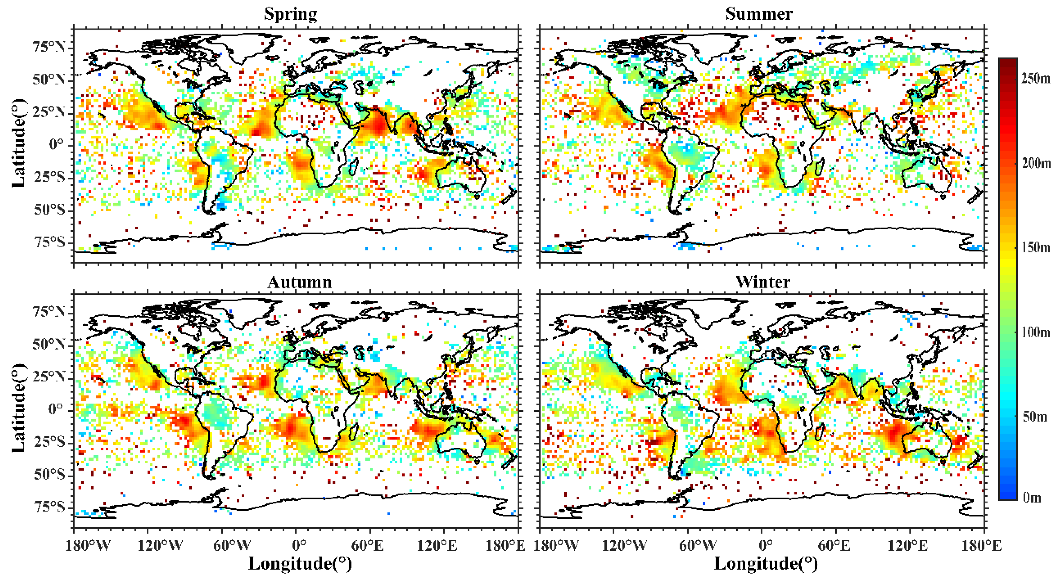
3.2. Altitude of Trapping

The trapping layer altitude $h_t$, has an important influence on the propagation of radio waves. Taking the average value of the trapping layer altitude in each grid, the seasonal distribution of the trapping layer altitude is shown in Figure 7.

The average altitude of the trapping layer is lower near the coast of the mainland than on the sea. This phenomenon can also be seen in Engeln’s results. With the distance away from the coastline, the altitude increases, such as is seen on the west coast of North America and the west coast of Africa. Similar situations also exist in continental seas, such as the Mediterranean Sea, the Persian Gulf, the Gulf of Aden, and the Red Sea [36]. The trapping layer on the land is mainly caused by radiative cooling, which mostly occurs on the surface or at low altitude [38]. Therefore, the trapping layer altitude is usually close to the land. As the distance into the sea increases, the temperature inversion gradually weakens, and the layer’s altitude gradually increases [11,39]. The emergence of the trapping layer is due to the sharp gradient of humidity and temperature related to the PBL stratocumulus, and the increasing altitude of the trapping layer away from the west coastline is related to the trade wind cumulus [8]. On account of being near the equator in the Southern Hemisphere, the northwest sea area of Australia in winter, under the control of tropical depression and the strong water vapor in the updraft, it is easy for stratocumulus to form in the air, thus producing a higher trapping layer. In summer, controlled by high pressure, the trapping layer is mainly caused by subsidence inversion. Therefore, the trapping layer occurrence rate, range and altitudes are lower. One point of concern is that areas with the larger trapping layer altitudes begin to shift southward in the Southern Hemisphere in autumn and winter.

The local time distribution of the average trapping layer altitude is shown in Figure 8. From the analysis of the diurnal changes in altitude, it can be seen that the altitude of the trapping layer is much higher in the daytime on the ocean than at night on the land. At LT00, most of the land trapping layer altitude is less than 300 m. During the day, solar radiation produces dry convective motion, which leads to the growth of the boundary layer. Trapping layers at altitudes of more than 1.3 km mainly occur in areas with a high occurrence rate, such as western Mexico and the south of America.

3.3. Intensity of Trapping

The trapping layer intensity refers to the difference in modified refractivity when the gradient$\mathrm{dM}/\mathrm{dh}<0$. As shown in Figure 1, the modified refractivity value corresponding to the top of the trapping layer ${\mathrm{h}}_{\mathrm{t}}$ is ${\mathrm{a}}_{\mathrm{s}}$, and the modified refractivity value corresponding to the bottom of the trapping layer ${\mathrm{h}}_{\mathrm{m}}$ is ${\mathrm{a}}_{\mathrm{m}}$. The value of ${\mathrm{a}}_{\mathrm{m}}-{\mathrm{a}}_{\mathrm{s}}$ is the intensity of the trapping layer. The greater the trapping layer intensity is, the greater the influence on radio wave propagation is.

According to the seasonal division, the average value of the trapping layer intensity in each grid point of latitude and longitude is taken to obtain the seasonal distribution of the trapping layer intensity in Figure 9. The intensity of the trapping layer on land is mostly between 0 M-unit and 15 M-unit, which is generally lower than that of the sea.

The trapping layer in the regions with a high occurrence rate usually has stronger intensity. In the eastern areas of oceans, the western coasts of continents and the Arabian Sea, and the northwest of Australia all illustrate this feature well. In the Arabian Sea, the occurrence rate and ranges of the trapping layer are the highest in spring, where a large-scale trapping layer intensity >30 M-unit appears. However, when this area is affected by the summer monsoon, the intensity reduces to 13~20 M-unit. In northwestern Australia, under the influence of the local pressure system, areas with intensity greater than 20 M-unit are more common in autumn and winter than in the other two seasons. Compared with the northwest and southwest regions of Africa, the intensity of the trapping layer in the northwest is over 24 M-unit in spring and summer, which is stronger than that in autumn and winter. In southwest Africa, on the other hand, it is stronger in autumn and winter than in spring and summer.

As it is affected by the intertropical convergence zone, the Northern Hemisphere has more areas with a stronger trapping layer in spring and summer than the Southern Hemisphere. In autumn and winter, the situation is reversed with the southward shift of the intertropical convergence zone.

Figure 10 shows the local time distribution of the trapping layer intensity. The intensity in most areas does not exceed 12 M-unit, and in areas with high occurrence rates, the intensity of the trapping layer is above 20 M-unit. The trapping layer intensity in the Arabian Sea reached the maximum value of 45 M-unit in LT18. The emergence of this strong trapping layer is mainly related to the increase in the temperature gradient and the humidity gradient, both of which are affected by solar radiation and sea–land breezes.

3.4. Thickness of Trapping

The occurrence rate of the trapping layer is closely related to the inversion layers [40]. Several studies of the PBL have already found that the inversion thickness at the top of the PBL varies between about 100 and 400 m [41]. Figure 11 shows the average thickness of the trapping layer in each season. The results show that the average thickness varies from 80 to 240 m. The thickness on land is smaller than that over the ocean, usually below 120 m.

The thickness is larger in the regions with a high occurrence rate of the trapping layer, too. The Arabian Sea has the most obvious seasonal variation, with the thickness exceeding 220 m in spring. Under the impact of the southwest monsoon in summer, the thickness decreases to about 100 m before increasing again in autumn and winter. In Australia, the thickness is obviously larger in autumn and winter than in spring and summer. These changes are consistent with the variation of the occurrence rate.

The trapping layer thickness on the northwest coast of Africa tends to shift northward in summer, and the thickness saw little overall variation; the average thickness is around 200 m. A large-scale lower trapping layer thickness appears over the Asian continent in summer, mainly due to the surface temperature inversion caused by radiative cooling.

In general, the trapping layer thickness seasonal variation is not significant; only a few areas have obvious changes. In spring and summer, the thickness of the Northern Hemisphere is greater than that of the Southern Hemisphere, but the opposite is true in autumn and winter.

The local time variations distribution of the trapping layer thickness is shown in Figure 12. Large areas of the trapping layer with an average thickness of more than 210 m appeared in the western sea areas of South America at LT12, and the average thickness in this area was between 150 m and 180 m at other times. The thickness of the areas in the northwest of Australia are higher in the daytime than at night, while the thickness of the central and northern African continent is greater at LT18 than at LT06. The local time variations of the trapping layer’s thickness in other regions are not obvious

4. Conclusions

We have used many years of historical occultation observation data and post-processing data to analyze and study the temporal and spatial distribution characteristics of the occurrence probability, altitude, intensity, and thickness of the trapping layer. The following conclusions can be drawn:

In general, the regions with high occurrence rates of the trapping layer are mainly concentrated in the eastern areas of the ocean and the western areas of the continents between 50° S and 50° N. Among them, the western oceans of Mexico, the western coast of Africa, the Arabian Sea, Red Sea, Mediterranean Sea and the sea areas of northwest Australia have a more than 50% occurrence rate of the trapping layer. The high trapping layer occurrence rate usually corresponds to relatively large altitude, intensity, and thickness.

There are geographical and seasonal differences in the distribution of the trapping layer characteristics in the Northern and Southern Hemispheres. The altitude, intensity and thickness of the trapping layer over the ocean are greater than that over the land. Generally, the altitude of the trapping layer is lower in the boundary areas between the oceans and the continents. The increased altitude of the trapping layer away from the western coastline is related to the trade wind cumulus. In spring and summer, the occurrence rate and range of the trapping layer in the Northern Hemisphere are higher than those in the Southern Hemisphere, but in autumn and winter, there are more occurrences in Southern Hemisphere than in the Northern Hemisphere.

The geographical and seasonal differences in the distribution of the trapping layer are affected by many climatic factors. Climatology shows that the areas with high occurrence rates of the trapping layers in western Mexico, the coastal areas of western Africa, the Red Sea, the Arabian Sea, the Mediterranean, and the Bay of Bengal are mainly affected by trade wind cumulus, ocean currents, equatorial convergence zone deviation, radiative cooling and other factors.

The diurnal variation of the occurrence rate, altitude, intensity and thickness is not obvious except for in a few areas. The main reasons for daily changes can be roughly divided into the following categories: firstly, boundary layer growth and boundary inversion caused by strong solar radiation heating; and secondly, boundary layer changes influenced by sea–land breezes.

References

1. Bean, B.R.; Dutton, E.J. Radio meteorology. In Technical Report Archive and Image Library; U.S. Government Publishing Office: Washington, DC, USA, 1966. [Google Scholar]
2. Kerr, D.E. Propagation of short radio waves (Revised edition). IEE Electromagn. Waves Ser. 1987, 24, 754. [Google Scholar]
3. Ao, C.O. Effect of ducting on radio occultation measurements: An assessment based on high-resolution radiosonde soundings. Radio Sci. 2007, 42, 1–15. [Google Scholar] [CrossRef] [Green Version]
4. Almond, T.; Clarke, J. Consideration of the usefulness of microwave propagation prediction methods on air-to-ground paths. In IEE Proceedings F (Communications, Radar and Signal Processing); IET Digital Library: London, UK, 1983; Volume 130, pp. 649–656. [Google Scholar]
5. Crane, R.K. Refraction. In Propagation Handbook for Wireless Communication System Design; CRC Press LLC: Boca Raton, FL, USA, 2003. [Google Scholar]
6. Turton, J.D.; Bennets, D.A.; Farmer, S.F.G. An introduction to radio ducting. Meteorol. Mag. 1988, 117, 245–254. [Google Scholar]
7. Engeln, A.V.; Nedoluha, G.; Teixeira, J. An analysis of the frequency and distribution of ducting events in simulated radio occultation measurements based on ECMWF fields. J. Geophys. Res. Atmos. 2003, 108. [Google Scholar] [CrossRef] [Green Version]
8. Engeln, V. A ducting climatology derived from the European Centre for Medium-Range Weather Forecasts global analysis fields. J. Geophys. Res. 2004, 109, 159–172. [Google Scholar] [CrossRef]
9. Basha, G.; Ratnam, M.V.; Manjula, G. Anomalous propagation conditions observed over a tropical station using high-resolution GPS radiosonde observations. Radio Sci. 2013, 48, 42–49. [Google Scholar] [CrossRef]
10. Saleem, M.U. Atmospheric Ducts Their Applications in Radio Frequency Propagation Using Satellite Remote Sensing Techniques Saarbrücken, 1st ed.; LAMBERT Academic Publishing: Sunnyvale, Germany, 2015; pp. 1–57. [Google Scholar]
11. Klein, S.A.; Hartmann, D.L. The seasonal cycle of low stratiform clouds. J. Clim. 1993, 6, 1587–1606. [Google Scholar] [CrossRef] [Green Version]
12. Duynkerke, P. Intercomparison of three- and one-dimensionalmodel simulations and aircraft observations of stratocumulus. Bound.-Layer Meteorol. 1999, 92, 453–487. [Google Scholar] [CrossRef]
13. Teixeira, J. Simulation of fog with the ECMWF prognostic cloud Scheme. Q. J. R. Meteorol. Soc. 1999, 125, 529–552. [Google Scholar] [CrossRef]
14. Tomczak, M.; Godfrey, J. Regional Oceanography: An Introduction; Daya Publishing House: Delhi, India, 2005; Volume 2. [Google Scholar] [CrossRef]
15. Kursinski, E.R.; Hajj, G.A.; Schofield, J.T. Observing Earth’s atmosphere with radio occultation measurements using the Global Positioning System. J. Geophys. Res. Atmos. 1997, 102, 23429–23465. [Google Scholar] [CrossRef]
16. Ware, R.; Rocken, C.; Solheim, F. GPS Sounding of the Atmosphere from Low Earth Orbit: Preliminary Results. Bull. Am. Meteorol. Soc. 1996, 77, 19–40. [Google Scholar] [CrossRef] [Green Version]
17. Wickert, J.; Reigber, C.; Beyerle, G. Atmosphere sounding by GPS radio occultation: First results from CHAMP. Geophys. Res. Lett. 2001, 28, 3263–3266. [Google Scholar] [CrossRef] [Green Version]
18. Hajj, G.A. CHAMP and SAC-C atmospheric occultation results and intercomparisons. J. Geophys. Res. 2004, 109. [Google Scholar] [CrossRef]
19. Anthes, R.; Ector, C.; Hunt, D.C. The COSMIC/FORMOSAT-3 mission early results. Bull. Am. Meteorol. Soc. 2008, 3, 313–334. [Google Scholar] [CrossRef]
20. Rocken, C.; Kuo, Y.H.; Scheriner, W.S. COSMIC System Description. Terr. Atmos. Ocean. Sci. 2000, 11, 21–52. [Google Scholar] [CrossRef] [Green Version]
21. Anthes, R.A.; Rocken, C.; Kuo, Y.H. Applications of COSMIC to Meteorology and Climate. Terr. Atmos. Ocean. Sci. 2000, 11, 115–156. [Google Scholar] [CrossRef] [Green Version]
22. Xie, F.; Wu, D.; Ao, C.O. Super-refraction effects on GPS radio occultation refractivity in marine boundary layers. Geophys. Res. Lett. 2010, 37, 174–187. [Google Scholar] [CrossRef]
23. Xu, X.; Luo, J.; Chuang, S. Comparison of COSMIC Radio Occultation Refractivity Profiles with Radiosonde Measurements. Adv. Atmos. Sci. 2009, 26, 1137–1145. [Google Scholar] [CrossRef]
24. ITU-R Rec. P.453-12. The Radio Refractive Index: Its Formula and Refractivity Data; International Telecommunication Union: Geneva, Switzerland, 2016. [Google Scholar]
25. Hitney, H.V.; Richter, J.H.; Pappert, R.A. Tropospheric radio propagation assessment. Proc. IEEE 1985, 3, 265–283. [Google Scholar] [CrossRef]
26. Zou, X.; Zeng, Z. A quality control procedure for GPS radio occultation data. Geophys. Res. 2006, 111. [Google Scholar] [CrossRef] [Green Version]
27. Sokolovskiy, S.V. Tracking tropospheric radio occultation signals from low Earth orbit. Radio Sci. 2001, 36, 483–498. [Google Scholar] [CrossRef] [Green Version]
28. Ao, C.O. Lower troposphere refractivity bias in GPS occultation retrievals. J. Geophys. Res. Atmos. 2003, 108, 4577. [Google Scholar] [CrossRef] [Green Version]
29. Beyerle, G.; Gorbunov, M.E.; Ao, C.O. Simulation studies of GPS radio occultation measurements. Radio Sci. 2003, 38, 1084. [Google Scholar] [CrossRef] [Green Version]
30. Xie, F.; Syndergaard, S.; Kursinski, E.R. An Approach for Retrieving Marine Boundary Layer Refractivity from GPS Occultation Data in the Presence of Super-refraction. J. Atmos. Ocean. Technol. 2006, 23, 1629. [Google Scholar] [CrossRef]
31. Rocken, C.; Anthes, R.; Exner, M. Analysis and validation of GPS/MET data in the neutral atmosphere. J. Geophys. Res. Atmos. 1997, 1022, 29849–29866. [Google Scholar] [CrossRef]
32. Marquardt, C.K.; Schöllhammer, K.; Beyerle, G. Validation and data quality of CHAMP radio occultation data. In First Champ Mission Results for Gravity Magnetic and Atmospheric Studies; Springer: Berlin/Heidelberg, Germany, 2003; pp. 384–396. [Google Scholar] [CrossRef]
33. Sokolovskiy, S. Effect of super-refraction on inversions of radio occultation signals in the lower troposphere. Radio Sci. 2003, 38, 1058. [Google Scholar] [CrossRef] [Green Version]
34. Ao, C.O.; Hajj, G.; Meehan, T.K. Rising and Setting GPS Occultations by Use of Open-Loop Tracking. J. Geophys. Res. Atmos. 2009, 114. [Google Scholar] [CrossRef] [Green Version]
35. Gossard, E.E.; Strauch, R.G. Radar Observation of Clear Air and Cloud. J. R. Meteorol. Soc. 1983, 110, 283–284. [Google Scholar]
36. Lopez, P. A 5-yr 40-km-Resolution Global Climatology of Super-refraction for Ground-Based Weather Radars. J. Appl. Meteorol. Climatol. 2008, 999, 89–110. [Google Scholar] [CrossRef]
37. Steele, J.; Thorpe, S.; Turekian, K. Ocean Currents; Academic Press: Cambridge, MA, USA, 2010. [Google Scholar]
38. Zhu, M.; Atkinson, B.W. Simulated Climatology of Atmospheric Ducts over the Persian Gulf. Bound.-Layer Meteorol. 2005, 115, 433–452. [Google Scholar] [CrossRef]
39. Teixeira, J.; Hogan, T.F. Boundary Layer Clouds in a Global Atmospheric Model: Simple Cloud Cover Parameterizations. J. Clim. 2001, 15, 1261–1276. [Google Scholar] [CrossRef]
40. Cheng, Y.H. Observed characteristics of atmospheric ducts over the South China Sea in autumn. Chin. J. Oceanol. Limnol. 2015, 34, 619–628. [Google Scholar] [CrossRef]
41. Siebesma, A.P.; Bretherton, C.S.; Brown, A. A large eddy simulation intercomparison study of shallow cumulus convection. J. Atmos. Sci. 2003, 60, 1201–1219. [Google Scholar] [CrossRef]
Figure 1. Schematic illustration of trapping layer and duct.
Remotesensing 13 03839 g001
Figure 2. A comparative example of refractivity data before and after cubic spline interpolation.
Remotesensing 13 03839 g002
Figure 3. The global distribution of the data count within the 2_deg by 2_deg grid.
Remotesensing 13 03839 g003
Figure 4. The number of the trapping layer concurrences within the 2_deg by 2_deg grid.
Remotesensing 13 03839 g004
Figure 5. Distribution of the trapping layer occurrence rate with season variations. The blank grids represent that there is no radio occultation event.
Remotesensing 13 03839 g005
Figure 6. Distribution of the trapping layer occurrence rate with local time variations. The blank grids represent that there is no radio occultation event.
Remotesensing 13 03839 g006
Figure 7. Distribution of the trapping layer altitude with season variations. The blank grids represent that there is no trapping layer event.
Remotesensing 13 03839 g007
Figure 8. Distribution of the trapping layer altitude with local time variations. The blank grids represent that there is no trapping layer event.
Remotesensing 13 03839 g008
Figure 9. Distribution of the trapping layer intensity with season variations. The blank grids represent that there is no trapping layer event.
Remotesensing 13 03839 g009
Figure 10. Distribution of the trapping layer intensity with local time variations. The blank grids represent that there is no trapping layer event.
Remotesensing 13 03839 g010
Figure 11. Distribution of the trapping layer thickness with season variations. The blank grids represent that there is no trapping layer event.
Remotesensing 13 03839 g011
Figure 12. Distribution of the trapping layer thickness with local time variations. The blank grids represent that there is no trapping layer event.
Remotesensing 13 03839 g012