Abstract
Harvester-mounted yield monitor sensors are expensive and require calibration and data cleaning. Therefore, we evaluated six vegetation indices (VI) from unmanned aerial system (Quantix™ Mapper) imagery for corn (Zea mays L.) yield prediction. A field trial was conducted with N sidedress treatments applied at four growth stages (V4, V6, V8, or V10) compared against zero-N and N-rich controls. Normalized difference vegetation index (NDVI) and enhanced vegetation index 2 (EVI2), based on flights at R4, resulted in the most accurate yield estimations, as long as sidedressing was performed before V6. Yield estimations based on earlier flights were less accurate. Estimations were most accurate when imagery from both N-rich and zero-N control plots were included, but elimination of the zero-N data only slightly reduced the accuracy. Use of a ratio approach (VITrt/VIN-rich and YieldTrt/YieldN-rich) enables the extension of findings across fields and only slightly reduced the model performance. Finally, a smaller plot size (9 or 75 m2 compared to 150 m2) resulted in a slightly reduced model performance. We concluded that accurate yield estimates can be obtained using NDVI and EVI2, as long as there is an N-rich strip in the field, sidedressing is performed prior to V6, and sensing takes place at R3 or R4.
1. Introduction
Corn (Zea mays L.) grain yield is an important measure for farmers to evaluate field management [1]. Yield can be measured at different scales, such as county-scale, field-scale, and within-field-scale, and each scale is useful for different management approaches. Yield monitor systems installed on grain combines have been used for over 25 years [2] and typically record yield at 1 s intervals. The data can be transformed into maps that can be used to identify low- and high-performing areas within a field and manage them appropriately. However, yield monitor systems are expensive, require field calibration, and often contain errors that have to be eliminated in a data cleaning process before the data can become actionable [2,3]. Furthermore, yield monitor systems can only collect data at the time of harvest (destructive approach), which means measurements can be performed only once. Therefore, there is a need for a simple, accessible, and nondestructive approach to estimate yield at the within-field scale that can operationally be used by many farmers. Remote sensing, via unmanned aerial systems (UASs) and/or traditional airborne/spaceborne platforms, offers one potential solution.
Advancements in remote sensing platforms, including the use of UASs equipped with multispectral sensors, now allow for within-field yield estimation, which in turn can be managed to improve overall farm productivity [4,5]. Sensors onboard UASs are typically passive sensors, i.e., sensors that capture electromagnetic energy emanating from an independent source and reflecting from of a crop/soil (depending on field coverage driven by growth stage of the crop). Such spectral imagery can then be used to calculate vegetation indices (VIs) that are correlated to crop status and biomass. For example, the near-infrared (NIR) band of a multispectral sensor can detect organic compounds present in living tissue, which can be used to identify stressed plants [6].
Most of the VIs used in agriculture today utilize NIR-band information. The most common VI is the normalized difference vegetation index [NDVI], calculated using NIR- and red-band reflectance and developed by [7]; this index has subsequently been used even in recent studies [8,9,10,11,12]. Several other indices are also used in agriculture for estimating yield, such as the excess green index (EXG), enhanced vegetation index-2 [EVI2], simple ratio index [SR], green normalized difference vegetation index [GNDVI], and triangular greenness index [TGI] [13,14,15,16,17]. Among these indices, NDVI, GNDVI, EVI2, and EXG have been used for vegetation mapping, biomass estimation, and the yield estimation of different crops, while the other two indices, SR and TGI, represent recently reported indices that could be well-suited for yield estimations [13,16].
Yield estimation models typically correlate VIs (predictor variables) from the remotely sensed imagery with yield data (response variable), obtained from harvester-mounted yield monitor systems [3,17,18]. Some studies have treated yield data as categorical. For example, some researchers have classified yield into three and five classes [19,20], achieving prediction accuracies greater than 70%. Other studies have treated yield as a continuous numerical variable, modeled against VIs using regression approaches, with R2 values ranging between 0.33 and 0.74 [3,8,11,12,21]. While some studies have used linear regression models for yield estimation [17,21,22], exponential regression models [8,11,12] are more commonly used.
It is well-established that the NDVI can be used for in-season N management; typically, N-deficient portions of a field, sensed between V7 and VT, will exhibit lower NDVI values than areas in the field that are not N-limited [23,24]. However, the timing of sensing is important, with better estimates obtained when sensing is performed later in the season [8,12,21]. A study by [8], which combined the timing of N sidedress applications (V4, V6, V8, and V10) with the timing of sensing NDVI, showed that delaying sensing until R2 resulted in a better accuracy (R2 > 0.80) than assessment earlier in the season. This study also showed that the delaying of sidedressing impacted not only the yield, but also the ability to accurately estimate the yield from NDVI signals. Additionally, previous studies have concluded that for the most accurate yield estimation from NDVI signals, an N-rich treatment (excess N applied at planting) is needed for the calibration of reflectance signals [11,25]. Many studies have also included signals from zero-N treatments, where no additional N is applied beyond possibly a small starter N application.
Sensing should be performed early enough for management intervention, but late enough to allow for assessment of the N status of a crop, when NDVI is used to determine whether additional N is needed for a crop. This is typically best-performed between V6/V7 [12] and V12 [8]. Beyond these growth stages, plant size imposes restrictions on the sensing of the crop canopy and the addition of N may be too late to recover a truly deficient crop. However, when sensing crops for yield estimation with UAS-mounted sensors or satellite platforms, sensing can be performed later. This allows for more accurate yield estimations, as reported in studies such as [16], which showed accurate estimates with sensing at R1 [8], where R2 exhibited better results than earlier in the season, and [15], which showed sensing between R4 and R6 to be optimal. These studies showed the potential of using remotely sensed data for accurately estimating yield early in the growing season, which is a definite advantage over the use of yield monitors mounted on the harvester, which collect data at harvest only.
More research is needed to evaluate VIs for their ability to estimate corn grain yield from UAS-mounted sensors, with attention to field management (timing of sidedressing), reference checks (zero-N and N-rich controls), and timing of sensing (vegetative versus reproductive growth stages). The specific objectives of this study were thus to: (i) compare various vegetation indices for their ability to estimate yield with sensing at the R4 growth stage; (ii) determine the effect of sidedress application timing on yield estimation from sensing data obtained at the R4 growth stage; (iii) estimate the performance of VI-based corn yield prediction models with earlier sensing times (V and early R stages); and (iv) evaluate whether the zero-N strip (control) is essential for deriving accurate yield estimation models. In addition to the evaluation of yield models derived directly from VI values, we also evaluated a ratio approach, where the VI relative to VI of the N-rich treatments is used to derive relative yield (yield compared with yield in the N-rich treatment), with and without the inclusion of VI values from zero-N control treatments in the models. Finally, we evaluated the effect of sampling area (plot size) on accuracy of the most promising yield estimation models.
2. Materials and Methods
2.1. Experimental Research Plot
The experiment was conducted during the growing season of 2019 at the Musgrave Research Farm, Aurora, NY, USA (42.732513 N, 76.658823 W). The experimental area was 1.1 ha (2.65 acres), with original plot dimensions of 110 m × 95 m. Soil types included Lima silt loam (61%) and Honeoye silt loam (39%). Further details about the soil, such as pH, organic matter, and extractable P, have been detailed in a previous study [8]. Corn (Pioneer P9188AMXT) was planted at a seeding rate of 79,000 seeds ha−1 on 27 May 2019, using a row spacing of 0.76 m and a small starter application of 224 kg of 10-20-20 (N-P2O5-K2O) with 1% Zn, which supplied 33 kg N ha−1 to all plots. The corn variety and the planting specifications were selected to be consistent with variety use on a neighboring farm. Corn was harvested for grain on 19 November 2019.
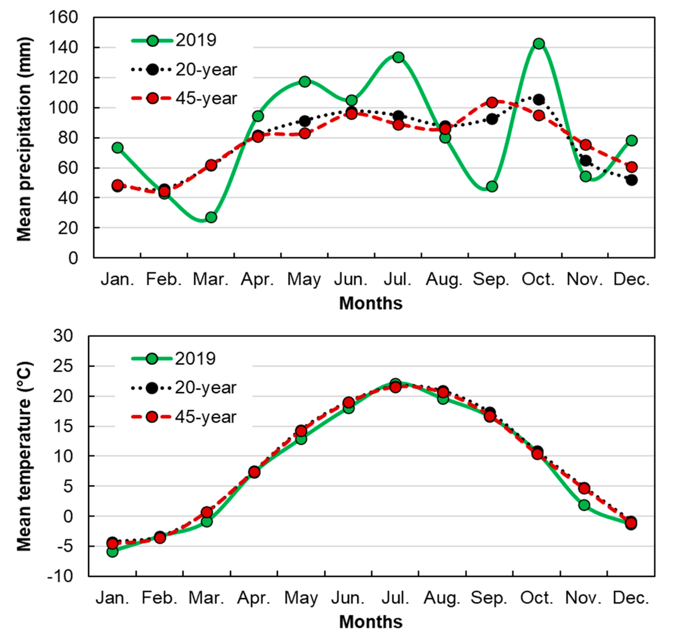
Monthly precipitation data were accessed from CLIMOD2 [26]. The cumulative precipitation recorded in 2019 at this location between May and November was 685 mm, with a monthly average of 98 mm (Figure 1). May and June received 117 and 105 mm, respectively, which were highly favorable for initial corn growth. Compared to the precipitation of 2018 reported earlier [8], precipitation was optimal for the growing season.
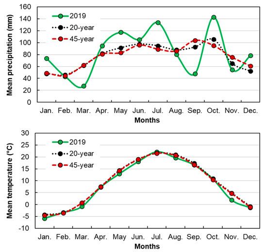
Figure 1.
Mean precipitation and temperature during 2019 corn growing season along with 20-year and 45-year average. Weather data retrieved from the station at the Musgrave Research Farm in Aurora, New York from CLIMOD2.
2.2. Sidedress N treatments Application
A randomized complete block design (RCBD) was employed with six treatments and three replications. Each treatment strip was 3 m wide and 95 m long (edge-to-edge), but for the analysis, only the center portion of the field was used, resulting in 3 m wide and 50 m long strips for each treatment (Figure 2).
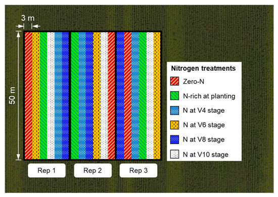
Figure 2.
Illustration of the experimental design and UAS data collection timing for N treatments conducted at the Musgrave Research Farm, Aurora, NY, USA. The base-map shown is the aerial imagery obtained at the R4 growth stage of corn on 22 August 2019. The zero-N treatment received starter N (33 kg N ha−1) only, the N-rich treatment received 336 kg N ha−1 before emergence, and all four sidedress treatments received 202 kg N ha−1 at their respective growth stages.
All N treatments were surface-applied using Agrotain-treated urea (Koch Agronomic Services, LLC, Wichita, KS). Six different N treatments included a zero-N (control), an N-rich treatment (336 kg N ha−1 at planting), and sidedress N application (202 kg N ha−1) applied at V4, V6, V8, or V10. The N-rich treatment was applied prior to emergence (8 days after planting).
2.3. Unmanned Aerial System (UAS) Image Acquisition
Aerial images were acquired using a UAS, QuantixTM Mapper supported by the AeroVironment Decision Support System (AV DSSTM, AeroVironment Inc., Arlington, VA, USA). The UAS was operated using a Quantix Mapper operating tablet supplied by the company. The tablet was equipped with an inbuilt application for mission planning and control. Once the field boundary was delineated in the application, an optimized flight path with parallel passes was automatically generated. The field boundary and flight mission plans were set-up during the first flight and consistently followed for subsequent dates. This ensured that all the images obtained were georeferenced to the same boundary points in the field. The front and side overlaps were consistently maintained at 85% and 60%, respectively, to ensure seamless stitching. The image capture rate was automatically adjusted in the application to maintain overlap.
The UAS was equipped with an RGB camera with red (583–673 nm), green (506–586 nm), and blue (415–500 nm) bands, and a multispectral camera with red (581–657 nm), green (533–604 nm), and near-infrared (NIR; 795–884 nm) bands. Both cameras captured images at nadir and the image dimensions were 4864 × 3648 pixels and 2432 × 1824 pixels, respectively. The RGB and multispectral camera used a self-calibrating downwelling solar sensor that measures ambient light to calibrate each band.
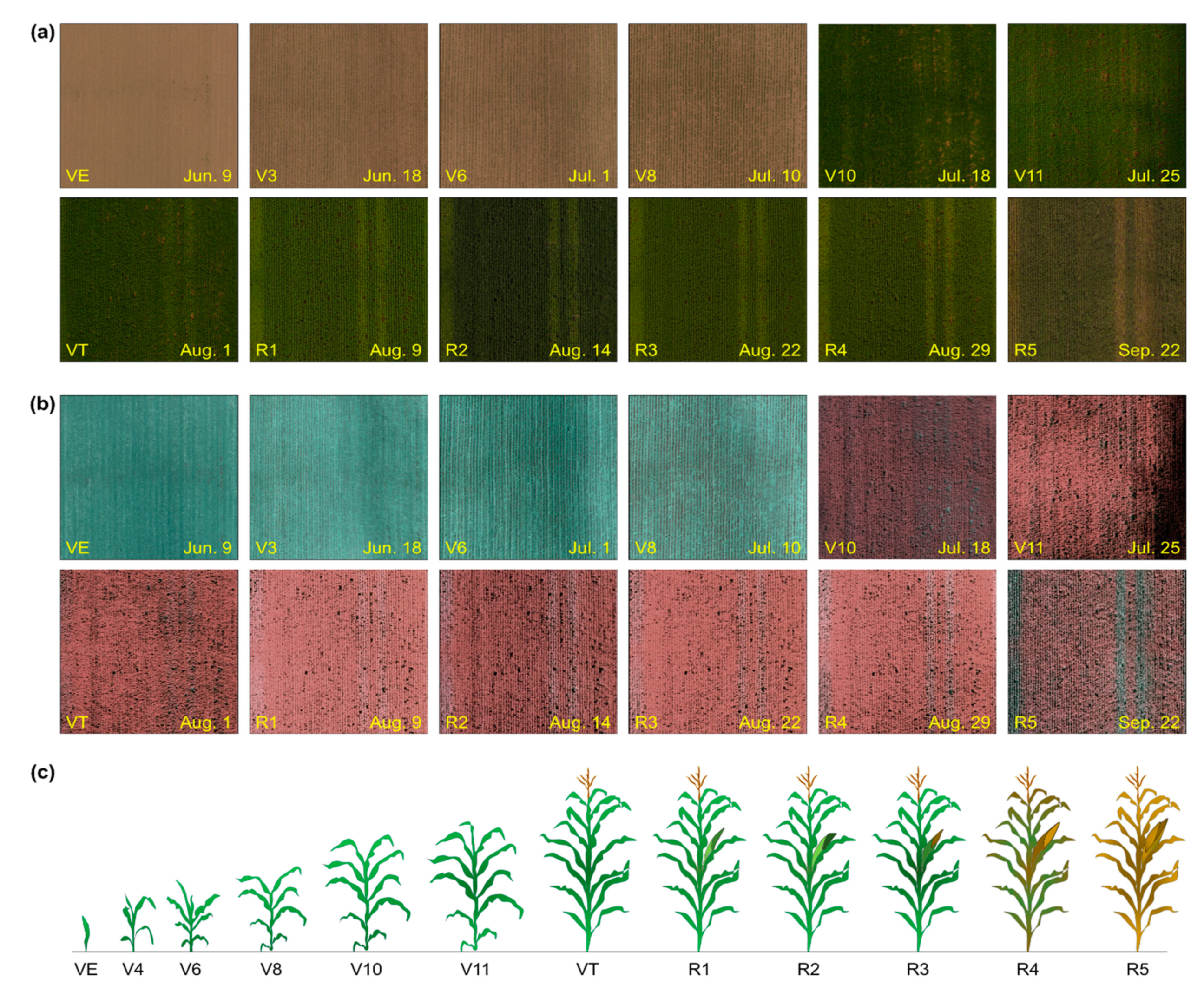
Flights were performed for each growth stage, starting from the corn emergence stage (VE) until the kernel dent stage (R5) (Figure 3). All the flights were made between 9 and 11 AM, which was found to be the best time for yield estimations from our previous study [8]. The UAS was flown at an altitude of ~110 m (361 ft.) above ground level, resulting in a ground sampling distance (GSD) of 2.5 cm/pixel (1 inch/pixel) for the RGB and 5.0 cm/pixel (2 inch/pixel) for the multispectral imagery. The images were uploaded to the cloud AV-DSS platform to obtain orthomosaiced (stitched) images and for canopy cover estimation. The image stitching service was also provided by the AV-DSS platform.
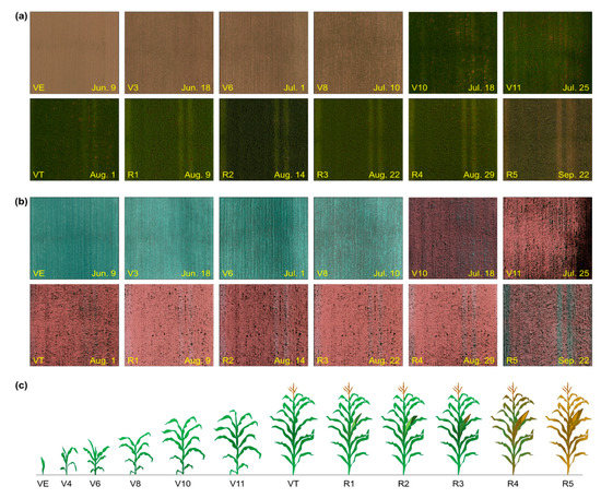
Figure 3.
(a) Color imagery obtained using the RGB camera from a Quantix hybrid drone at different corn growth stages, from VE to R5; (b) false-color composite imagery obtained from the multispectral sensor, visualized by arranging the NIR-red-green layers as an R-G-B display; and (c) schematic representation of corn growth stages from VE to R5.
2.4. Corn Grain Yield Data Collection and Cleaning
Corn grain was harvested using a Case IH 2144 combine equipped with an AgLeader InCommand 800 yield monitor system. The combine had a AgLeader GPS 6500 receiver unit, which has a horizontal position accuracy of 0.4 m. The combine had a 4-row corn head (3 m swath width). Thus, per pass, one strip of harvest data was obtained. Yield monitor data were processed and cleaned following a semi-automated yield data cleaning protocol [27,28]. Kharel et al. [28] showed that implementation of their post-harvest data cleaning protocol was essential to obtaining accurate yield data for within-field management and on-farm trials.
2.5. Yield and Color Values Extraction for Each Treatment
A free, open-source geographic information system (GIS) software, QGIS 3.16.2 (Hannover), was used to extract the average yield values of each N treatment and associated spectral values from UAS imagery. Plots were subdivided in one of three ways in order to study the effect of size of sampling area (experimental unit): (1) each N treatment strip was considered as an experimental unit that resulted in a sampling area of 150 m2, with three data points per treatment (n = 3); (2) the whole N strip length was divided into two parts, resulting in a sampling area of 75 m2 with six data points per treatment (n = 6); and (3) a buffer polygon of 3 × 3 m was placed around each yield data point, which resulted in a sampling area of 9 m2 with 16 data points per treatment (n = 16).
The average yield value inside each treatment strip was obtained using the “join attributes by location (summary)” option in QGIS. Average band values from the UAS imagery (raster layer) were extracted using the “zonal statistics (summary)” option in QGIS. The yield and color values from weekly flights were exported to individual comma-separated-value (CSV) files and used for further analysis.
2.6. Vegetation Index Calculation
Six different vegetation indices were calculated using a user-coded program, developed in R statistical software [29]. Of the six indices, four vegetation indices used the NIR band commonly used in various yield estimation applications [13,16]. The other two common indices, i.e., EXG and TGI, were included to test if accurate yield estimations are possible with images obtained only from RGB bands. This would extend the possibility of using any basic UAS for yield estimation application. R code was used for calculating spectral VIs from CSV files:
where NDVI is the normalized difference vegetation index, GNDVI is the green normalized difference vegetation index, EVI2 is the two-band enhanced vegetation index, SR is the simple ratio, EXG is the excess green index, and TGI is the triangular greenness index. As the images were produced from two sensors at different image resolutions, images were not combined or overlapped for any of the above vegetation index calculations. The vegetation indices involving the NIR band (Equations (1)–(4)) were calculated from the multispectral imagery, while the other two indices (Equations (5) and (6)) were calculated from the RGB imagery only.
NDVI = (NIR − Red)/(NIR + Red)
GNDVI = (NIR − Green)/(NIR + Green)
EVI2 = (2.5 × (NIR − Red))/(NIR + 2.4 × Green + 1)
SR= NIR/Red
EXG = 2 × Green − Red − Blue
TGI = Green − 0.39 × Red − 0.61 × Blue
2.7. Yield Model Development
It has been shown that exponential models are best suited for yield estimation for corn grain in New York [8,12]. Such models are simplified as:
where a and b are fitted parameters. Models were developed in R statistical software. Eight different combinations of sidedress treatments were developed and tested: (i) Combination 1: zero-N + N-rich; (ii) Combination 2: zero-N + N-rich + V4; (iii) Combination 3: zero-N + N-rich + V6; (iv) Combination 4: zero-N + N-rich + V8; (v) Combination 5: zero-N + N-rich + V10; (vi) Combination 6: zero-N + N-rich + V4 + V6; (vii) Combination 7: zero-N + N-rich + V4 + V6 + V8; and (viii) Combination 8: zero-N + N-rich + V4 + V6 + V8 + V10. The reliability of the models was assessed based on the coefficient of determination (R2) with higher R2 indicating better reliability.
Yield= a × exp^(b×VI)
2.8. Data Analysis
Yield responses to different N sidedress treatments were evaluated via a linear mixed-effects model using the lme4 package [30] in R software. The mixed-effects model was used because it can simultaneously model fixed and random effects. The N sidedress treatment was considered a fixed effect and replication was considered a random effect. The idea of using N sidedress treatment as the fixed effect is because we expected the effects to persist across different N treatments, while the replication was considered as the random effect because the variation within each treatment group does exist based on the many other underlying parameters, which have to be suppressed. This model was performed using the R command: model = lme(Yield~Treatment, random =~1|replication). The mean comparison analysis was performed using the lsmeans package [31] with the R command: groups = lsmeans(model, ~Treatment). Six different vegetation indices were evaluated from the UAS imagery, obtained at the R4 growth stage, while model performance was evaluated based on R2 values. Reliable sidedress timing for accurate yield estimations was selected based on the fitted model performance. Yield models using data points from the eight sidedress combinations were tested to identify the best combination.
The selected vegetation indices from objective 1 from earlier flight dates (VE to R5) were used to construct yield estimation models, and their performance was evaluated to identify the best time/stage for sensing. The analysis was performed with and without the inclusion of results from the zero-N treatments, to test if the zero-N strip (control) can be eliminated.
To extend the usability of the models, we further scaled all the treatments by considering a ratio with respect to N-rich treatment, with and without inclusion of the zero-N treatment data. This scaling was performed for both yield and each vegetation index as follows:
where YieldTrt and VITrt are the yield and vegetation index values from each N treatment, respectively, and YieldN-rich and VIN-rich are the yield and vegetation index values from only the N-rich treatment. The models developed using the ratio VI values allows us to estimate relative yields that helps in identifying high and low yielding areas.
Lastly, we evaluated the effect of plot size on model performance using three different sampling areas, namely 150 m2, 75 m2, and 9 m2, by sectioning the treatment strip accordingly. The best models were validated via leave-one-out cross-validation and the estimated map was generated using a raster calculator with a 1 m/pixel spatial resolution.
3. Results and Discussion
3.1. Yield Response to Timing of N Sidedress Application
Yields within the same treatment varied from 3.8–6.9 Mg ha−1 for the zero-N control plots, to 8.6–12.4 Mg ha−1, 8.5–11.9 Mg ha−1, 9.3–12.2 Mg ha−1, 9.1–11.4 Mg ha−1, and 8.1–11.2 Mg ha−1 for the N-rich and sidedressing at V4, V6, V8, and V10 treatments, respectively. Delaying sidedressing beyond V6 reduced yield, consistent with findings from prior years at the same location [8].
The response index (ratio of yield of the N-rich treatment to yield at zero-N) was 2.0. This response index was identical to the index in 2015, but higher than the index of 1.3 obtained in 2016 at the same location [11], similar to the 2.2 index for a study in 2017, and lower than the 3.6 response index determined for 2018 [8]. Changes from year to year primarily reflect growing season weather differences, with lower indices for years with more challenging weather patterns, such an extremely wet spring, followed by a drought in 2016.
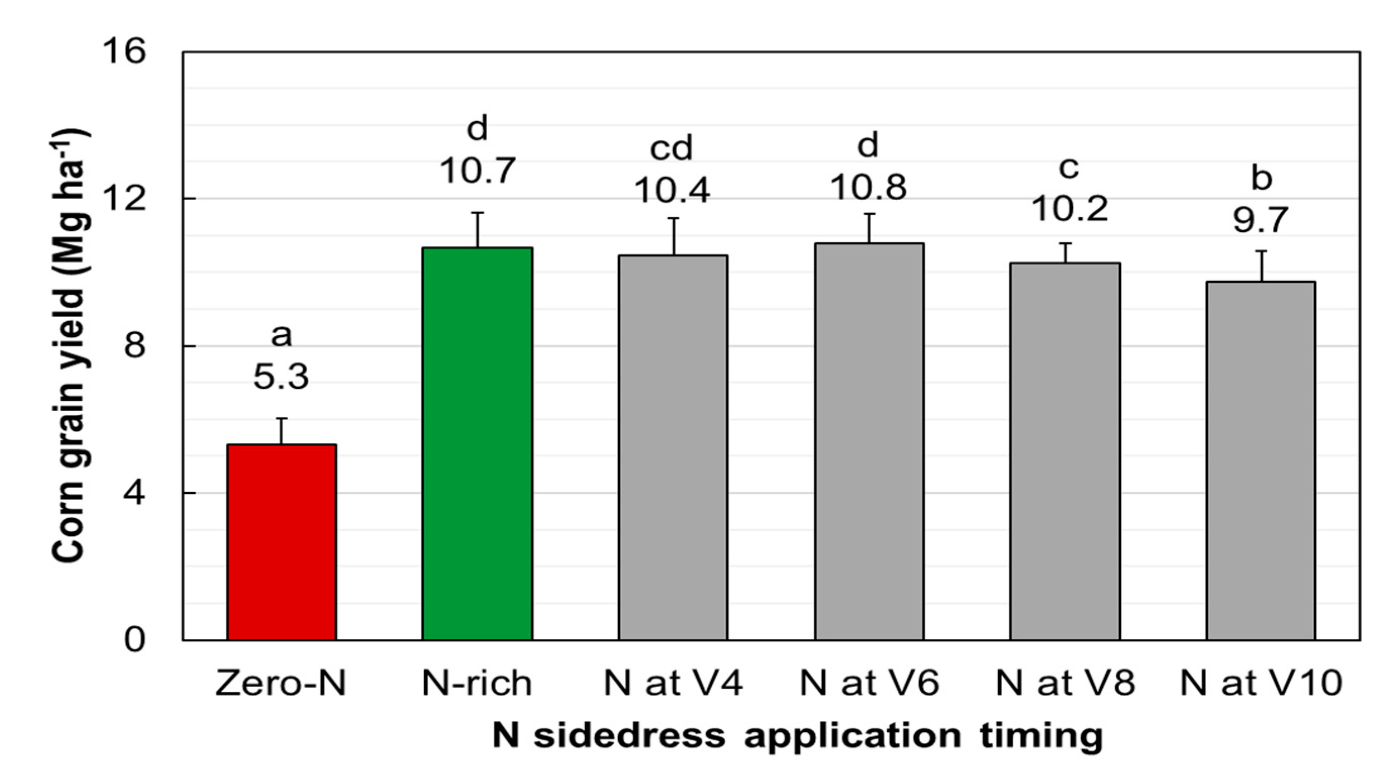
Sidedressing at V4 and V6 resulted in yields similar to those obtained with the N-rich treatment (Figure 4), even though only 60% of the N was applied for sidedressing. These findings are similar to those of [32], which reported that the yield was not impacted by sidedressing at V4 to V6 compared to an N-rich treatment, independent of the N application method. Sidedressing at V8 and V10 still increased the yield beyond the zero-N control but the yield averaged 95 and 91% of the yield obtained by N-rich treatment, respectively. The reduction in yield compared to the N-rich treatment is consistent with reductions observed during prior years, where the yield averaged 94% and 73% when sidedress was delayed to V8 and V10, respectively (Maresma et al. 2020). While a few studies reported no significant differences in the yield with delayed sidedressing [33,34,35], our results were expected, given the limited amount of N applied with the starter, and the absence of other N sources, such as a cover crop or manure.
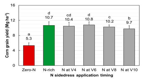
Figure 4.
Corn grain dry matter yield as affected by N sidedress application treatments. Zero-N received starter N (33 kg N ha−1) only, N-rich received 336 kg N ha−1 prior to emergence, and all other sidedress N treatments received 202 kg N ha−1 at different growth stages (V4–V10). The statistical labels stem from a mean comparison analysis using Tukey’s HSD (α = 0.05).
3.2. Vegetation Indices Selection for Estimating Yield
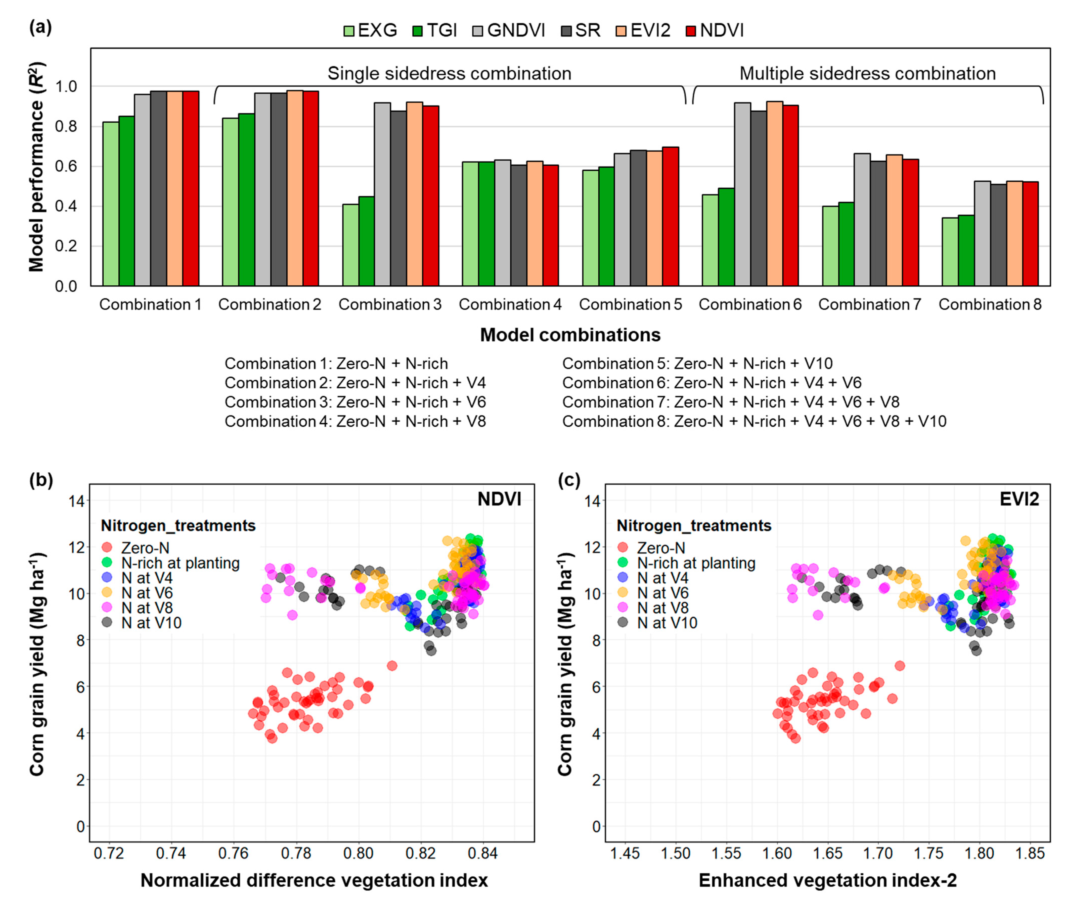
Among the six VIs evaluated as predictors for yield with flights at R4, four of them—NDVI, EVI2, SR, and GNDVI—performed similarly in all treatment combinations (Figure 5). The other two VIs—EXG and TGI—were consistently lower-performing. These two VIs were tested as low-cost RGB-based estimators of corn yield and N requirements [17,36], while the others included NIR (Equations (1)–(4)), which points to the importance of including NIR for the most accurate yield predictions. These findings are consistent with studies by [13,15] that attributed the better performance of GNDVI for corn yield estimations using UAS and satellite images to the inclusion of reflectance from green and NIR bands (Equation 2), which are more strongly correlated with leaf chlorophyll, N content, and grain yield than other bands are [13]. The results did show, however, that where the NIR band information was absent, EXG and TGI can be used to calibrate yield models, with R2 values ranging from 0.82 to 0.86, as long as sidedressing is performed at or before V4 (Figure 5a).
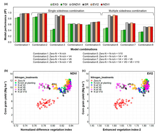
Figure 5.
(a) Model performances of six different vegetation indices, obtained from imagery captured at R4, for eight different sidedress treatment combinations, (b) relationship between the NDVI and yield data for each N treatment, and (c) relationship between EVI2 and yield data for each N treatment. Note: Zero-N received starter N (33 kg N ha−1) only, N-rich received 336 kg N ha−1 prior to emergence, and all other sidedress N treatments received 202 kg N ha−1 at different growth stages (V4–V10). The scatter plots (b,c) were only shown for selected vegetation indices as they were the top two reliable indices for yield estimation.
Among the top four performing indices, NDVI and EVI2 produced the highest R2 values. The performance of NDVI for estimating yield is consistent with previous studies at the same location [8,12]. EVI2 was used instead of EVI because the multispectral camera in the UAS did not provide blue channel information. In fact, the purpose of developing the EVI2 index was to use only two bands (NIR and red) for extracting further crop-related information from other remote sensing platforms [37]. Though the blue channel was available from the RGB camera, it could not be used for evaluating EVI, because it was calibrated separately. Previous studies have also demonstrated that EVI2 can be a good indicator of corn yield [14], and a few studies have reported that EVI2 is a better indicator than NDVI for estimating crop yield [38,39]. In this study, only NDVI and EVI2 were selected for further evaluation.
3.3. Reliable Sidedress Treatment Selection for Yield Estimation
Sidedress timing impacted the yield prediction model performance from imagery collected at R4. Predictions were most reliable when sidedressing took place at or before V6, while a delay in sidedressing beyond V6 resulted in considerably lower R2 values for yield estimation models derived from EVI2 and NDVI (Figure 5a). Models based on imagery from the zero-N and N-rich plots (combination 1) resulted in the highest R2, followed by a model based on data including plots sidedressed at V4 (combination 2) and those sidedressed at V6 (combination 3). The NDVI and yield data points were well-separated, forming independent groups of points when only zero-N and N-rich data points were fitted (Figure 5b,c). Although the inclusion of any N sidedress treatment beyond V6 resulted in higher NDVI values, as reported by [34], it produced scattered NDVI and EVI2 values (Figure 5b,c), which reduced the R2 values of the yield models. When multiple treatment combinations were used to derive yield estimates, only combination 6 (zero-N + N-rich + V4 + V6) reliably produced high R2 values of 0.92 and 0.90 for EVI2 and NDVI, respectively. All other combinations had lower R2 (<0.65). These results suggest that the N-rich treatment strip is important for yield estimation for fields responsive to N, consistent with findings by [11]. Based on these results, only the combinations that included sidedress up to V6 were selected for further evaluation (combinations with V8 and V10 were excluded).
3.4. Yield Estimations at Earlier Growth Stages
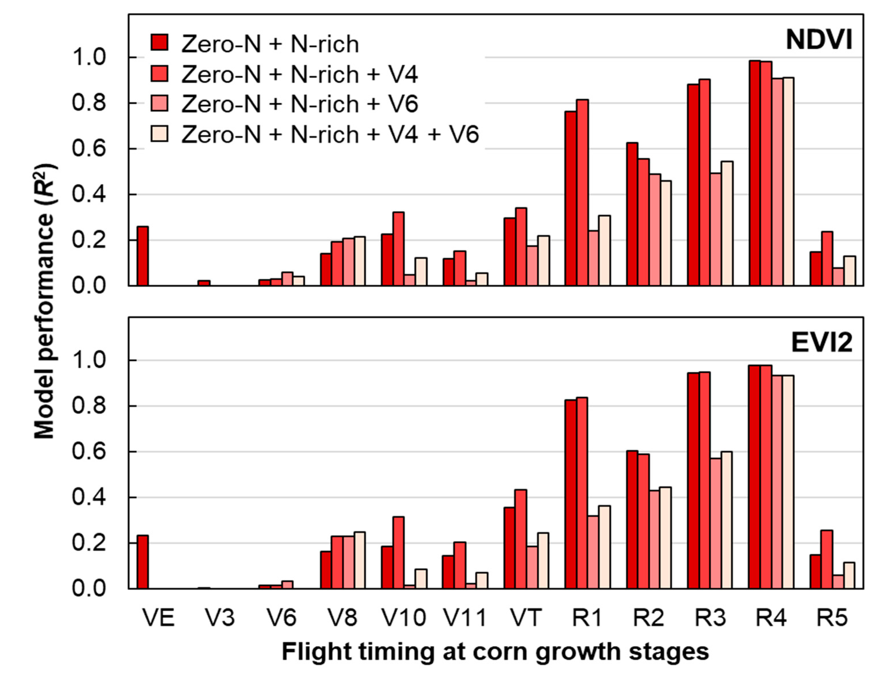
The NDVI and EVI2 data for each plot, along with four N sidedress combinations (1, 2, 3, and 6; excluding 4, 7, and 8) from earlier flight dates (VE to R5), were used to evaluate the best time/stage for image collection toward reliable yield estimations. The results indicate that sensing at R4 resulted in the most accurate models (Figure 6), consistent with other studies [15]. Though sensing earlier in the season allows for in-season crop management decisions, the findings here and results from other studies [12,21,40] show that yield estimates are considerably more reliable when sensing takes place after silking (R1).
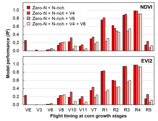
Figure 6.
Corn yield estimation model performance of selected vegetation indices and selected sidedress treatment combinations from the UAS images obtained throughout the growing season of 2019.
There was a drastic reduction in model performance with imagery collected at R5 (Figure 6). This reflected a yellowing of the crop canopy (Figure 3) that changed crop reflectance and made images collected at this growth stage unsuitable for yield estimation. These results are consistent with [23], which also noted a drastic reduction in performance of yield models when sensed at physiological maturity. The reduced R2 of models developed from imagery collected at R2 in our study was not expected and is inconsistent with previous work [8]. The reduction in performance in our study may be due to cloudy conditions at image acquisition, which can be observed with a slight darkening when comparing R1 and R3 in Figure 3a,b. This finding stresses the need for somewhat consistent illumination conditions during image acquisition, even given the downwelling sensor that allows for real-time calibration to reflectance.
The results indicate that for reliable yield estimates (R2 > 0.80), sensing should take place once reproductive stages have been reached, prior to senescence of the crop (R1–R4), while models should include imagery from zero-N and N-rich treatments, augmented by areas where sidedressing was performed at V4 at the latest. As stated above, flights ideally should occur on sunny days with limited cloud coverage.
3.5. Effect of Eliminating the Zero-N Treatment
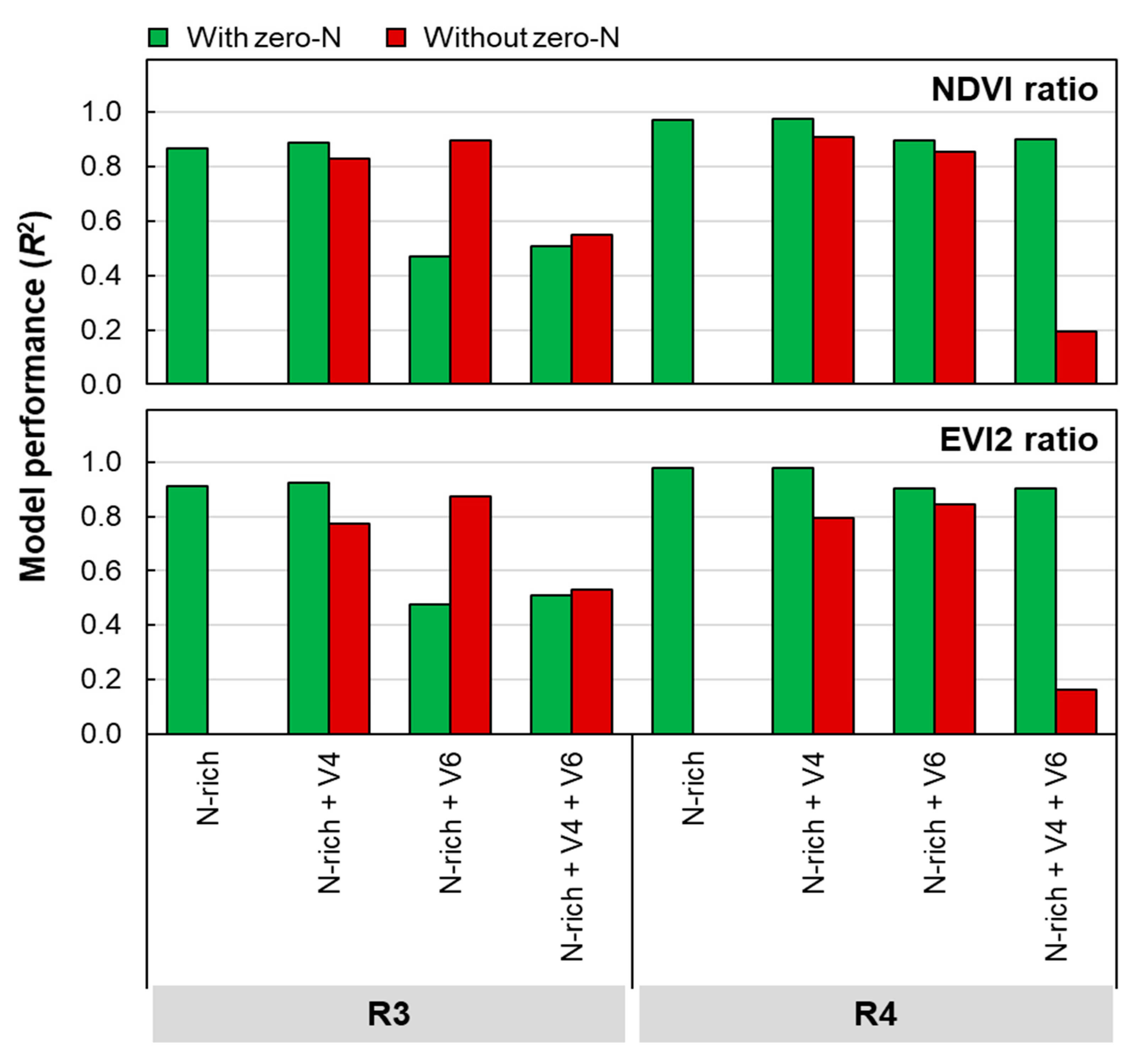
The zero-N treatment causes a significant yield reduction, as has been the case in other remote sensing studies [8,34]. While including the zero-N treatment resulted in more reliable models, excluding this treatment when developing models slightly reduced the R2 of the models (Figure 7), as long as sidedressing took place early (V4) and sensing was performed at R4. Models that included imagery from the plots sidedressed at V6 showed considerably lower R2 values. Models based on NDVI showed more stable performance without zero-N than models based on EVI2, perhaps reflecting the sensitivity of EVI2 in capturing subtle differences in vegetation. Such differences could have caused variability and likely be the reason for reduced R2 within treatments without zero-N.
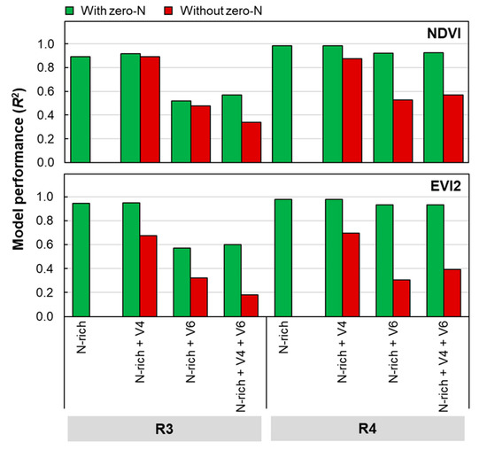
Figure 7.
Corn yield estimation model performance using NDVI and EVI2 as inputs and selected sidedress treatment combinations, with and without zero-N treatment (33 kg N ha−1 starter N only, no sidedress N application) included at R3 and R4.
3.6. Relative Yield Estimation Accuracies with and without Zero-N
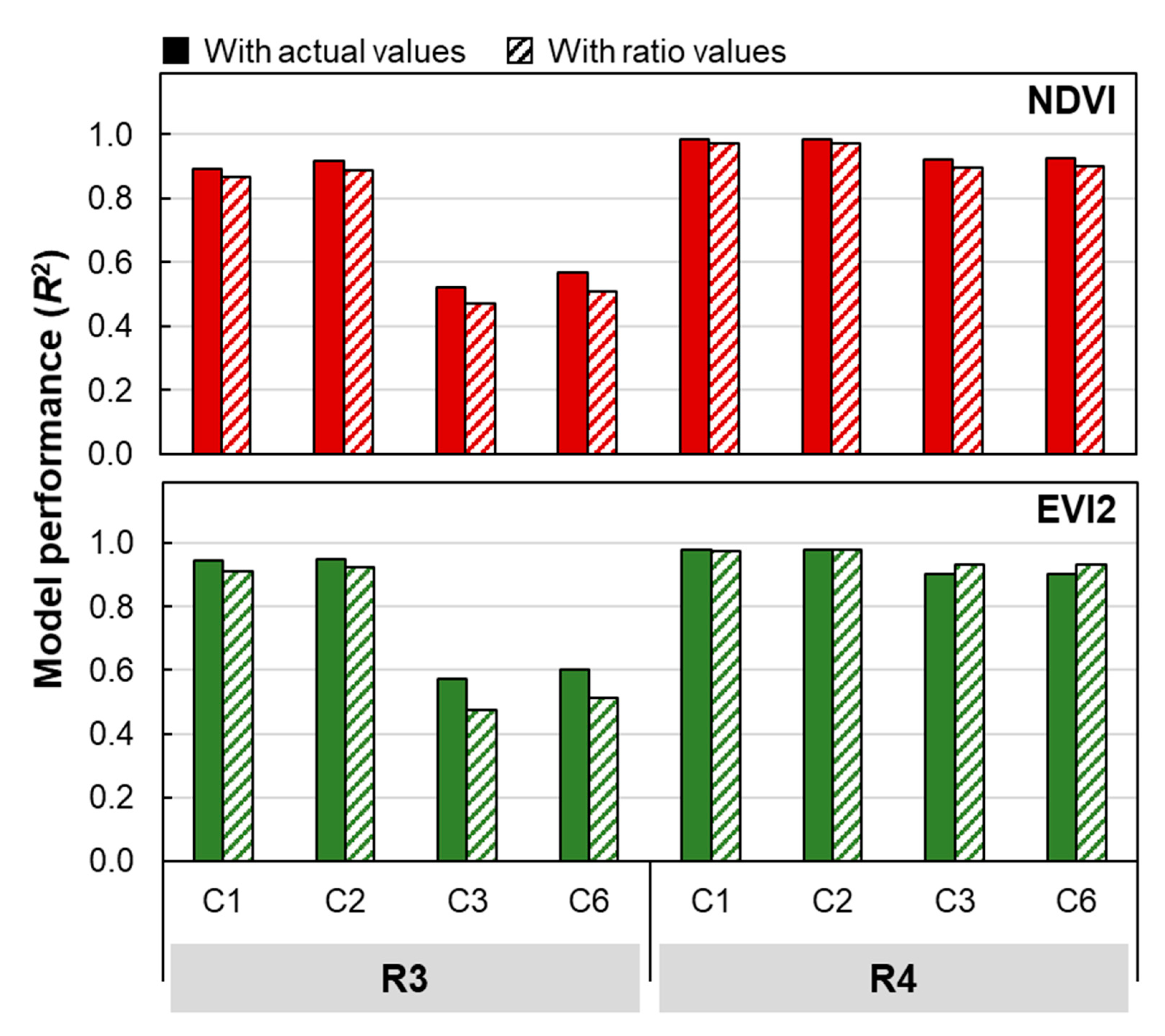
The use of yield and NDVI ratios (relative to the N-rich control) showed comparable accuracy to models derived directly from yield and NDVI (Figure 8). With ratio models, NDVI values were normalized against NDVI of the N-rich strip, thus adding variability. For relative yield estimations, the images captured at R3 and R4 with sidedress combinations C1 (zero-N + N-rich) and C2 (zero-N + N at V4) produced reliable estimates (R2 > 0.87). The models performed well (R2 > 0.92) with images captured at R4 with all selected sidedress combinations (C1, C2, C3, and C6). Sensing at R3 produced a lower R2 when plots that were sidedressed at V6 were included. These results show more accurate predictions than [41], which demonstrated a linear relationship between relative NDVI and relative yield in Nebraska when sensed at V11 and V15, achieving an R2 of 0.76.
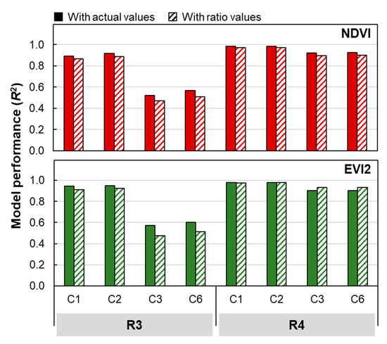
Figure 8.
Comparison of corn yield estimation model performance with actual and ratio values of selected vegetation indices and selected sidedress treatment combinations from the UAS imagery obtained at R3 and R4. Note: C1 indicates zero-N + N-rich (all N applied at planting), C2 indicates zero-N + sidedressing at V4, C3 indicates zero-N + N-rich + sidedressing at V6, and C6 indicates zero-N + N-rich + V4 + V6.
Consistent with our findings for yield models from actual yield values, the model performance of ratio models indicated a slight reduction in R2 when zero-N was not included in the model, although the reduction in R2 was minimal (Figure 9). The results suggest that it is possible for the combination of N-rich + V6 without zero-N to produce reliable yield estimates when images are captured at R4 (R2 values ranged between 0.86 and 0.97 for the NDVI ratio). The reduction in accuracy when zero-N was excluded in the ratio model for EVI2 provides further evidence that NDVI is the better VI for yield estimation.

Figure 9.
Model performance of selected vegetation indices ratio and selected sidedress treatment combinations, with and without zero-N treatments, at R3 and R4 growth stages.
3.7. Effect of Sampling Area on Yield Estimation Models
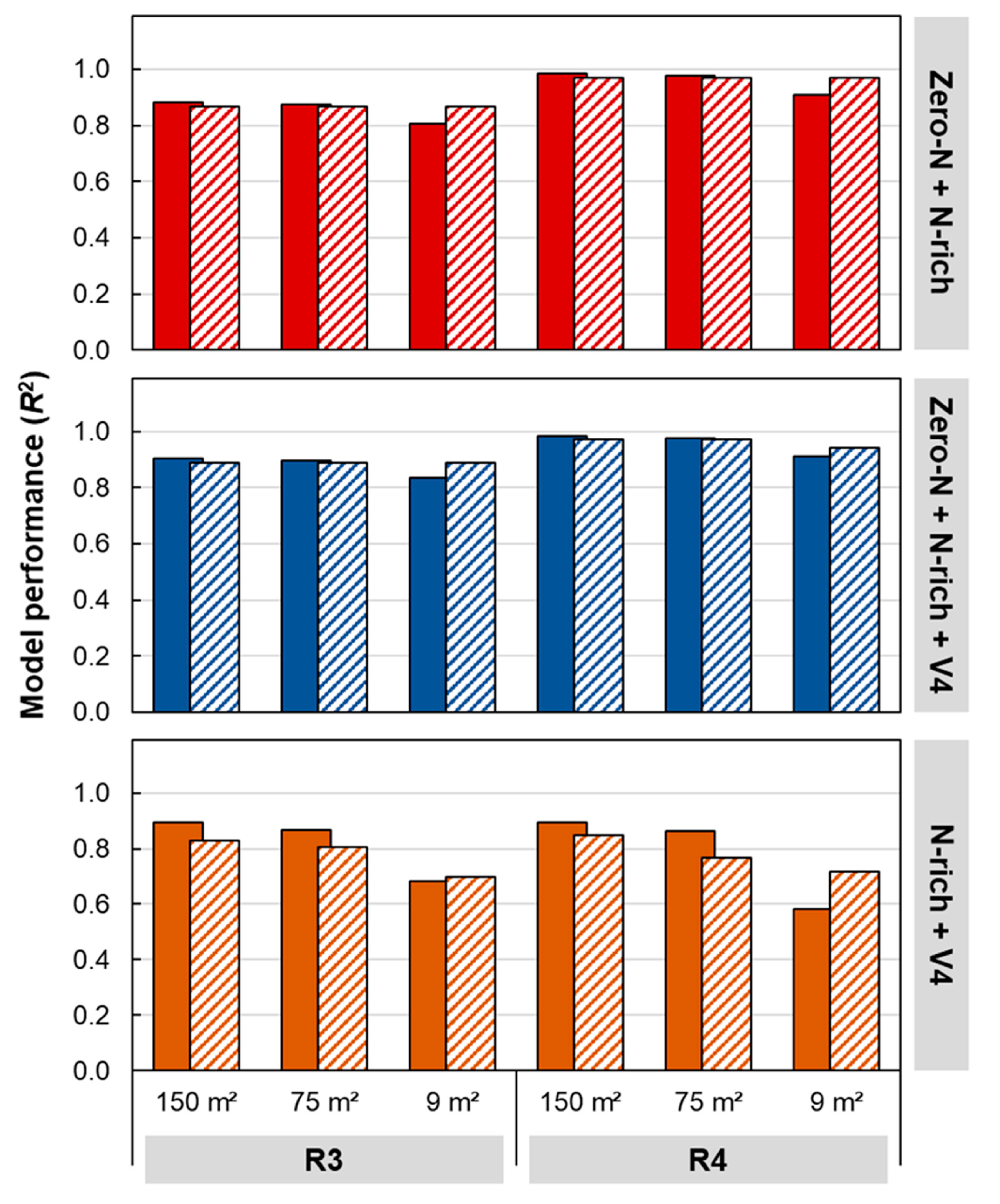
Model R2 decreased with the decrease in sample area (increase in number of subplots) but yield estimation models with actual values versus ratios remained comparable across sampling area sizes (Figure 10). These results are consistent with a previous study by [17], which reported that reducing the sampling area (three areas tested) increased yield estimation errors. It is likely that with a smaller sampling area, more yield and vegetation index variabilities are introduced, which in turn reduces model performance. Another study [3] used a rectangular polygon of fixed dimension (the product of harvester width and distance over each yield monitor data point) to predict yield from soil properties, achieving R2 = 0.53 using a random forest model. Although the random forest model theoretically accounts for the existence of nonlinear relationships, the lower R2 is likely due to the increased number of subplots with the use of polygons [3]. The smallest sampling area evaluated in this New York study was smaller than the area used by [3]. Yet, the current study produced a higher accuracy, which can be attributed to the placement of the control N treatments. The reduction in model performance with smaller sampling area size may not be significant in our study, but it requires further study across multiple fields and years to determine an optimum sampling area for the development of yield estimation models.
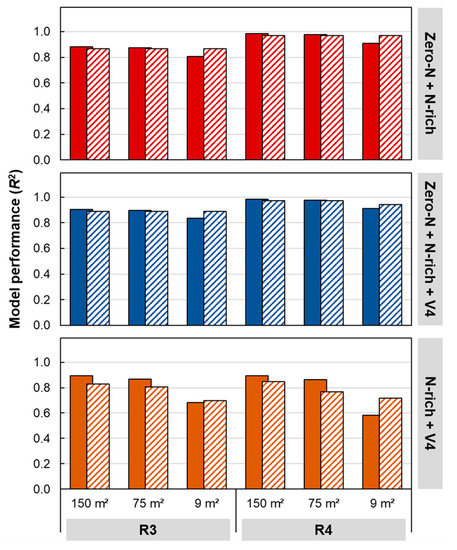
Figure 10.
Corn yield estimation model performance at different sampling areas using actual yield and NDVI (solid bars) and yield ratio models (hashed bars) of selected sidedress treatment combinations.
3.8. Selected Yield Estimation Models and the Estimated Yield Maps
The validation results using NDVI obtained at R4 as the independent variable, and using three sidedress combinations at three plot sizes, showed that the sampling area should be restricted to whole or half strips (at least 75 m2), especially when the zero-N treatment is not included (Table 1). Similar to previous studies [11,17,25], the results here suggest that an N-rich strip allows for calibration of the yield and reflectance signals, which results in more reliable yield estimates.

Table 1.
Performance of the fitted exponential models with selected sidedress combinations at three sampling areas from the flight at R4, using leave-one-out cross-validation.
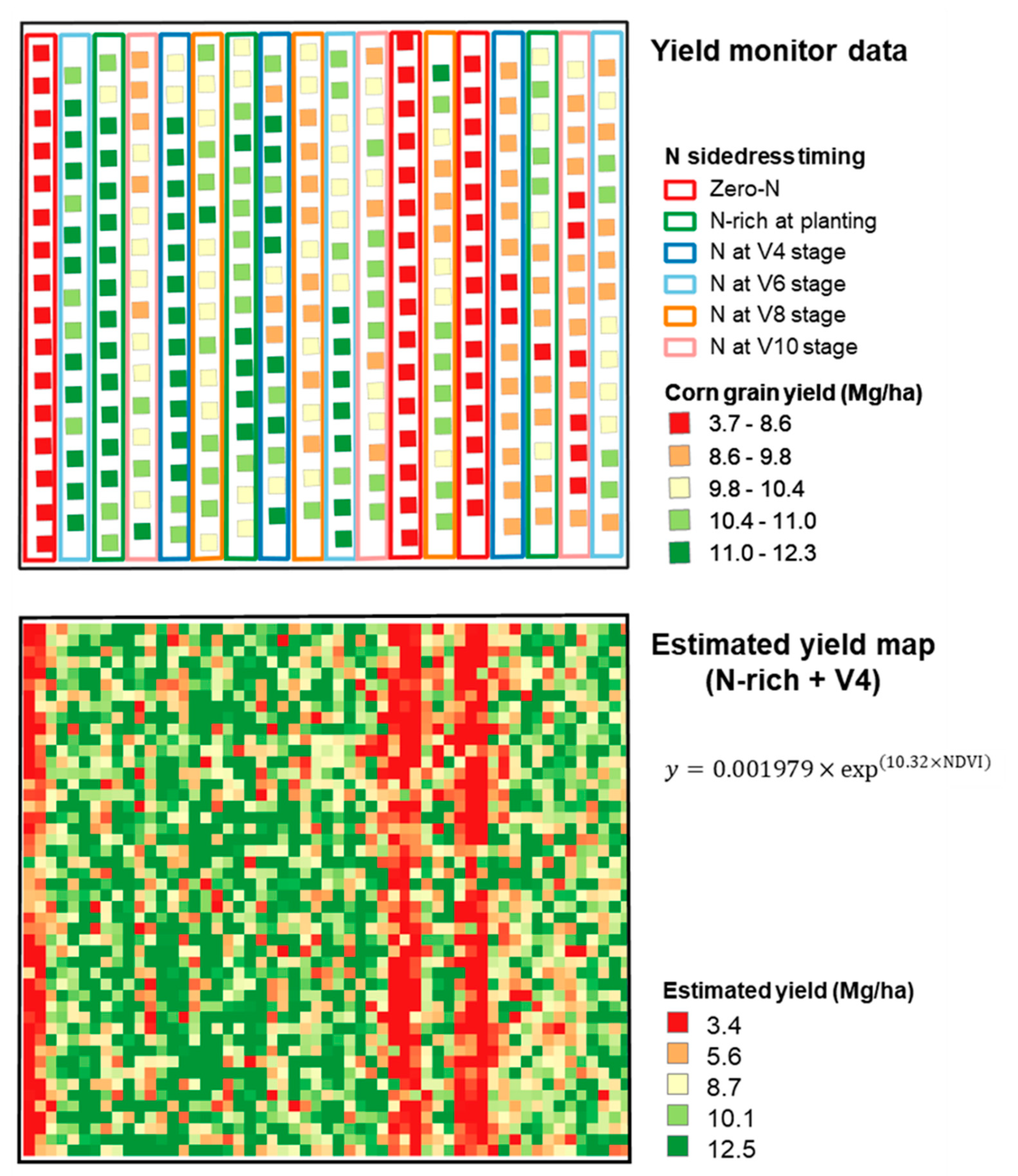
A yield map, derived using N-rich + V4, highlighted the zero-N treatments (Figure 11), thus indicating that these low-yielding areas were easily identified in the estimated yield maps generated from UAS imagery. Ranges in actual yield and estimated yield were almost identical, ranging from 3.7 to 12.3 Mg ha−1 (actual) versus from 3.4 to 12.5 Mg ha−1 (based on NDVI).
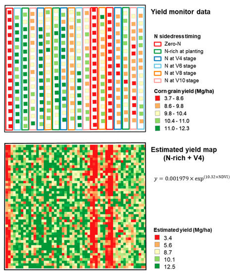
Figure 11.
The actual corn yield map (yield monitor system) compared with yield maps estimated based on NDVI from N-rich and V4 plots, using a raster calculator at 1 m/pixel spatial resolution.
4. Conclusions
This study had as its main objectives to compare various vegetation indices for their ability to estimate yield (R4 growth stage), to assess the effect of sidedress application timing on yield estimation (again at the R4 growth stage), to evaluate the impact of the growth stage/timing on VI-based corn yield prediction models, and to determine whether the zero-N strip (control) is essential for deriving accurate yield estimation models, while we also evaluated the effect of sampling area (plot size) on model accuracy. Among the six vegetation indices tested, the NDVI and EVI2 were most suitable for estimating corn grain yield. The inclusion of imagery from plots where sidedressing was performed after V6 resulted in less reliable predictions, while sensing before R1 also resulted in lower model performance. We determined that, for reasonable yield estimation (R2 > 0.80), sensing should be performed at stages R1−R4 using plots where sidedressing took place at or before V4 during stable illumination conditions. The use of yield ratios, for expansion beyond individual fields, resulted in reliable models (R2 > 0.87) to estimate relative yield, with only slightly lower R2 than when direct yield and NDVI data were used. Eliminating zero-N treatments as a reference resulted in a slightly lower R2 as well. Model R2 was impacted by sampling area, with higher R2 observed with a large sampling area compared to a smaller area (this was attributed to data averaging, or reduced variability, due to averaging across multiple points). However, the model performances were comparable between yield models with actual (NDVI vs. yield) and ratio values (NDVI ratio vs. yield ratio) across sampling areas (9, 75 m2, and 150 m2). Finally, we concluded that the most accurate corn grain yield estimations can be obtained using plots with N-rich + V4, with or without zero-N, sensed via NDVI at R3 or R4.
These results bode well for eventual implementation by growers or service providers, as their implementation requires readily accessible, relatively affordable four-band imagery that contains a NIR channel. Such systems have become ubiquitous in the UAS realm, and the addition of a downwelling sensor that allows for real-time calibration has enabled seamless operation and reliable imagery for modeling purposes. The caveats are that practitioners should follow recommended guidelines in terms of when imagery is obtained during the growing season (as found in the present study) and that imagery ideally should be collected under stable illumination conditions. We recommend that future research focuses on the extension of our results to other regions and, critically, that model improvement under typical operational conditions, i.e., irrespective of weather conditions, be evaluated.
Author Contributions
Conceptualization, S.S., Q.M.K., J.C. and J.G.; methodology, S.S., Q.M.K. and J.G.; software, S.S.; validation, S.S. and Q.M.K.; formal analysis, S.S.; investigation, S.S.; resources, Q.M.K.; data curation, S.S., J.C., J.G. and J.v.A.; writing—original draft preparation, S.S. and Q.M.K.; writing—review and editing, Q.M.K., K.J.C., J.G. and J.v.A.; visualization, S.S.; supervision, Q.M.K., K.J.C., J.G. and J.v.A.; project administration, Q.M.K.; funding acquisition, Q.M.K. All authors have read and agreed to the published version of the manuscript.
Funding
This research was funded in part with Federal Formula Funds and through grants from the New York Farm Viability Institute (NYFVI) and New York State Department of Environmental Conservation (NYDEC). J.G. received support from the National Science Foundation under grant No. 1916208.
Acknowledgments
Authors would like to thank Paul Stachowski, farm supervisor, Musgrave Research Farm, Aurora, NY, for providing us with the yield monitor data and managing field activities; Greg Godwin, Research support specialist with the Nutrient Management Spear Program, Cornell University, Ithaca, NY, for collecting weekly UAS flights, and processing and cleaning the yield monitor data.
Conflicts of Interest
The authors declare no conflict of interest. The funders had no role in the design of the study; in the collection, analyses, or interpretation of data; in the writing of the manuscript, or in the decision to publish the results.
References
- Long, E.A.; Ketterings, Q.M. Factors of Yield Resilience under Changing Weather Evidenced by a 14-Year Record of Corn-Hay Yield in a 1000-Cow Dairy Farm. Agron. Sustain. Dev. 2016, 36, 16. [Google Scholar] [CrossRef] [Green Version]
- Kharel, T.P.; Maresma, A.; Czymmek, K.J.; Oware, E.K.; Ketterings, Q.M. Combining Spatial and Temporal Corn Silage Yield Variability for Management Zone Development. Agron. J. 2019, 111, 2703. [Google Scholar] [CrossRef]
- Khanal, S.; Fulton, J.; Klopfenstein, A.; Douridas, N.; Shearer, S. Integration of High Resolution Remotely Sensed Data and Machine Learning Techniques for Spatial Prediction of Soil Properties and Corn Yield. Comput. Electron. Agric. 2018, 153, 213–225. [Google Scholar] [CrossRef]
- Cisternas, I.; Velásquez, I.; Caro, A.; Rodríguez, A. Systematic Literature Review of Implementations of Precision Agriculture. Comput. Electron. Agric. 2020, 176, 105626. [Google Scholar] [CrossRef]
- Karthikeyan, L.; Chawla, I.; Mishra, A.K. A Review of Remote Sensing Applications in Agriculture for Food Security: Crop Growth and Yield, Irrigation, and Crop Losses. J. Hydrol. 2020, 586, 124905. [Google Scholar] [CrossRef]
- Neto, A.J.S.; Lopes, D.C.; Pinto, F.A.; Zolnier, S. Vis/NIR Spectroscopy and Chemometrics for Non-Destructive Estimation of Water and Chlorophyll Status in Sunflower Leaves. Biosyst. Eng. 2017, 155, 124–133. [Google Scholar] [CrossRef]
- Tucker, C.J. Red and Photographic Infrared Linear Combinations for Monitoring Vegetation. Remote Sens. Environ. 1979, 8, 127–150. [Google Scholar] [CrossRef] [Green Version]
- Maresma, A.; Chamberlain, L.; Tagarakis, A.; Kharel, T.; Godwin, G.; Czymmek, K.J.; Shields, E.; Ketterings, Q.M. Accuracy of NDVI-Derived Corn Yield Predictions Is Impacted by Time of Sensing. Comput. Electron. Agric. 2020, 169, 105236. [Google Scholar] [CrossRef]
- Raun, W.R.; Solie, J.B.; Johnson, G.V.; Stone, M.L.; Lukina, E.V.; Thomason, W.E.; Schepers, J.S. In-Season Prediction of Potential Grain Yield in Winter Wheat Using Canopy Reflectance. Agron. J. 2001, 93, 131–138. [Google Scholar] [CrossRef] [Green Version]
- Raun, W.R.; Solie, J.B.; Stone, M.L.; Zavodny, D.L.; Martin, K.L.; Freeman, K.W. Automated Calibration Stamp Technology for Improved In-season Nitrogen Fertilization. Agron. J. 2005, 97, 5. [Google Scholar]
- Tagarakis, A.C.; Ketterings, Q.M. Proximal Sensor-Based Algorithm for Variable Rate Nitrogen Application in Maize in Northeast U.S.A. Comput. Electron. Agric. 2018, 145, 373–378. [Google Scholar] [CrossRef]
- Tagarakis, A.C.; Ketterings, Q.M. In-Season Estimation of Corn Yield Potential Using Proximal Sensing. Agron. J. 2017, 109, 1323–1330. [Google Scholar] [CrossRef] [Green Version]
- Barzin, R.; Pathak, R.; Lotfi, H.; Varco, J.; Bora, G.C. Use of UAS Multispectral Imagery at Different Physiological Stages for Yield Prediction and Input Resource Optimization in Corn. Remote Sens. 2020, 12, 2392. [Google Scholar] [CrossRef]
- Gao, F.; Anderson, M.; Daughtry, C.; Johnson, D. Assessing the Variability of Corn and Soybean Yields in Central Iowa Using High Spatiotemporal Resolution Multi-Satellite Imagery. Remote Sens. 2018, 10, 1489. [Google Scholar] [CrossRef] [Green Version]
- Kayad, A.; Sozzi, M.; Gatto, S.; Marinello, F.; Pirotti, F. Monitoring Within-Field Variability of Corn Yield Using Sentinel-2 and Machine Learning Techniques. Remote Sens. 2019, 11, 2873. [Google Scholar] [CrossRef] [Green Version]
- Kross, A.; Znoj, E.; Callegari, D.; Kaur, G.; Sunohara, M.; Lapen, D.R.; McNairn, H. Using Artificial Neural Networks and Remotely Sensed Data to Evaluate the Relative Importance of Variables for Prediction of Within-Field Corn and Soybean Yields. Remote Sens. 2020, 12, 2230. [Google Scholar] [CrossRef]
- Zhang, M.; Zhou, J.; Sudduth, K.A.; Kitchen, N.R. Estimation of Maize Yield and Effects of Variable-Rate Nitrogen Application Using UAV-Based RGB Imagery. Biosyst. Eng. 2020, 189, 24–35. [Google Scholar] [CrossRef]
- Deines, J.M.; Patel, R.; Liang, S.-Z.; Dado, W.; Lobell, D.B. A Million Kernels of Truth: Insights into Scalable Satellite Maize Yield Mapping and Yield Gap Analysis from an Extensive Ground Dataset in the US Corn Belt. Remote Sens. Environ. 2021, 253, 112174. [Google Scholar] [CrossRef]
- Pantazi, X.E.; Moshou, D.; Alexandridis, T.; Whetton, R.L.; Mouazen, A.M. Wheat Yield Prediction Using Machine Learning and Advanced Sensing Techniques. Comput. Electron. Agric. 2016, 121, 57–65. [Google Scholar] [CrossRef]
- Yang, W.; Nigon, T.; Hao, Z.; Paiao, G.D.; Fernández, F.G.; Mulla, D.; Yang, C. Estimation of Corn Yield Based on Hyperspectral Imagery and Convolutional Neural Network. Comput. Electron. Agric. 2021, 184, 106092. [Google Scholar] [CrossRef]
- Maresma, Á.; Ariza, M.; Martínez, E.; Lloveras, J.; Martínez-Casasnovas, J. Analysis of Vegetation Indices to Determine Nitrogen Application and Yield Prediction in Maize (Zea mays L.) from a Standard UAV Service. Remote Sens. 2016, 8, 973. [Google Scholar] [CrossRef] [Green Version]
- Peralta, N.; Assefa, Y.; Du, J.; Barden, C.; Ciampitti, I. Mid-Season High-Resolution Satellite Imagery for Forecasting Site-Specific Corn Yield. Remote Sens. 2016, 8, 848. [Google Scholar] [CrossRef] [Green Version]
- Gopalapillai, S.; Tian, L. In-Field Variability Detection and Spatial Yield Modeling for Corn Using Digital Aerial Imaging. Trans. ASAE 1999, 42, 1911. [Google Scholar] [CrossRef]
- Sripada, R.P.; Schmidt, J.P.; Dellinger, A.E.; Beegle, D.B. Evaluating Multiple Indices from a Canopy Reflectance Sensor to Estimate Corn N Requirements. Agron. J. 2008, 100, 1553–1561. [Google Scholar] [CrossRef]
- Holland, K.H.; Schepers, J.S. Use of a Virtual-Reference Concept to Interpret Active Crop Canopy Sensor Data. Precis. Agric. 2013, 14, 71–85. [Google Scholar] [CrossRef]
- Northeast Regional Climate Center CLIMOD2. Available online: http://climod2.nrcc.cornell.edu/ (accessed on 24 July 2020).
- Kharel, T.P.; Swink, S.N.; Youngerman, C.; Maresma, A.; Czymmek, K.J.; Ketterings, Q.M.; Kyveryga, P.; Lory, J.; Musket, T.A.; Hubbard, V. Processing/Cleaning Corn Silage and Grain Yield Monitor Data for Standardized Yield Maps across Farms, Fields, and Years; Nutrient Management Spear Program, Department of Animal Science, Cornell University: Ithaca, NY, USA, 2018. [Google Scholar]
- Kharel, T.P.; Swink, S.N.; Maresma, A.; Youngerman, C.; Kharel, D.; Czymmek, K.J.; Ketterings, Q.M. Yield Monitor Data Cleaning Is Essential for Accurate Corn Grain and Silage Yield Determination. Agron. J. 2019, 111, 509–516. [Google Scholar] [CrossRef]
- R Core Team. R: A Language and Environment for Statistical Computing; R Foundation for Statistical Computing: Vienna, Austria, 2019; Available online: https://www.R-project.org/ (accessed on 30 September 2021).
- Bates, D.; Mächler, M.; Bolker, B.; Walker, S. Fitting Linear Mixed-Effects Models Using Lme4. arXiv 2014, arXiv:1406.5823. Available online: https://arxiv.org/abs/1406.5823 (accessed on 30 September 2021).
- Lenth, R.V. Least-Squares Means: The R Package Lsmeans. J. Stat. Softw. 2016, 69, 1–33. [Google Scholar] [CrossRef] [Green Version]
- Purucker, T.S.; Steinke, K. Comparing Nitrogen Timing and Sidedressing Placement Strategies on Corn Growth and Yield in Michigan. Crop Forage Turfgrass Manag. 2020, 6, e20033. [Google Scholar] [CrossRef]
- Walsh, O.; Raun, W.; Klatt, A.; Solie, J. Effect of Delayed Nitrogen Fertilization on Maize (Zea mays L.) Grain Yields and Nitrogen Use Efficiency. J. Plant Nutr. 2012, 35, 538–555. [Google Scholar] [CrossRef] [Green Version]
- Rutan, J.; Steinke, K. Pre-Plant and In-Season Nitrogen Combinations for the Northern Corn Belt. Agron. J. 2018, 110, 2059–2069. [Google Scholar] [CrossRef] [Green Version]
- Scharf, P.C.; Wiebold, W.J.; Lory, J.A. Corn Yield Response to Nitrogen Fertilizer Timing and Deficiency Level. Agron. J. 2002, 94, 435–441. [Google Scholar] [CrossRef]
- Hunt, E.R., Jr.; Doraiswamy, P.C.; McMurtrey, J.E.; Daughtry, C.S.; Perry, E.M.; Akhmedov, B. A Visible Band Index for Remote Sensing Leaf Chlorophyll Content at the Canopy Scale. Int. J. Appl. Earth Obs. Geoinf. 2013, 21, 103–112. [Google Scholar] [CrossRef] [Green Version]
- Jiang, Z.; Huete, A.R.; Didan, K.; Miura, T. Development of a Two-Band Enhanced Vegetation Index without a Blue Band. Remote Sens. Environ. 2008, 112, 3833–3845. [Google Scholar] [CrossRef]
- Liu, J.; Huffman, T.; Qian, B.; Shang, J.; Li, Q.; Dong, T.; Davidson, A.; Jing, Q. Crop Yield Estimation in the Canadian Prairies Using Terra/MODIS-Derived Crop Metrics. IEEE J. Sel. Top. Appl. Earth Obs. Remote Sens. 2020, 13, 2685–2697. [Google Scholar] [CrossRef]
- Bolton, D.K.; Friedl, M.A. Forecasting Crop Yield Using Remotely Sensed Vegetation Indices and Crop Phenology Metrics. Agric. For. Meteorol. 2013, 173, 74–84. [Google Scholar] [CrossRef]
- Joshi, V.R.; Thorp, K.R.; Coulter, J.A.; Johnson, G.A.; Porter, P.M.; Strock, J.S.; Garcia y Garcia, A. Improving Site-Specific Maize Yield Estimation by Integrating Satellite Multispectral Data into a Crop Model. Agronomy 2019, 9, 719. [Google Scholar] [CrossRef] [Green Version]
- Solari, F.; Shanahan, J.; Ferguson, R.; Schepers, J.; Gitelson, A. Active Sensor Reflectance Measurements of Corn Nitrogen Status and Yield Potential. Agron. J. 2008, 100, 571–579. [Google Scholar] [CrossRef] [Green Version]
Publisher’s Note: MDPI stays neutral with regard to jurisdictional claims in published maps and institutional affiliations. |
© 2021 by the authors. Licensee MDPI, Basel, Switzerland. This article is an open access article distributed under the terms and conditions of the Creative Commons Attribution (CC BY) license (https://creativecommons.org/licenses/by/4.0/).

