A Fast Hyperspectral Anomaly Detection Algorithm Based on Greedy Bilateral Smoothing and Extended Multi-Attribute Profile

Abstract

To address the difficulty of separating background materials from similar materials associated with the use of “single-spectral information” for hyperspectral anomaly detection, a fast hyperspectral anomaly detection algorithm based on what we term the “greedy bilateral smoothing and extended multi-attribute profile” (GBSAED) method is proposed to improve detection precision and operation efficiency. This method utilizes “greedy bilateral smoothing” to decompose the low-rank part of a hyperspectral image (HSI) dataset and calculate spectral anomalies. This process improves the operational efficiency. Then, the extended multi-attribute profile is used to extract spatial anomalies and restrict the shape of anomalies. Finally, the two components are combined to limit false alarms and obtain appropriate detection results. This new method considers both spectral and spatial information with an improved structure that ensures operational efficiency. Using five real HSI datasets, this study demonstrates that the GBSAED method is more robust than eight representative algorithms under diverse application scenarios and greatly improves detection precision and operational efficiency.

1. Introduction

A hyperspectral image (HSI) is an image data product containing rich spatial and spectral information. An HSI includes hundreds of nearly continuous spectral bands [1,2,3]. Compared to traditional optical and multispectral images, HSIs convey more features, significantly improving the ability to detect subtle differences in the characteristics of different materials [4]. Therefore, it offers unique advantages for classification and target detection [5,6,7,8,9].

Target detection is essentially a binary classification problem that aims to extract specific pixels from images with various backgrounds. Target detection is a major application of HSI processing and is crucial in situations such as battle reconnaissance, hostage rescue, and ecological supervision [10,11]. However, those practical applications lack prior information and thus require unsupervised anomaly target detection [12], which has become a focus of recent research [6,13,14,15,16,17].

In the past few decades, a large number of anomaly detection algorithms have been proposed and improved. These algorithms are of two main types, namely statistical modeling algorithms and representation-based algorithms [18]. These statistical modeling methods are often related to the Gaussian distribution. For hyperspectral anomaly detection, the benchmark is the typical Reed-Xiaoli (RX) algorithm [19]. RX assumes that the background model conforms to a multidimensional Gaussian distribution and obtains detection results from the Mahalanobis distance between the spectral mean of selected pixels and the background pixels. This process impairs the performance of the statistics-based detector due to contamination with abnormal data in the background statistics, improper modeling of the Gaussian distribution, and the usage of lower-order information. Many improved RX algorithms have been proposed to address these problems [20,21,22,23,24,25,26]. Representatives of these algorithms include subspace RX (SSRX) [20], regularized RX [21], kernel RX (KRX) [22], cluster kernel RX (CKRX) [23], cluster-based anomaly detection (CBAD) [24], weighted RX [25], and blocked adaptive computationally efficient outlier nominators (BACON) [26]. However, those algorithms do not solve the central problem, as they employ assumptions for the data. Therefore, their results are easily influenced by complex or contaminated backgrounds.

Recently, representation-based algorithms have been widely applied to hyperspectral remote sensing [27,28,29,30,31,32,33], such as collaborative representation-based detector (CRD) [27], background joint sparse representation detector (BJSRD) [28], low-rank and sparse representation-based detector (LRASR) [29] and low-rank and sparse matrix decomposition-based anomaly detection method (LRaSMD) [33]. These methods require no statistical assumptions. During processing, background pixels can be expressed as linear combinations of background dictionaries, while abnormal pixels cannot. Residual errors are defined by the degree of anomaly of the pixel, with large residual error reflecting a greater likelihood of anomaly.

Starting with the inherent attributes of the HSI, the low-rank and sparse matrix decomposition-based anomaly detection method (LRaSMD) assumes low-rankness of the spectral vector of background pixels, represented by base vector linear combinations, as well as sparseness of the anomaly target, which occurs with low probability in small quantities [33]. Therefore, the LRaSMD method decomposes the original HSI into low-rank, sparse, and noise matrices. Some LRaSMD methods show relatively good performance in hyperspectral anomaly detection, including Euclidean distance-based LRaSMD (EDLRaSMD) [34], two-norm-based LRaSMD [35], the LRaSMD-based Mahalanobis distance method for hyperspectral anomaly detection (LSMAD) [36] and the parts representation-based LRaSMD (PRLRaSAD) [4].

LRaSMD considers the low-rankness of the background and sparsity of anomalies to decompose low-rank and sparse components. This method is effective for addressing the problem of anomaly detection and avoids a situation in which a larger sample number in the neighboring window algorithm may increase the complexity and difficulty of the operation process [4]. However, some background components may be classified as sparse parts due to noise in the image caused by complex ground object types, the presence of background objects with sparseness and few pixels, environmental changes, or sensor problems [37]. In addition, such detectors generally use the pixel’s spectral features but ignore their spatial distribution characteristics [38], influencing detection performance. Moreover, most methods based on LRaSMD are time-consuming.

The present study introduces a fast hyperspectral anomaly detection algorithm based on what we term the “greedy bilateral smoothing and extended multi-attribute profile” (GBSAED) method. In this method, the extended multi-attribute profile is effectively applied for modeling of spatial information. From spatial and spectral perspectives, the LRaSMD model decomposes the background and applies the extended morphological attribute profile (EMAP) to obtain data representing the spatial feature. Then, the Mahalanobis distance is employed to construct spectral anomaly components and spatial anomaly components. Finally, information from each process is integrated to obtain the final detection result. In this study, the GBSAED method showed good performance when applied to five real hyperspectral datasets.

The structure of this paper is organized as follows. The second section introduces the basic concepts of EMAP and LRaSMD method. The third section presents the proposed algorithm. The fourth section describes and discusses the experiments conducted using five datasets. Finally, the fifth section summarizes the full study.

2. Related Work

2.1. Low-Rank and Sparse Matrix Decomposition

In hyperspectral data, adjacent pixels have similar spectral vectors because they have similar qualities [39]. Due to the strong correlations among bands, the spectral vectors of smooth and continuous background pixels in HSI can be approximately represented as linear combinations of several base vectors. Thus, the background of HSI is characterized by low rankness in low-dimensionality subspace. In contrast to background pixels, anomalous pixels account for a small proportion of the image. Assuming that these pixels are distributed randomly, anomalous pixels are characterized by sparsity. The LRaSMD method treats the matrix as the sum of low-rank, sparse, and noise matrices. This process can describe the low-rankness and sparsity of HSI background and anomalous features. This method does not aim to establish a single model for each feature, but instead considers the two feature types simultaneously to extract useful information from the noise and acquire additional background components from restored data. The LRaSMD algorithm is represented by Equation (1) [40].

$$X=B+A+N$$

(1)

where $X\in {ℝ}^{n\times b}$. (n and b represent pixel number and band number, respectively). B is the low-rank matrix representing spectral information for the image background. A is the sparse matrix representing spectral information for the anomaly target. N is the noise matrix. Noise in the image is assumed to be a Gaussian random variable.

$$\min \parallel X-B-A{\parallel }_F^2,\mathrm{rank}\left(B\right)\le rcard\left(A\right)\le kn$$

(2)

The algorithm establishes a minimized decomposition error function by controlling model complexity through limiting the rank of the low-rank matrix B and sparsity of the sparse matrix A. Equation (1) can then be rewritten as Equation (2).

Where r and k denote the rank of the low-rank matrix and sparsity of the sparse matrix. This equation can effectively express background information by controlling the maximum value of r. k expresses the occurrence probability of anomalous pixels in the image. As the number of iterations increases, decomposition error shows a monotonic decreasing trend. Therefore, Equation (2) can be transformed into two sub-problems; their functions are shown as Equation (3).

$$\begin{array}{c}{B}_t=\underset{\mathrm{rank}\left(B\right)⩽r}{\mathrm{argmin}}\parallel X-B-A_{t-1}\parallel {}_F^2\\ S_t=\underset{\mathrm{card}\left(A\right)⩽kn}{\mathrm{argmin}}\parallel X-B_{t-1}-A{\parallel }_F^2\end{array}$$

(3)

where B_t and S_t represent the optimal solution at the tth iteration. When decomposition errors uniformly converge to a local minimum, iteration stops and the low-rank matrix B, sparse matrix A, and noise matrix N are constructed.

2.2. Extended Morphological Attribute Profile

Attribute profiles (APs) originate from the morphological profile [41]. APs are based on attribute filters that operate using an image’s connected components (CC). Through two basic operators, thinning and thickening, filtration produces a series of image sequences. This process compares each CC’s attributes and threshold value, $\beta$, and then estimates whether this region satisfies the set standard. If not, the value is set to the nearest radiation value in the adjacent domain, merging that region into the adjacent CC. This domain can be merged into an adjacent domain with a lower or higher grayness level, resulting in thinning and thickening, respectively. The function underlying this process is given by Equation (4).

$$AP\left(f\right)=\left\{{\varphi }_n(f),{\varphi }_{n-1}(f),\dots ,{\varphi }_1(f),f,{\gamma }_1(f),{\gamma }_2(f),\dots ,{\gamma }_n(f)\right\}\mathrm{r}$$

(4)

where ${\gamma }_i$ and ${\varphi }_i,\left(i=1,2,\dots ,n\right)$ represent thinning and thickening, respectively.

However, APs are not easily expanded into multiple-value data (e.g., HSI data) because the sequence of data elements is not contained within the native definition [42]. An extended AP (EAP) method for spatial feature extraction of HSIs is proposed to solve this problem. This technique connects APs with the same attributes for a number of principal components extracted from the original image. Then, one EAP is calculated using Equation (5).

$$EAP=\left\{AP\left(f_{PC}\right),AP\left(f_{P{C}_2}\right),\dots ,AP\left(f_{P{C}_p}\right)\right\}$$

(5)

EMAP method was proposed in [43]. Compared to EAP, EMAP method considers numerous attributes as a whole. This allows for further exploration of spatial features in HSI modeling.

3. Proposed Method

3.1. GBSAED Method Flowchart

Figure 1 is a flowchart of the GBSAED method. It includes three steps: fast extraction of low-rank information based on “greedy bilateral smoothing”; extraction of spatial information based on EMAP method; and complementation of spectral and spatial anomalies based on Mahalanobis distance. The third step uses spatial anomalies to restrict spectral anomalies, which reduces the false alarm rate, and then determines the result.

3.2. Fast Extraction of Abnormal Spectral Features Using Greedy Bilateral Smoothing

According to the description of the LRaSMD method provided in Section II, the model rebuilds HSI data into $X=B+A+N$ ($X\in {ℝ}^{n\times b}$). For the additive noise matrix N, the greedy bilateral smoothing method proposed by Zhou and Tao [44] is employed to reduce the time cost of single-value decomposition at each iteration in the traditional LRaSMD model. We replaced the low-rank matrix B with the bilateral factor B = MN and regularized the norm ℓ1 of sparse matrix A. This process is represented by Equation (6).

$$\begin{array}{c}\underset{M,N,A}{\min }\parallel X-MN-A{\parallel }_F^2+\lambda \parallel A{\parallel }_1\\ \mathrm{s}.\mathrm{t}.\mathrm{rank}\left(M\right)=\mathrm{rank}\left(N\right)\le r\end{array}$$

(6)

where $\lambda$ is a regularization parameter. To solve Equation (6), this method introduces a soft threshold ${\mathcal{S}}_{\lambda }X=\mathrm{sgn}\left(X\right)\cdot \max \left(\left|X\right|-\lambda ,0\right)$ during regularization of ℓ1 and updating of A. ${\mathcal{S}}_{\lambda }$ is the soft threshold operator for $\lambda$. Alternate optimization of M, N, and A in Equation (6) leads to Equation (7).

$$M_k=\left(X-A_{k-1}\right)N_{k-1}^T{\left(N_{k-1}{N}_{k-1}^T\right)}^{†}{N}_k={\left(M_k^T{M}_k\right)}^{†}{M}_k^T\left(X-A_{k-1}\right)A_k={\mathcal{S}}_{\lambda }\left(X-M_k{N}_k\right)$$

(7)

where k denotes the number of iterations. ${(\cdot )}^{†}$ is the Moore-Penrose pseudo-inverse operation. Because MN and A codetermine the value of Equation (6) rather than M or N individually, a pair of (M, N) can be found with the same product as (M_k, N_k) in Equation (7), leading to faster computation. Thus, Equation (7) can be rewritten as Equation (8).

$$M_k{N}_k=M_k{\left(M_k^T{M}_k\right)}^{†}{M}_k^T\left(X-A_{k-1}\right)={\mathcal{P}}_{M_k}\left(X-A_{k-1}\right)$$

(8)

where $\mathcal{P}$ is an orthogonal projection operator. According to Equation (7), the column space of $M_k$ can be represented on a random orthonormal basis using $\left(X-A_{k-1}\right)N_{k-1}^T$ columns. Based on $\left(X-A_{k-1}\right)N_{k-1}^T=QR$, the fast QR decomposition method, $M_k$ is transformed into Q, and $M_k{N}_k$ can be computed as $M_k{N}_k={\mathcal{P}}_Q\left(X-A_{k-1}\right)=Q{Q}^T\left(X-A_{k-1}\right)$. Then, a fast upgrading process was applied, as described in Equation (9).

$$M_k=Q{N}_k=Q^T\left(X-A_{k-1}\right)A_k={\mathcal{S}}_{\lambda }\left(X-M_k{N}_k\right)$$

(9)

In the GreBsmo method, Equation (9) iterates k times or until the object converges. Then, it adds $∆r$ rows to matrix N, reducing the object’s value. To determine the fastest decreasing trend, it greedily uses the added $∆r$ rows as the singular vector of the top $∆r$ of the partial derivative. Then, the rank of matrix N is added to $r_1=r_0+∆r$. This function is shown as Equation (10).

$$\frac{\partial \parallel X-MN-A{\parallel }_F^2}{\partial N}=X-MN-A$$

(10)

Upon reaching the set fault tolerance, rank r stops increasing.

Decomposed sparse components are generally considered to contain rich anomaly information. However, sparse components are susceptible to sparse parameters. The false alarm rate will be high if the small number of targets is not fully considered. Meanwhile, the background inhibitory effect is poor if important background component information is ignored in the low-rank component. Division into background and anomaly components can weaken the interference effect of anomalies on background statistics, so the decomposed low-rank component $F_{spec}=MN$ should be treated as an initial spectral anomaly feature.

3.3. Extracting Abnormal Spatial Features Based on the Extended Multi-Attribute Profile

Based on m, the number of principal components in the original HSI, an EAP is established. Then, the EAP is calculated as four EMAP features with four different attributes: area, the diagonal of the target outline, inertia moment, and regional homogeneity. Some out-of-rule false alarms can be filtered out due to the spatial information restraint. Figure 2 shows a random area with four EMAP maps. We employed the first three principal components of HSI data to generate 36 spatial features based on their attributes. These features were designated as $F_{spa}$.

3.4. Proposed GBSAED Algorithm

Anomaly detection based on spectral or spatial features often acquires similar anomaly targets, but different false alarms arise due to various types of attribute information. With spectrum-based anomaly detection methods, some background pixels have a larger initial detection value similar to anomalies because they account for a small number of pixels. However, the spatial features of such pixels are rarely similar in terms of other properties, such as area. Figure 3 shows an example with various false alarms in the initial results for spectral and spatial anomaly detection. Parts A–C in Figure 3 represent three background areas in San Diego that exhibit sparsity. Therefore, the algorithm considered similar anomaly targets and employed a strategy of mutual inhibition of the two backgrounds. This process reduced the false alarm rate.

The initial spatial anomaly feature detection is conducted based on Mahalanobis distance, as shown in Equation (11).

$$X_{spa}\left(x_i\right)={\left(x_i-\mu \right)}^T{\mathsf{\Gamma }}^{-1}\left(x_i-\mu \right)$$

(11)

where $x_i={\left[x_1,x_2,\dots ,x_b\right]}^T$ denotes the spatial feature vector of each pixel, and $\mu ={\left({\mu }_1,{\mu }_2,\dots ,{\mu }_b\right)}^T$ and $\mathsf{\Gamma }$ are the mean value and covariance matrix, respectively, of the input background data.

$${\mu }_b=\frac{1}{n}{{\displaystyle \sum }}_{i=1}^n{x}_i$$

(12)

$${\mathsf{\Gamma }}_b=\frac{1}{n}{\displaystyle \sum }_{i=1}^n\left(x_i-{\mu }_b\right){\left(x_i-{\mu }_b\right)}^T$$

(13)

The initial detection value $X_{spec}$ of the spectral anomaly feature is obtained similarly. Due to a rank defect in matrix inversion of the covariance matrix based on the low-rank background matrix, a large feature value is selected and the corresponding feature vector employs base vectors to approximate background components [36]. In this process, the number of feature values is equal to the rank value. The matrix inversion function is presented as Equation (14).

$${\mathsf{\Gamma }}_b^{-1}=V{A}^{-1}{V}^T={\displaystyle \sum }_{j=1}^r{\lambda }_j^{-1}{V}_j{V}_j^T$$

(14)

where $V=\left[V_1,V_2,\dots ,V_r\right]$ represents the vector matrix of the characteristic value, $A=\mathrm{diag}\left(\begin{array}{cccc}{\lambda }_1& {\lambda }_2& \cdots & {\lambda }_r\end{array}\right)$ is the characteristic value matrix, and ${\lambda }_1\ge {\lambda }_2\ge \cdots \ge {\lambda }_B$.

The values at the positions corresponding to $F_{spec}$ and $F_{spa}$ are multiplied to suppress false alarms that differ from each other. The detector output is calculated using Equation (15).

$$D_{GBAED}=dot\left(F_{spec},F_{spa}\right)$$

(15)

Finally, the detailed procedure of the GBSAED algorithm is shown in Algorithm 1.

Algorithm 1. GBSAED framework for hyperspectral anomaly detection

Input: Hyperspectral image; rank $r$ rank step $∆r$; power $k$; soft thresholding $\lambda$; tolerance $\tau$;

Output: A two-dimensional detection result. 1: Initialize $N\in {ℝ}^{r_0\times n}$ and A 2: while residual error ≤ $r$ do 3:      for k = 1 to K 4:              sequentially compute (9) 5:      end for 6:      Calculate the top ∆r right singular vectors v of $\partial f/\partial M$ in (10) 7:      Set $V:=\left[V;v\right]$ 8: end 9: Extract the first three principal components of the original HSI 10: Calculate and obtain a set of EMAP features and extract the first four principal components; 11: Calculate preliminary detection values via (11) 12: Calculate the detection result via (15)

4. Experimental Results and Analysis

4.1. Experiment Setup

In this section, five real HSI datasets with differing features are used to validate the effectiveness of the proposed GBSAED algorithm. Then, the proposed algorithm is compared to the eight most advanced algorithms, namely the RX, LRX, KRX, SSRX, CRD, GTVLRR, LSMAD, and PRLRaSAD algorithms. Finally, the effects of parameters with different values in each dataset on the detection results are discussed. The experimental platform is a computer containing an Intel Core i9-10900K CPU at 3.70 GHz with 64 GB RAM. All procedures were conducted in MATLAB R2018a.

4.2. Hyperspectral Datasets

(1) Texas Coast Image: an Airport-Beach-Urban (ABU) dataset of the Texas coast in the United States obtained by the airborne visible/infrared imaging spectrometer (AVIRIS) [45]. The image size is 100 × 100 pixels, with 207 spectral bands ranging from 450 to 1350 nm. Its spatial resolution is 17.2 m. The anomaly object of this image is a building, and the background object is vegetation. The dataset has serious stripe noise in the 144–153 and 196–207 spectral bands. However, this study retained these bands to increase detection difficulty.

(2) Belcher Bay Image: an image of Belcher Bay in Hong Kong, China, obtained by the hyperspectral imager onboard the GF-5 satellite. The dataset includes visible and near-infrared bands. The image size is 150 × 150 pixels, with 150 spectral bands in a spectral range of 390–1030 nm. Its spatial resolution is 30 m. The anomaly objects are ships and ship tracks, and the background object includes water bodies, structures, and vegetation. Compared to the water area, buildings and vegetation represent a small proportion of the pixels. Many finely divided rocks are present in the water body and easily cause false alarms.

(3) PaviaC Image: an image of Pavia city center in northern Italy, obtained by an imaging spectrometer with a reflective optical system. Its size is 100 × 100 pixels, with 102 spectral bands from 430 to 860 nm. Its spatial resolution is 1.3 m. In the image data, cars on the bridge are anomaly objects, while the bridge and river are background objects.

(4) San Diego Image: an image of San Diego Airport in California, United States obtained by AVIRIS. Its size is 100 × 100 pixels, with a spatial resolution of 3.5 m. After removal of low-quality spectral bands due to water vapor absorption and the low signal-to-noise ratio, this image contains 189 spectral bands. Three airplanes in the right corner of the image are defined as anomaly objects, while buildings, landing fields, and bare land are background objects. Because several objects have unique qualities, distinguishing background from anomalous pixels is challenging.

(5) Xiong’an Image: an image of Anxin county, Xiong’an district in Hebei Province, China recorded with the visible and near-infrared imaging spectrometer of an airplane. The image size is 120 × 120 pixels, with a resolution of 0.5 m. It includes 251 spectral bands in the range of 395–994 nm. The anomaly objects are four cars on the road, and the background objects are vegetation and road. Notably, a yellow line occupies a small number of pixels in the middle of the road. This line may cause false alarms. This dataset has the largest number of spectral bands. In addition, due to flight conditions, the dataset contains bands with low signal-to-noise ratios and periodic noise. We retained all bands to test the ability of the algorithm to process redundant information, as well as its robustness.

False-color composite images and ground truth maps of the five datasets are shown in Figure 4.

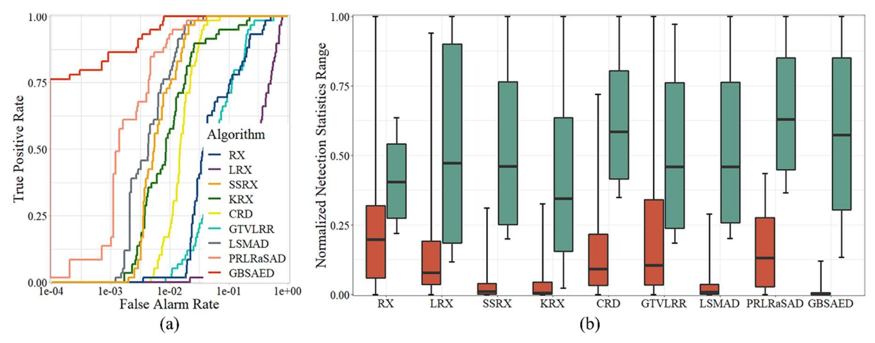
4.3. Detection Performance

Several evaluation indicators were used to evaluate the performance of the nine algorithms described above, including a detection results map, receiver operating characteristic (ROC) curve, normalized target-background separation map, area under the ROC curve (AUC), and running time. Algorithmic detection results maps for the same dataset were obtained in the same stretching mode. ROC curves visualizes the performance of algorithms, with the horizontal axis representing the false alarm rate and the vertical axis representing the detection rate. If a model has good performance, its ROC curve is generally located in the upper left corner of the coordinate plane. Where two or more curves intersect or overlap, comparing the performance of algorithms can be difficult. In such cases, the AUC value can be used to quantitatively analyze the results, where larger AUC values indicate better performance. A target-background separation map divides normalized pixel values into two boxes. The red and green boxes represent the pixel distribution values of background and anomalous pixels. The line in the center of each box represents the median pixel values. The top and bottom borders are the quantiles, representing pixel values of 90 and 10. The two horizontal lines outside the box are extreme pixel values. If a gap is apparent between the two boxes, the detector has good performance in terms of distinguishing background and anomalous pixels.

The proposed algorithm is compared to the eight most advanced algorithms in terms of performance. Algorithmic parameter settings are presented in

Table 1. Parameter settings of various algorithms.

Detector	Parameter	Texas Coast	Belcher Bay	PaviaC	San Diego	Xiong’an
LRX	(Win, Wout)	(19, 21)	(19, 21)	(7, 9)	(11, 25)	(19, 21)
KRX	Wlength	9	9	9	9	5
	Kernel function	Polynomial	Polynomial	Polynomial	Polynomial	Polynomial
	Kernel variance	1	0.6	1.6	0.1	3
CRD	(Win, Wout)	(5, 9)	(15, 17)	(7, 9)	(15, 17)	(15, 17)
GTVLRR	Beta	1000	0.01	1000	0.01	100
	Lambda	0.01	0.01	0.001	0.1	0.1
	Gamma	0.01	0.001	0.01	0.01	0.01
LSMAD	r	1	3	1	2	3
	Card	3	1	1	1	5
	Power	1	9	1	10	1
PRLRaSAD	r	2	2	1	2	2
	Card	0.21	0.25	0.475	0.125	0.272
	a	100	100	100	100	100
GBSAED	r	1	3	1	2	3
	$\lambda$	1	20	1	20	30
	K	1	1	1	10	5
	$\tau$	0.001	0.001	0.001	0.001	0.001
	$∆r$	1	1	1	1	1

. RX and SSRX are excluded from the table because they do not require parameters. The AUC value of each algorithm is listed in

Table 2. AUC values of each algorithm for five datasets.

Detector	Texas Coast	Belcher Bay	PaviaC	San Diego	Xiong’an	Average (All Scenes)
RX	0.9946	0.9617	0.9984	0.9112	0.9026	0.9537
LRX	0.9463	0.9975	0.9430	0.9461	0.9276	0.9521
SSRX	0.9801	0.9723	0.9877	0.9918	0.4482	0.8760
KRX	0.9938	0.9802	0.9993	0.979	0.9469	0.9798
CRD	0.9460	0.9929	0.9894	0.9821	0.9400	0.9701
GTVLRR	0.9799	0.9670	0.9975	0.9090	0.9402	0.9587
LSMAD	0.9988	0.9914	0.9998	0.9936	0.9735	0.9914
PRLRaSAD	0.9978	0.9057	0.9998	0.9964	0.9757	0.9751
GBSAED	0.9993	0.9999	0.9998	0.9993	0.9840	0.9965

, with the maximum values in bold type. The program running time of each algorithm is indicated in

Table 3. Running times of each algorithm for five datasets.

Detector	Texas Coast	Belcher Bay	PaviaC	San Diego	Xiong’an	Average (All Scenes)
RX	0.094	0.154	0.051	0.079	0.138	0.103
LRX	38.937	49.081	8.417	49.263	83.620	45.864
SSRX	0.159	0.232	0.098	0.166	0.208	0.173
KRX	21.751	49.611	19.447	23.059	6.389	24.051
CRD	5.943	17.357	2.618	7.539	12.678	9.227
GTVLRR	127.234	278.054	95.241	96.602	212.809	161.988
LSMAD	8.527	17.018	4.380	7.847	14.190	10.392
PRLRaSAD	15.413	16.428	5.362	9.321	18.952	13.059
GBSAED	0.115	0.243	0.118	0.117	0.165	0.152

.

Figure 5 visualizes the detection results for the Texas Coast Image obtained by each algorithm. As shown in the figure, the RX, LRX, and GTVLRR contained stripes because these methods retain spectral band data with stripe noise. The RX, LRX, and CRD results had numerous major false alarms. The SSRX, LSMAD, and PRLRaSAD results showed good performance, but had poorly restrained backgrounds. KRX had better detection results, but high time cost. GBSAED could restrain the background well and also clearly recognized anomalies. The ROC curves presented in Figure 6a indicate that the proposed GBSAED algorithm performed better performance than the other algorithms. In addition to a low false alarm rate, GBSAED also showed good performance. The box plots presented in Figure 6 show that the GBSAED algorithm is better able to restrain the background, and thus can easily separate background from anomalous pixels. The AUC value of GBSAED was 0.9993, which was higher than the values of all other algorithms tested. Combined with the operation time analysis outlined in Table 3, this result demonstrates that GBSAED is a promising detector with low processing cost.

Figure 7 illustrates the detection results for the Belcher Bay Image. This dataset reflects the disadvantages of sliding window algorithms for processing small-scale, “messy” backgrounds. The LRX, KRX, CRD, and GTVLRR algorithms caused false alarms, in part due to classifying rocks in the water body as anomalies. RX wrongly classified a building with unusual materials and some vegetation as anomalies. The LSMAD and SSRX algorithms showed relatively good results, but had apparent false alarms for vegetation and some buildings. The GBSAED method restrained rocks, vegetation, and buildings and separated the anomalies. As shown in Figure 8a, the ROC curve area of GBSAED was significantly larger than all other curves, indicating a high detection rate and extremely low false alarm rate. Figure 8b illustrates that GBSAED had better restraint performance than the other methods; this method could well-separate background and anomalous pixels. The overlap between the two pixel types was markedly smaller for the other methods. As indicated in Table 2 and Table 3, the AUC value of GBSAED was 0.9993. Even with its low time cost, GBSAED provided better detection results than the other methods.

Figure 9 shows the detection results for the PaviaC Image. RX, LRX, SSRX, and PRLRaSAD detected cars and some bridge pixels as anomalies, leading to false alarms. LSMAD and GTVLRR were better at restraining the background, but false alarms also arose at the edge of the bridge. LRX and CRD classified some water body pixels as anomalies. Moreover, the overall images showed apparent noise. KRX had relatively good performance, but its operation time was high, reaching 19.447 s. Overall, GBSAED was the best method. The ROC curve analysis demonstrated its superior performance, as shown in Figure 10a. Figure 10b shows a large gap between the background box and anomaly box in the GBSAED method, indicating that this method provided good separation, and its background was restrained at a lower level. The AUC value of GBSAED was 0.9998, and its run time was 0.118 s. Thus, the GBSAED method achieved fast and accurate anomaly detection.

Figure 11 shows the detection results for the San Diego Image. As the image contained sparse background pixels in the lower-left and upper-left corners, its background components were relatively complex. As shown in Figure 11, the RX method had difficulty identifying anomalies and classified many background materials as anomalies. LRX and GTVLRR filtered out some false alarms, but also showed poor detection of real anomalies. LRX also requires a large window to traverse, which increases its time cost considerably. KRX, CRD, LSMAD, and PRLRaSAD successfully detected anomalies, but also had many false alarms. GBSAED had the best background suppression and high operating efficiency. As shown in Figure 12a, the ROC curve of GBSAED leveled off toward the upper left corner and the area was larger than that under the other curves. As shown in Figure 12b, a gap was present between the background and anomaly boxes, indicating that separation performance was good. The AUC value of GBSAED was 0.9993. GBSAED’s run time was only 0.117 s, compared to 49.263 s for LRX. From the perspectives of both qualitative and quantitative analysis, GBSAED showed relatively good performance.

Figure 13 visualizes the detection results for the Xiong’an Image. The image quality significantly influenced RX, LRX, and CRD, and their results maps contained many noise stripes, which greatly affected the results and complex anomaly detection performance. In contrast to other datasets, for the Xiong’an Image, SSRX classified cars as background but classified some vegetation pixels as anomalies. This misclassification indicates that SSRX cannot be applied to all image types. In the detection results of the PRLRaSAD algorithm, the yellow line was brighter than the cars, and large areas of the road caused false alarms. The LSMAD and GTVLRR algorithm had relatively good results, but still produced a false alarm for the yellow line. The overall performance of the KRX algorithm was good, but it was also time-consuming. The GBSAED algorithm precisely detected all anomalies and had the fewest false alarms. Therefore, GBSAED was the best-performing method. Figure 14a,b qualitatively show the performance of GBSAED, which was characterized by a high detection rate, strong restraint of the background, and low false alarm rate. The AUC value of GBSAED was 0.9840 and the run time was 0.165 s; KRX had similarly excellent test results but required 6.389 s to run.

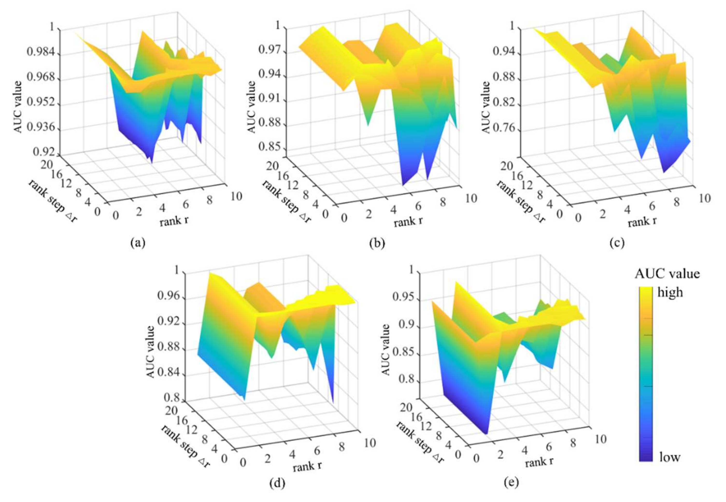
4.4. Parameter Setting Considerations

The GBSAED algorithm has four important parameters: rank r, rank step, $∆r$ soft thresholding $\lambda$, and power K. In this section, all other parameters were set to their default values and thus not optimized. The default value for tolerance $\tau$ was 0.001. Aside from rank, all other default values were set to 1.

Rank is one of the most critical parameters and it is generally believed that the optimal rank value is correlated with the number of irrelevant components in the background. Thus, the rank value depends on the number of predominant background objects. Meanwhile, the optimal rank value is often the minimum value. In this study, the rank values were based on the colors of the first three principal components within the HSI data, as shown in Figure 15. Less strongly correlated components in the background were represented as high-contrast colors. For the Texas Coast Image and PaviaC Image, which have simple backgrounds, the rank value was set to 1. For the San Diego Image with two main materials as the background, the rank parameter was set to 2. For the Belcher Bay Image with a background of buildings, vegetation, and water, and the Xiong’an Image with vegetation, road, and a yellow line in the background, the rank value was set to 3.

Figure 16 shows changes in AUC values according to the values of r and $∆r$. Generally speaking, lower $∆r$ values indicate higher detection precision. As $∆r$ rises, the operation time of some HSI algorithms decreases significantly. For HSI data with a relatively simple background where r = 1, the AUC values shows no apparent change according to $∆r$, and the efficiency also changes little. For HSI data with a relatively complex background, where r≥2, assuming the other parameters are set properly, efficiency will improve significantly as $∆r$ rises, thereby providing stable and correct detection results. For tasks with complex backgrounds that require high precision, a smaller $∆r$ value may improve detection. In this study, the $∆r$ values of all five datasets were set to the minimum value of 1.

For the three-dimensional AUC values of $\lambda$ and r, there is a clear rule within a small threshold range of $\lambda$, indicated in Figure 17 by a plane that does not change with changes in $\lambda$. Thus, within a small range of $\lambda$, the AUC value changes only with r, leading to high and stable detection accuracy. A method with these characteristics is applicable to HSIs with relatively simple backgrounds, such as the Texas Coast Image, PaviaC Image, and other application scenarios that require fast detection. Furthermore, changes in $\lambda$ have relatively little influence on precision when rank is set to the optimal value.

For analysis of complex backgrounds, the values of $\lambda$ and K can be increased to improve detection accuracy. Figure 18 presents AUC values according to changes in $\lambda$ and K. For the Belcher Bay Image, San Diego Image, and Xiong’an Image, with r ≥ 2, as the two parameters increase, the AUC value increases gradually and then stabilizes. Notably, for the Texas Coast Image and PaviaC Image, with r = 1, the opposite trend occurs. Thus, for HSI data with a relatively simple background, increasing the values of these two parameters may slightly reduce detection accuracy. Therefore, smaller parameter values should be selected for such images.

5. Conclusions

This study introduces a fast hyperspectral anomaly detection algorithm based on the GBSAED method, with the aims of improving detection performance under conditions in which the background and anomalies of similar components are difficult to separate, and reducing the high time cost associated with the LRaSMD algorithm. In this study, the EMAP method was used to restrain the background and reduce false alarms. A greedy bilateral smoothing method was employed to detect spectral anomalies, which greatly improved the operational efficiency. A series of experiments using five real hyperspectral datasets with differences in image quality, spatial resolution, spectral resolution, and anomaly distribution characteristics demonstrated the robustness of the proposed algorithm. In a comparison of the RX, LRX, SSRX, KRX, CRD, GTVLRR, LSMAD and PRLRaSAD detectors, the GBSAED method showed the best performance. This method increased the average AUC values of the five datasets by 4.276%, 4.436%, 12.044%, 1.662%, 2.638%, 3.775%, 0.504%, and 2.139%. In addition, it reduced run time, with an average run time for all datasets of 0.152 s, which was second only to 0.103 s for RX. Through full analysis of the parameters of the proposed algorithm, clear rules for the parameter settings of the GBSAED algorithm were determined for various types of datasets. Overall, the GBSAED algorithm offers improved performance and increased operational efficiency for HSI anomaly detection.

GBSAED algorithm has a better performance in processing anomalies with spatial characteristics rather than dealing with subpixels. Therefore, our further direction will focus on the adaptability improvement of the algorithm.

References

1. Bioucas-Dias, J.M.; Plaza, A.; Camps-Valls, G.; Scheunders, P.; Nasrabadi, N.; Chanussot, J. Hyperspectral Remote Sensing Data Analysis and Future Challenges. IEEE Geosci. Remote Sens. Mag. 2013, 1, 6–36. [Google Scholar] [CrossRef] [Green Version]
2. Stein, D.; Beaven, S.G.; Hoff, L.E.; Winter, E.M.; Stocker, A.D. Anomaly detection from hyperspectral imagery. IEEE Signal Process. Mag. 2002, 19, 58–69. [Google Scholar] [CrossRef] [Green Version]
3. Plaza, A.; Benediktsson, J.A.; Boardman, J.W.; Brazile, J.; Bruzzone, L.; Camps-Valls, G.; Chanussot, J.; Fauvel, M.; Gamba, P.; Gualtieri, A.; et al. Recent advances in techniques for hyperspectral image processing. Remote Sens. Environ. 2009, 113, S110–S122. [Google Scholar] [CrossRef]
4. Zhang, Y.; Fan, Y.; Xu, M.; Li, W.; Zhang, G.; Liu, L.; Yu, D. An Improved Low Rank and Sparse Matrix Decomposition-Based Anomaly Target Detection Algorithm for Hyperspectral Imagery. IEEE J. Sel. Top. Appl. Earth Obs. Remote Sens. 2020, 13, 2663–2672. [Google Scholar] [CrossRef]
5. Chang, C.I.; Chiang, S.S. Anomaly detection and classification for hyperspectral imagery. IEEE Trans. Geosci. Remote Sens. 2002, 40, 1314–1325. [Google Scholar] [CrossRef] [Green Version]
6. Nasrabadi, N. Hyperspectral Target Detection: An Overview of Current and Future Challenges. IEEE Signal Process. Mag. 2013, 31, 34–44. [Google Scholar] [CrossRef]
7. Jia, S.; Deng, X.; Zhu, J.; Xu, M.; Zhou, J.; Jia, X. Collaborative Representation-Based Multiscale Superpixel Fusion for Hyperspectral Image Classification. IEEE Trans. Geosci. Remote Senss. 2019, 57, 7770–7784. [Google Scholar] [CrossRef]
8. Yang, W.; Peng, J.; Sun, W.; Du, Q. Log-Euclidean Kernel-Based Joint Sparse Representation for Hyperspectral Image Classification. IEEE J. Sel. Top. Appl. Earth Obs. Remote Sens. 2020, 12, 5023–5034. [Google Scholar] [CrossRef]
9. Zhang, Y.; Fan, Y.; Xu, M. A Background-Purification-Based Framework for Anomaly Target Detection in Hyperspectral Imagery. IEEE Geosci. Remote Sens. Lett. 2019, 17, 1–5. [Google Scholar] [CrossRef]
10. Manolakis, D.; Truslow, E.; Pieper, M.; Cooley, T. Detection Algorithms in Hyperspectral Imaging Systems: An Overview of Practical Algorithms. IEEE Signal Process. Mag. 2014, 31, 24–33. [Google Scholar] [CrossRef]
11. Eismann, M.T.; Stocker, A.D.; Nasrabadi, N.M. Automated Hyperspectral Cueing for Civilian Search and Rescue. Proc. IEEE 2009, 97, 1031–1055. [Google Scholar] [CrossRef]
12. Ma, D.; Yuan, Y.; Wang, Q. Hyperspectral Anomaly Detection Based on Separability-Aware Sample Cascade. Remote Sens. 2019, 11, 2537. [Google Scholar] [CrossRef] [Green Version]
13. Li, Z.; Zhang, Y. A New Hyperspectral Anomaly Detection Method Based on Higher Order Statistics and Adaptive Cosine Estimator. IEEE Geosci. Remote Sens. Lett. 2019, 17, 1–5. [Google Scholar] [CrossRef]
14. Cheng, T.; Wang, B. Graph and Total Variation Regularized Low-Rank Representation for Hyperspectral Anomaly Detection. IEEE Trans. Geosci. Remote Sens. 2020, 58, 391–406. [Google Scholar] [CrossRef]
15. Taghipour, A.; Ghassemian, H. Visual attention-driven framework to incorporate spatial-spectral features for hyperspectral anomaly detection. Int. J. Remote Sens. 2021, 42, 7454–7488. [Google Scholar] [CrossRef]
16. Li, L.; Li, W.; Du, Q.; Tao, R. Low-Rank and Sparse Decomposition With Mixture of Gaussian for Hyperspectral Anomaly Detection. IEEE Trans. Cybern. 2021, 51, 4363–4372. [Google Scholar] [CrossRef]
17. Ma, Y.; Fan, G.H.; Jin, Q.W.; Huang, J.; Mei, X.G.; Ma, J.Y. Hyperspectral Anomaly Detection via Integration of Feature Extraction and Background Purification. IEEE Geosci. Remote Sens. Lett. 2021, 18, 1436–1440. [Google Scholar] [CrossRef]
18. Huang, Z.; Kang, X.; Li, S.; Hao, Q. Game Theory-Based Hyperspectral Anomaly Detection. IEEE Trans. Geosci. Remote Sens. 2019, 58, 1–12. [Google Scholar] [CrossRef]
19. Reed, I.S.; Yu, X. Adaptive multiple-band CFAR detection of an optical pattern with unknown spectral distribution. IEEE Trans. Acoust. Speech Signal Process. 1990, 38, 1760–1770. [Google Scholar] [CrossRef]
20. Schaum, A. Joint Subspace Detection of hyperspectral targets. In Proceedings of the IEEE Aerospace Conference 2004, Big Sky, MT, USA, 6–13 March 2004. [Google Scholar]
21. Nasrabadi, N.M. Regularization for spectral matched filter and RX anomaly detector. In Proceedings of the Conference on Algorithms and Technologies for Multispectral, Hyperspectral, and Ultraspectral Imagery, Orlando, FL, USA, 11 April 2008. [Google Scholar]
22. Kwon, H.; Nasrabadi, N.M. Kernel RX-algorithm: A nonlinear anomaly detector for hyperspectral imagery. IEEE Trans. Geosci. Remote Sens. 2005, 43, 388–397. [Google Scholar] [CrossRef]
23. Zhou, J.; Kwan, C.; Ayhan, B.; Eismann, M.T. A Novel Cluster Kernel RX Algorithm for Anomaly and Change Detection Using Hyperspectral Images. IEEE Trans. Geosci. Remote Sens. 2016, 54, 6497–6504. [Google Scholar] [CrossRef]
24. Carlotto, M.J. A cluster-based approach for detecting man-made objects and changes in imagery. IEEE Trans. Geosci. Remote Sens. 2005, 43, 374–387. [Google Scholar] [CrossRef]
25. Guo, Q.; Zhang, B.; Ran, Q.; Gao, L.; Li, J.; Plaza, A. Weighted-RXD and Linear Filter-Based RXD: Improving Background Statistics Estimation for Anomaly Detection in Hyperspectral Imagery. IEEE J. Sel. Top. Appl. Earth Obs. Remote Sens. 2014, 7, 2351–2366. [Google Scholar] [CrossRef]
26. Billor, N.; Hadi, A.S.; Velleman, P.F. BACON: Blocked adaptive computationally efficient outlier nominators. Comput. Stat. Data Anal. 2000, 34, 279–298. [Google Scholar] [CrossRef]
27. Li, W.; Du, Q. Collaborative Representation for Hyperspectral Anomaly Detection. IEEE Trans. Geosci. Remote Sens. 2015, 53, 1463–1474. [Google Scholar] [CrossRef]
28. Li, J.; Zhang, H.; Zhang, L.; Ma, L. Hyperspectral Anomaly Detection by the Use of Background Joint Sparse Representation. IEEE J. Sel. Top. Appl. Earth Obs. Remote Sens. 2015, 8, 2523–2533. [Google Scholar] [CrossRef]
29. Yang, X.; Wu, Z.; Li, J.; Plaza, A.; Wei, Z. Anomaly Detection in Hyperspectral Images Based on Low-Rank and Sparse Representation. IEEE Trans. Geosci. Remote Sens. 2016, 54, 1990–2000. [Google Scholar]
30. Rui, Z.; Bo, D.; Zhang, L. Hyperspectral Anomaly Detection via A Sparsity Score Estimation Framework. IEEE Trans. Geosci. Remote Sens. 2017, 55, 3208–3222. [Google Scholar]
31. Ling, Q.; Guo, Y.; Lin, Z.; An, W. A Constrained Sparse Representation Model for Hyperspectral Anomaly Detection. IEEE Trans. Geosci. Remote Sens. 2018, 57, 1–14. [Google Scholar] [CrossRef]
32. Vafadar, M.; Ghassemian, H. Anomaly Detection of Hyperspectral Imagery Using Modified Collaborative Representation. IEEE Geosci. Remote Sens. Lett. 2018, 15, 1–5. [Google Scholar] [CrossRef]
33. Xi, C.; Liang, X.; Schneider, J. direct robust matrix factorizatoin for anomaly detection. In Proceedings of the 11th IEEE International Conference on Data Mining, ICDM 2011, Vancouver, BC, Canada, 11–14 December 2011. [Google Scholar]
34. Sun, W.; Liu, C.; Li, J.; Lai, Y.M.; Li, W. Low-rank and sparse matrix decomposition-based anomaly detection for hyperspectral imagery. J. Appl. Remote Sens. 2014, 8, 083641. [Google Scholar] [CrossRef]
35. Cui, X.; Yuan, T.; Weng, L.; Yang, Y. Anomaly detection in hyperspectral imagery based on low-rank and sparse decomposition. Int. Soc. Opt. Photonics 2014, 9069. [Google Scholar] [CrossRef]
36. Zhang, Y.X.; Du, B.; Zhang, L.P.; Wang, S.G. A Low-Rank and Sparse Matrix Decomposition-Based Mahalanobis Distance Method for Hyperspectral Anomaly Detection. IEEE Trans. Geosci. Remote Sens. 2016, 54, 1376–1389. [Google Scholar] [CrossRef]
37. Yang, Y.; Zhang, J.; Song, S.; Zhang, C.; Liu, D. Low-Rank and Sparse Matrix Decomposition with Orthogonal Subspace Projection-Based Background Suppression for Hyperspectral Anomaly Detection. IEEE Geosci. Remote Sens. Lett. 2019, 17, 1–5. [Google Scholar] [CrossRef]
38. Zhu, L.; Wen, G.; Qiu, S. Low-Rank and Sparse Matrix Decomposition with Cluster Weighting for Hyperspectral Anomaly Detection. Remote Sens. 2018, 10, 707. [Google Scholar] [CrossRef] [Green Version]
39. Zhang, H.; Wei, H.; Zhang, L.; Shen, H.; Yuan, Q. Hyperspectral Image Restoration Using Low-Rank Matrix Recovery. IEEE Trans. Geosci. Remote Sens. 2014, 52, 4729–4743. [Google Scholar] [CrossRef]
40. Zhou, T.; Tao, D. GoDec: Randomized low-rank & sparse matrix decomposition in noisy case. In Proceedings of Proceedings of the 28th International Conference on International Conference on Machine Learning, Bellevue, WA, USA, 28 June–2 July 2011; pp. 33–40. [Google Scholar]
41. Pesaresi, M.; Benediktsson, J.A. A new approach for the morphological segmentation of high-resolution satellite imagery. IEEE Trans. Geosci. Remote Sens. 2002, 39, 309–320. [Google Scholar] [CrossRef] [Green Version]
42. Dalla Mura, M.; Atli Benediktsson, J.; Waske, B.; Bruzzone, L. Extended profiles with morphological attribute filters for the analysis of hyperspectral data. Int. J. Remote Sens. 2010, 31, 5975–5991. [Google Scholar] [CrossRef]
43. Mura, D.; Benediktsson, M.; Atli, J.; Bjrn, W.; Bruzzone, L. Morphological Attribute Profiles for the Analysis of Very High Resolution Images. IEEE Trans. Geosci. Remote Sens. 2010, 48, 3747–3762. [Google Scholar] [CrossRef]
44. Zhou, T.; Tao, D. Greedy Bilateral Sketch, Completion & Smoothing. JMLR ORG 2013, 31, 650–658. [Google Scholar]
45. Kang, X.; Zhang, X.; Li, S.; Li, K.; Li, J.; Benediktsson, J.A. Hyperspectral Anomaly Detection With Attribute and Edge-Preserving Filters. IEEE Trans. Geosci. Remote Sens. 2017, 55, 5600–5611. [Google Scholar] [CrossRef]
Figure 1. Flowchart of the GBSAED method.
Remotesensing 13 03954 g001
Figure 2. EMAP maps of the four attributes: (a) EMAPa, (b) EMAPd, (c) EMAPi, (d) EMAPs.
Remotesensing 13 03954 g002
Figure 3. Detection details for spatial, spectral, and GBSAED methods. (A) Sparse background area A, (B) Sparse background area B, (C) Sparse background area C.
Remotesensing 13 03954 g003
Figure 4. False-color composite images and ground truth maps of the five datasets used: (a) Texas Coast Image, (b) Belcher Bay Image, (c) PaviaC Image, (d) San Diego Image, and (e) Xiong’an Image.
Remotesensing 13 03954 g004
Figure 5. Detection results of the various algorithms for the Texas Coast Image: (a) RX, (b) LRX, (c) KRX, (d) SSRX, (e) CRD, (f) LSMAD, (g) GTVLRR, (h) PRLRaSAD, and (i) GBSAED.
Remotesensing 13 03954 g005
Figure 6. Quantitative analysis of the detection results of the various algorithms for the Texas Coast Image: (a) ROC curves and (b) target-background separation map.
Remotesensing 13 03954 g006
Figure 7. Detection results of the various algorithms for the Belcher Bay Image: (a) RX, (b) LRX, (c) KRX, (d) SSRX, (e) CRD, (f) LSMAD, (g) GTVLRR, (h) PRLRaSAD, and (i) GBSAED.
Remotesensing 13 03954 g007
Figure 8. Quantitative analysis of the detection results of the various algorithms for the Belcher Bay Image: (a) ROC curves and (b) target-background separation map.
Remotesensing 13 03954 g008
Figure 9. Detection results of various algorithms for the PaviaC Image: (a) RX, (b) LRX, (c) KRX, (d) SSRX, (e) CRD, (f) LSMAD, (g) GTVLRR, (h) PRLRaSAD, and (i) GBSAED.
Remotesensing 13 03954 g009
Figure 10. Quantitative analysis of the detection results of the various algorithms for the PaviaC Image: (a) ROC curves and (b) target-background separation map.
Remotesensing 13 03954 g010
Figure 11. Detection results of the various algorithms for the San Diego Image: (a) RX, (b) LRX, (c) KRX, (d) SSRX, (e) CRD, (f) LSMAD, (g) GTVLRR, (h) PRLRaSAD, and (i) GBSAED.
Remotesensing 13 03954 g011
Figure 12. Quantitative analysis of the detection results of the various algorithms for the San Diego Image: (a) ROC curves and (b) target-background separation map.
Remotesensing 13 03954 g012
Figure 13. Detection results of the various algorithms for the Xiong’an Image: (a) RX, (b) LRX, (c) KRX, (d) SSRX, (e) CRD, (f) LSMAD, (g) GTVLRR, (h) PRLRaSAD, and (i) GBSAED.
Remotesensing 13 03954 g013
Figure 14. Quantitative analysis of the detection results of the various algorithms for the Xiong’an Image: (a) ROC curves and (b) target-background separation map.
Remotesensing 13 03954 g014
Figure 15. Color composite images of the first three principal components of the HSI images: (a) Texas Coast Image, (b) Belcher Bay Image, (c) PaviaC Image, (d) San Diego Image, and (e) Xiong’an Image.
Remotesensing 13 03954 g015
Figure 16. AUC values of GBSAED according to changes in rank step r and rank r: (a) Texas Coast Image, (b) Belcher Bay Image, (c) PaviaC Image, (d) San Diego Image, and (e) Xiong’an Image.
Remotesensing 13 03954 g016
Figure 17. AUC values of GBSAED according to changes in soft thresholding λ and rank r: (a) Texas Coast Image, (b) Belcher Bay Image, (c) PaviaC Image, (d) San Diego Image, and (e) Xiong’an Image.
Remotesensing 13 03954 g017
Figure 18. AUC values of GBSAED according to changes in soft thresholding λ and power K: (a) Texas Coast Image, (b) Belcher Bay Image, (c) PaviaC Image, (d) San Diego Image, and (e) Xiong’an Image.
Remotesensing 13 03954 g018