Impact of Monsoon-Transported Anthropogenic Aerosols and Sun-Glint on the Satellite-Derived Spectral Remote Sensing Reflectance in the Indian Ocean

Abstract
:
1. Introduction
2. Data and Methods
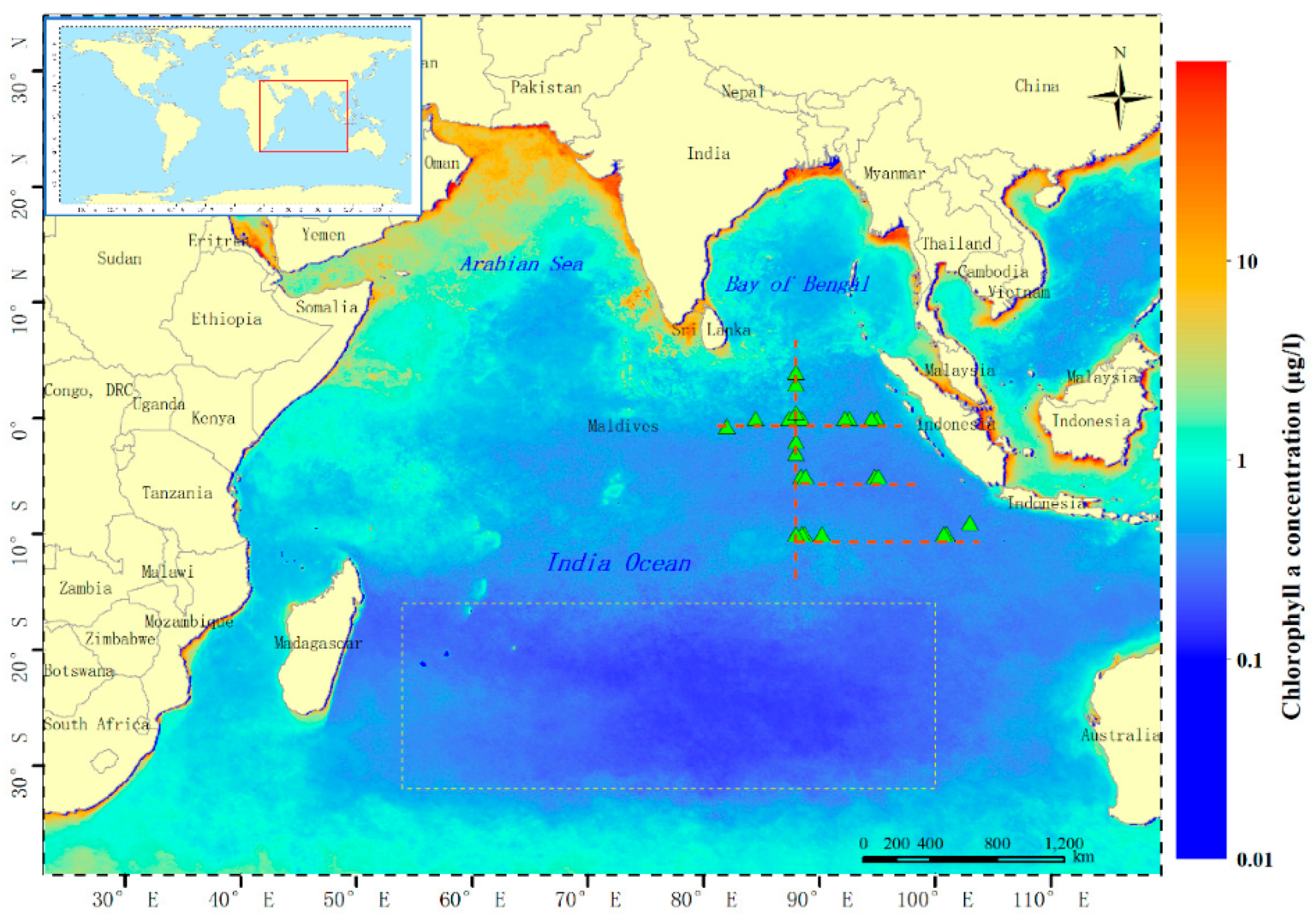
2.1. Study Area
2.2. In Situ Data
2.3. Satellite Data
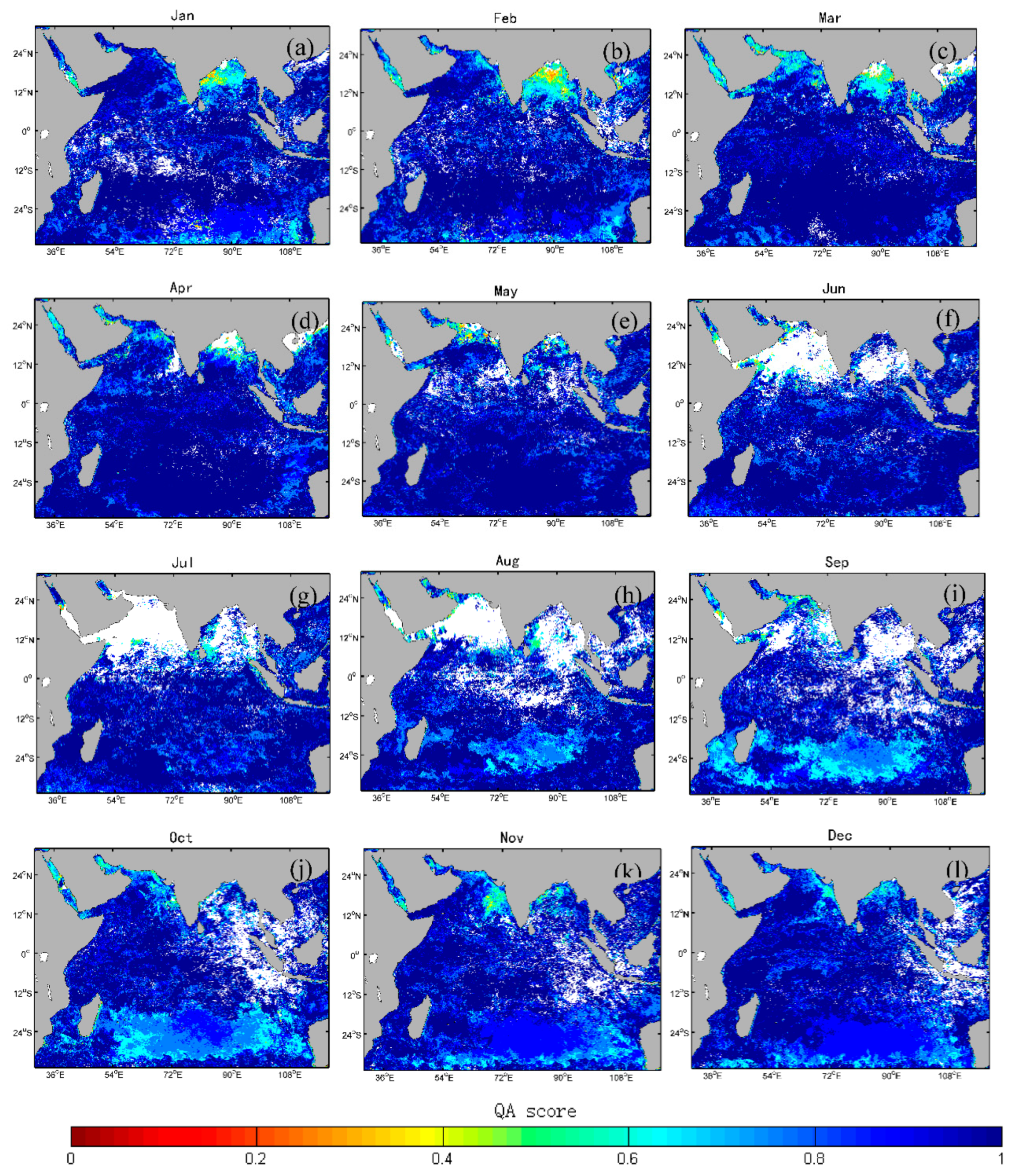
2.4. QA Method
3. Results
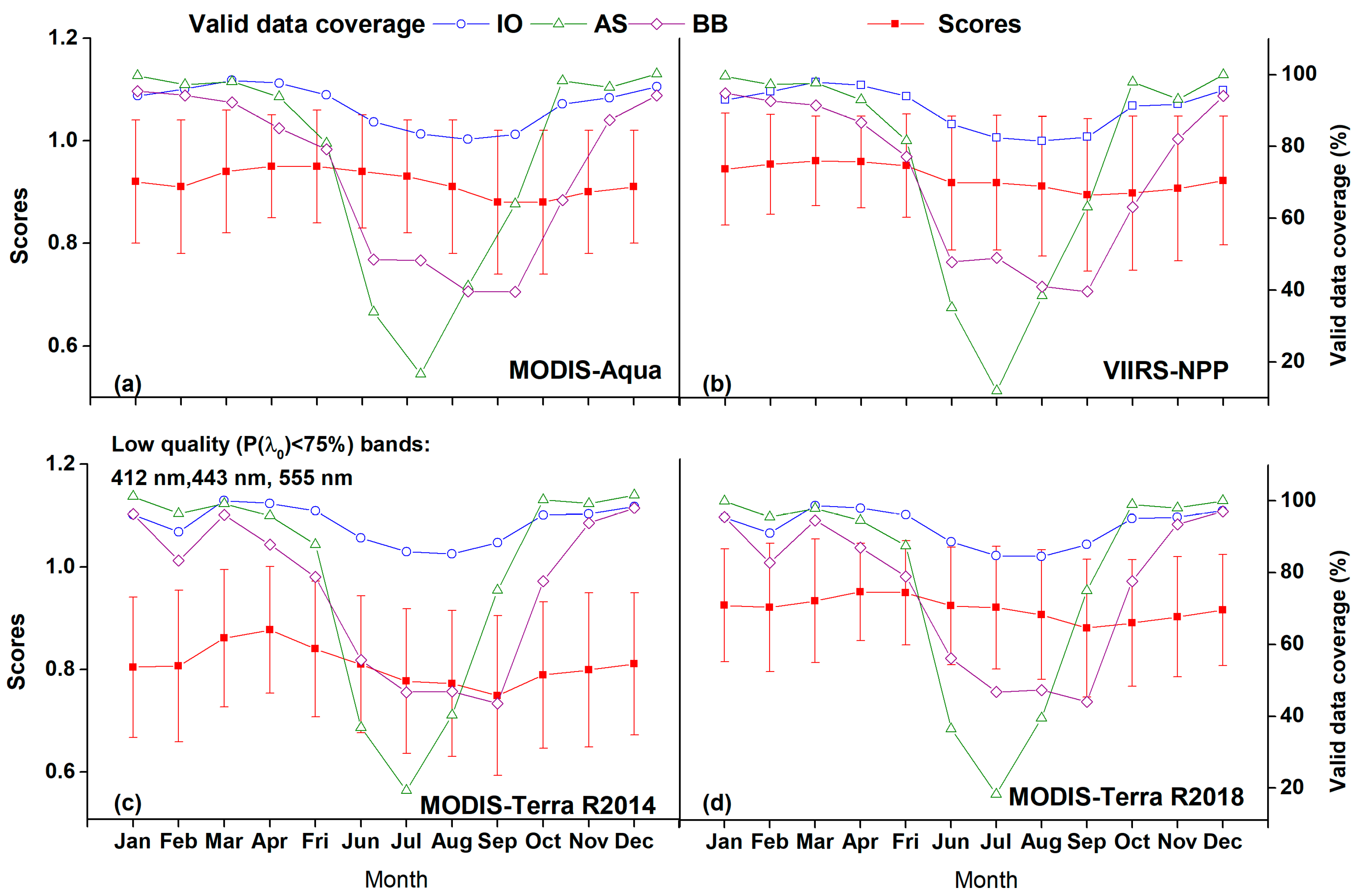
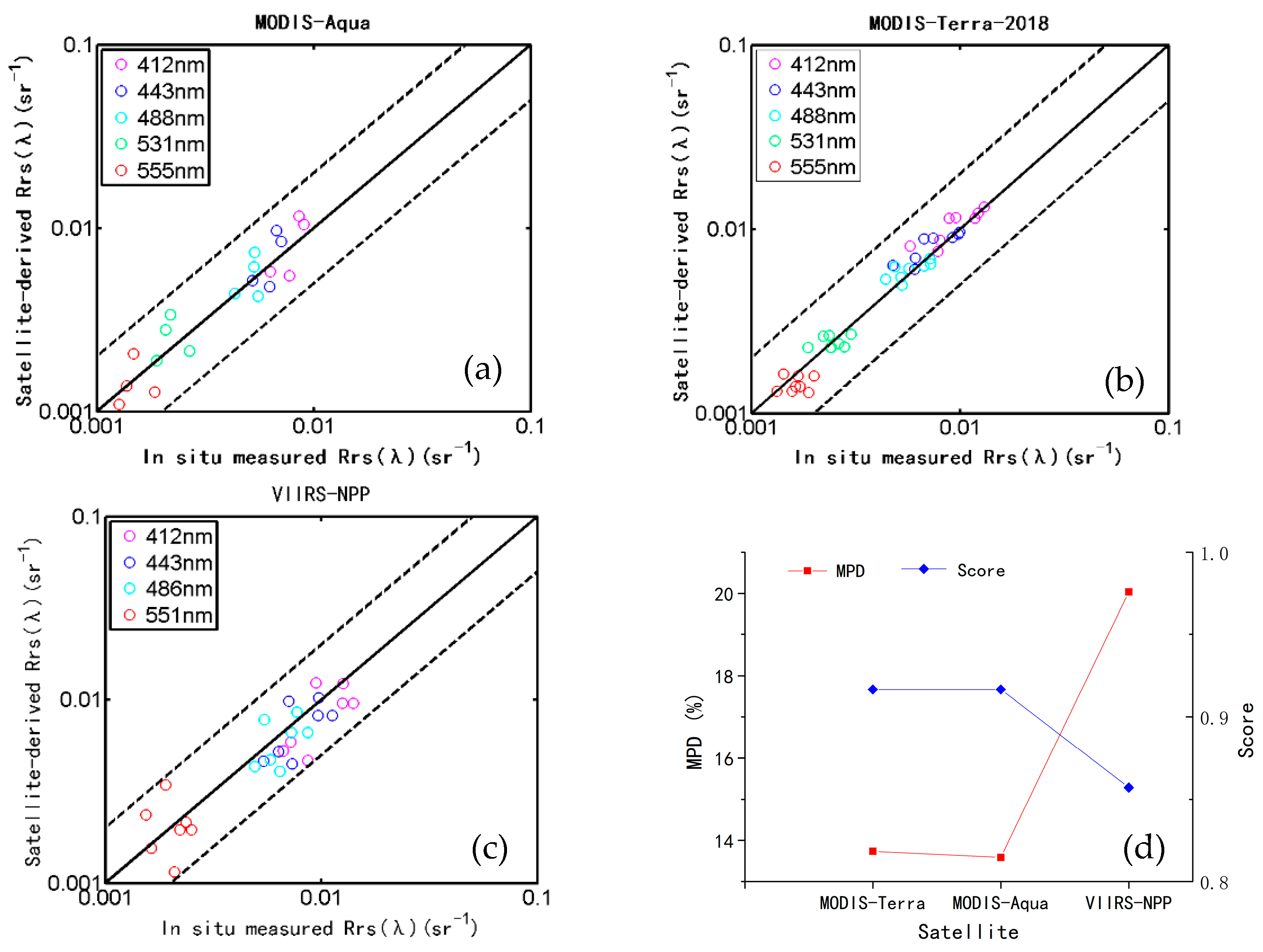
3.1. Validation Results
- (1)
- MODIS-Aqua
- (2)
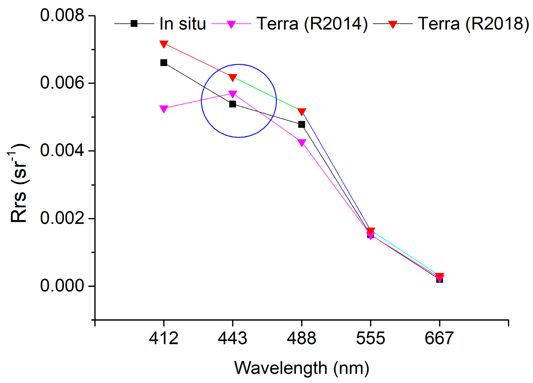
- MODIS-Terra
- (3)
- VIIRS-NPP
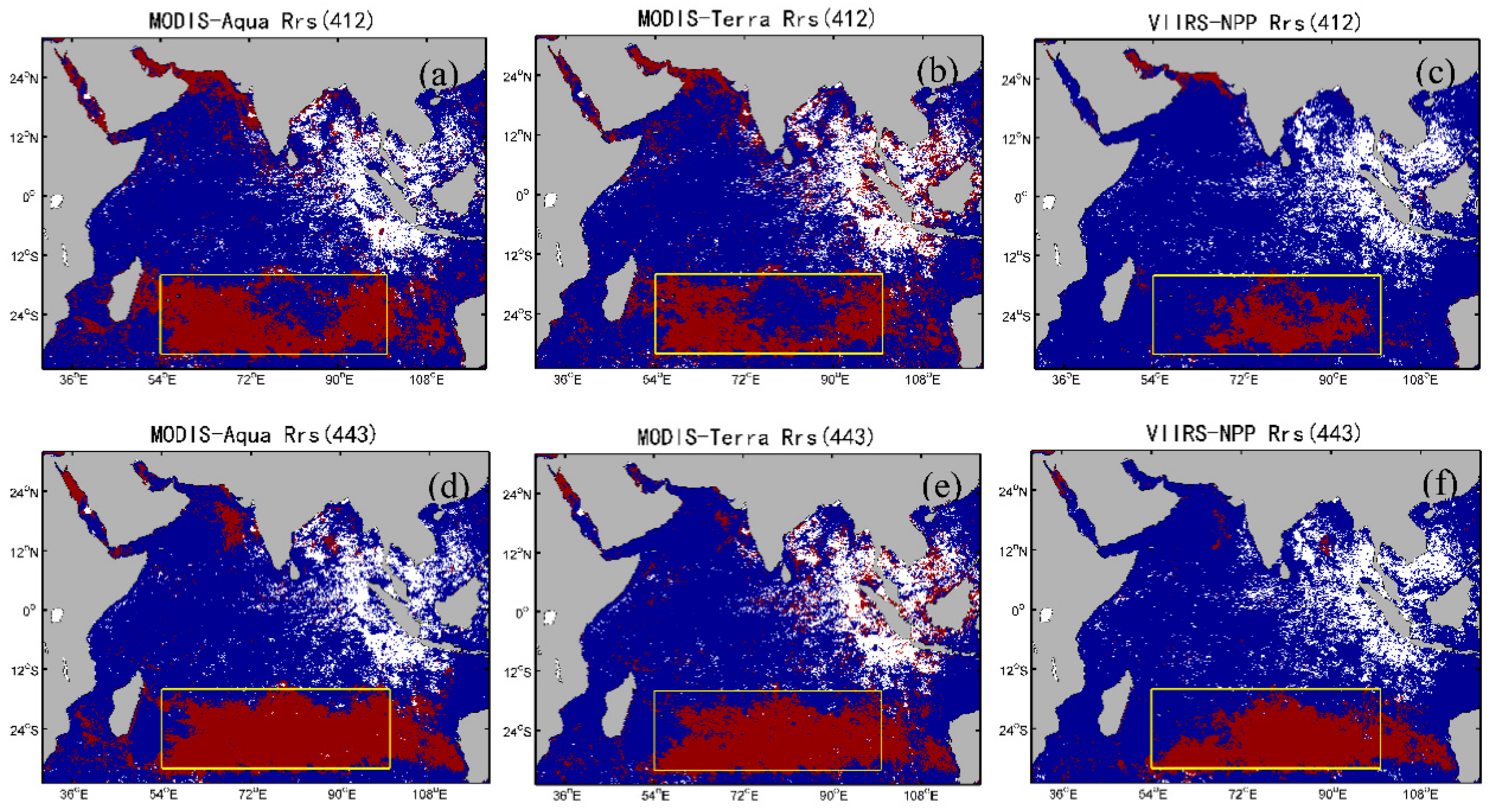
3.2. Mechanisms of Rrs(λ) Quality Spatiotemporal Distribution
3.2.1. Monsoon in the Northern IO
3.2.2. Sun Glint in the OZ
4. Discussion
4.1. QA Analysis
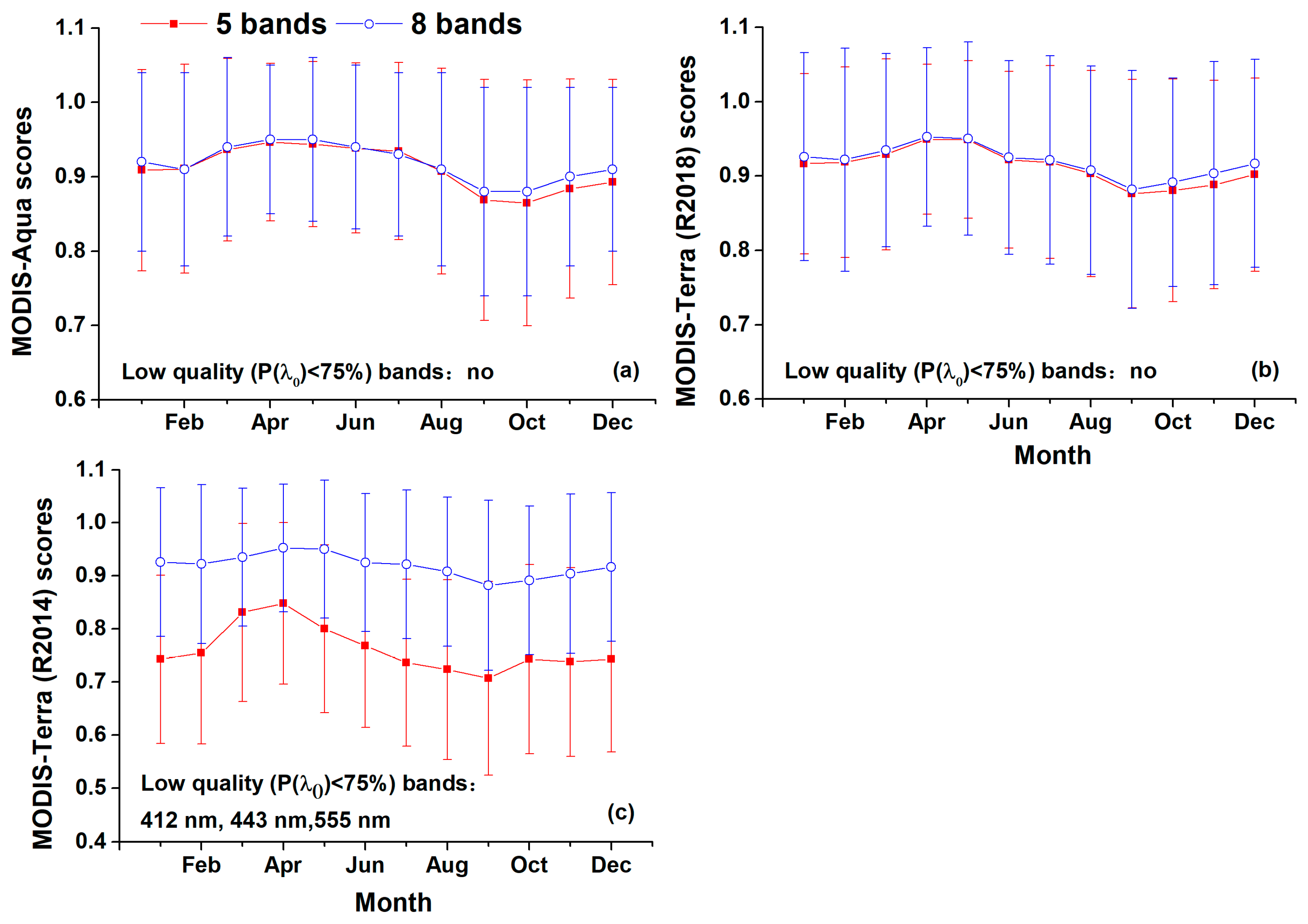
4.1.1. Bands Involved in QA Analysis
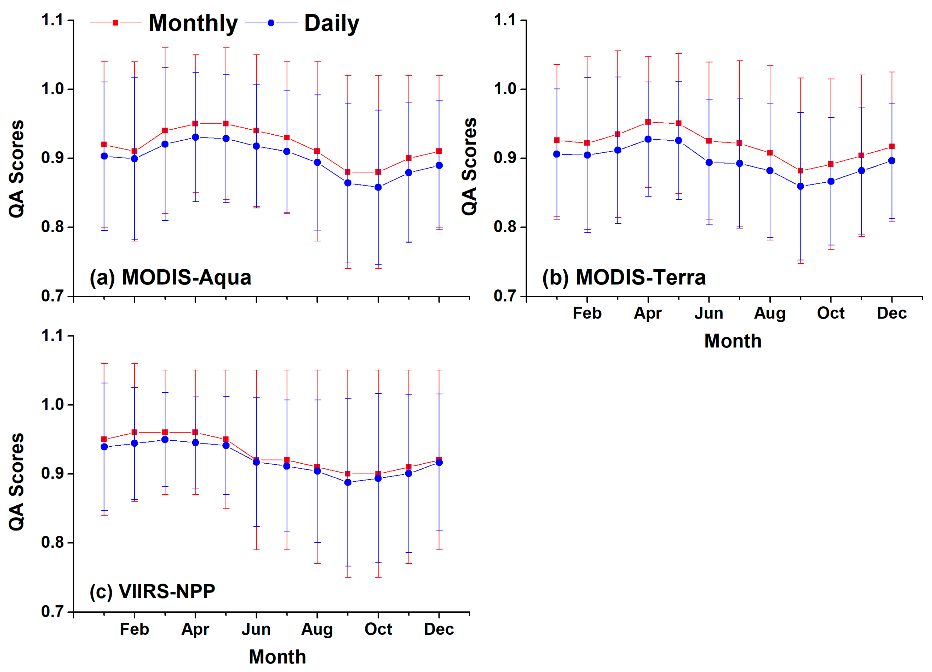
4.1.2. Daily vs. Monthly Products
4.2. Comparison between Results from In Situ-Based and QA Methods
4.3. Implications
5. Conclusions
Author Contributions
Funding
Institutional Review Board Statement
Informed Consent Statement
Data Availability Statement
Acknowledgments
Conflicts of Interest
References
- Ford, D.; Barciela, R. Global marine biogeochemical reanalyses assimilating two different sets of merged ocean colour products. Remote Sens. Environ. 2017, 203, 40–54. [Google Scholar] [CrossRef]
- Le, C.; Zhou, X.; Hu, C.; Lee, Z.; Li, L.; Stramski, D. A Color-Index-Based Empirical Algorithm for Determining Particulate Organic Carbon Concentration in the Ocean from Satellite Observations. J. Geophys. Res. Oceans 2018, 123, 7407–7419. [Google Scholar] [CrossRef]
- Li, J.; Yu, Q.; Tian, Y.Q.; Becker, B.L. Remote sensing estimation of colored dissolved organic matter (CDOM) in optically shallow waters. ISPRS J. Photogramm. Remote Sens. 2017, 128, 98–110. [Google Scholar] [CrossRef] [Green Version]
- Reygondeau, G.; Longhurst, A.R.; Martinez, E.; Beaugrand, G.; Antoine, D.; Maury, O. Dynamic biogeochemical provinces in the global ocean. Glob. Biogeochem. Cycles 2013, 27, 1046–1058. [Google Scholar] [CrossRef] [Green Version]
- Feng, L.; Hou, X.; Zheng, Y. Monitoring and understanding the water transparency changes of fifty large lakes on the Yangtze Plain based on long-term MODIS observations. Remote Sens. Environ. 2019, 221, 675–686. [Google Scholar] [CrossRef]
- Hakvoort, H.; De Haan, J.; Jordans, R.; Vos, R.; Peters, S.; Rijkeboer, M. Towards airborne remote sensing of water quality in The Netherlands—validation and error analysis. ISPRS J. Photogramm. Remote Sens. 2002, 57, 171–183. [Google Scholar] [CrossRef]
- Salama, M.S.; Verhoef, W. Two-stream remote sensing model for water quality mapping: 2SeaColor. Remote Sens. Environ. 2015, 157, 111–122. [Google Scholar] [CrossRef] [Green Version]
- Dutkiewicz, S.; Hickman, A.E.; Jahn, O.; Henson, S.; Beaulieu, C.; Monier, E. Ocean colour signature of climate change. Nat. Commun. 2019, 10, 1–13. [Google Scholar] [CrossRef] [Green Version]
- Montes-Hugo, M.; Doney, S.C.; Ducklow, H.W.; Fraser, W.; Martinson, D.; Stammerjohn, S.E.; Schofield, O. Recent changes in phytoplankton communities associated with rapid regional climate change along the western Antarctic Penin-sula. Science 2009, 323, 1470–1473. [Google Scholar] [CrossRef]
- Sathyendranath, S.; Brewin, R.J.; Jackson, T.; Mélin, F.; Platt, T. Ocean-colour products for climate-change studies: What are their ideal characteristics? Remote Sens. Environ. 2017, 203, 125–138. [Google Scholar] [CrossRef] [Green Version]
- Lee, Z.; Shang, S.; Wang, Y.; Wei, J.; Ishizaka, J. Nature of optical products inverted semianalytically from remote sensing reflectance of stratified waters. Limnol. Oceanogr. 2020, 65, 387–400. [Google Scholar] [CrossRef]
- O’Reilly, J.E.; Werdell, P.J. Chlorophyll algorithms for ocean color sensors—OC4, OC5; OC6. Remote Sens. Environ. 2019, 229, 32–47. [Google Scholar] [CrossRef]
- Bailey, S.W.; Werdell, P.J. A multi-sensor approach for the on-orbit validation of ocean color satellite data products. Remote Sens. Environ. 2006, 102, 12–23. [Google Scholar] [CrossRef]
- Hu, C.; Feng, L.; Lee, Z. Uncertainties of SeaWiFS and MODIS remote sensing reflectance: Implications from clear water measurements. Remote Sens. Environ. 2013, 133, 168–182. [Google Scholar] [CrossRef]
- Moore, T.S.; Campbell, J.W.; Feng, H. Characterizing the uncertainties in spectral remote sensing reflectance for SeaWiFS and MODIS-Aqua based on global in situ matchup data sets. Remote Sens. Environ. 2015, 159, 14–27. [Google Scholar] [CrossRef]
- Zibordi, G.; Mélin, F.; Berthon, J.-F. A Regional Assessment of OLCI Data Products. IEEE Geosci. Remote Sens. Lett. 2018, 15, 1490–1494. [Google Scholar] [CrossRef]
- Mélin, F.; Sclep, G.; Jackson, T.; Sathyendranath, S. Uncertainty estimates of remote sensing reflectance derived from comparison of ocean color satellite data sets. Remote Sens. Environ. 2016, 177, 107–124. [Google Scholar] [CrossRef]
- Antoine, D.; D’Ortenzio, F.; Hooker, S.B.; Bécu, G.; Gentili, B.; Tailliez, D.; Scott, A.J. Assessment of uncertainty in the ocean reflectance determined by three satellite ocean color sensors (MERIS, SeaWiFS and MODIS-A) at an offshore site in the Mediterranean Sea (BOUSSOLE project). J. Geophys. Res. Space Phys. 2008, 113, 7. [Google Scholar] [CrossRef]
- Cui, T.; Zhang, J.; Groom, S.; Sun, L.; Smyth, T.; Sathyendranath, S. Validation of MERIS ocean-color products in the Bohai Sea: A case study for turbid coastal waters. Remote Sens. Environ. 2010, 114, 2326–2336. [Google Scholar] [CrossRef]
- Cui, T.; Zhang, J.; Tang, J.; Sathyendranath, S.; Groom, S.; Ma, Y.; Zhao, W.; Song, Q. Assessment of satellite ocean color products of MERIS, MODIS and SeaWiFS along the East China Coast (in the Yellow Sea and East China Sea). ISPRS J. Photogramm. Remote Sens. 2014, 87, 137–151. [Google Scholar] [CrossRef]
- Barnes, B.B.; Cannizzaro, J.P.; English, D.C.; Hu, C. Validation of VIIRS and MODIS reflectance data in coastal and ocean-ic waters: An assessment of methods. Remote Sens. Environ. 2019, 220, 110–123. [Google Scholar] [CrossRef] [Green Version]
- Qin, P.; Simis, S.; Tilstone, G. Radiometric validation of atmospheric correction for MERIS in the Baltic Sea based on continuous observations from ships and AERONET-OC. Remote Sens. Environ. 2017, 200, 263–280. [Google Scholar] [CrossRef] [Green Version]
- Lee, Z.; Hu, C. Global distribution of Case-1 waters: An analysis from SeaWiFS measurements. Remote Sens. Environ. 2006, 101, 270–276. [Google Scholar] [CrossRef]
- Mélin, F.; Vantrepotte, V. How optically diverse is the coastal ocean? Remote Sens. Environ. 2015, 160, 235–251. [Google Scholar] [CrossRef]
- Monolisha, S.; Platt, T.; Sathyendranath, S.; Jayasankar, J.; George, G.; Jackson, T. Optical Classification of the Coastal Waters of the Northern Indian Ocean. Front. Mar. Sci. 2018, 5, 87. [Google Scholar] [CrossRef] [Green Version]
- Liu, R.; Zhang, J.; Yao, H.; Cui, T.; Wang, N.; Zhang, Y.; Wu, L.; An, J. Hourly changes in sea surface salinity in coastal waters recorded by Geostationary Ocean Color Imager. Estuar. Coast. Shelf Sci. 2017, 196, 227–236. [Google Scholar] [CrossRef]
- Wei, J.; Lee, Z.; Shang, S. A system to measure the data quality of spectral remote-sensing reflectance of aquatic environ-ments. J. Geophys. Res. Oceans 2016, 121, 8189–8207. [Google Scholar]
- Shang, S.; Lee, Z.; Lin, G.; Hu, C.; Shi, L.; Zhang, Y.; Li, X.; Wu, J.; Yan, J. Sensing an intense phytoplankton bloom in the western Taiwan Strait from radiometric measurements on a UAV. Remote Sens. Environ. 2017, 198, 85–94. [Google Scholar] [CrossRef]
- Eakins, B.W.; Sharman, G.F. Volumes of the World’s Oceans from ETOPO1; NOAA National Geophysical Data Center: Boulder, CO, USA, 2010. [Google Scholar]
- Wincentsen, D.L. Encyclopedia of Global Warming and Climate Change. Ref. Rev. 2013, 27, 30. [Google Scholar] [CrossRef]
- Schott, F.A.; Xie, S.P.; McCreary, J.P., Jr. Indian Ocean circulation and climate variability. Rev. Geophys. 2009, 47, 245. [Google Scholar] [CrossRef]
- Li, F.; Ramanathan, V. Winter to summer monsoon variation of aerosol optical depth over the tropical Indian Ocean. J. Geophys. Res. Atmos. 2002, 107, AAC-2. [Google Scholar] [CrossRef]
- Levy, M.; Shankar, D.; Andre, J.M.; Shenoi, S.S.; Durand, F.; Montegut, C.D. Phytoplankton blooms in the Indian Ocean: Linking seacolor to near-surface ocean dynamics. J. Geophys. Res. 2007, 112, 4090. [Google Scholar] [CrossRef] [Green Version]
- Hood, R.R.; Wiggert, J.D.; Naqvi, S.W.A.; Brink, K.H.; Smith, S.L. Indian Ocean research: Opportunities and challenges. Sea Ice 2009, 185, 409–429. [Google Scholar] [CrossRef]
- Mueller, J.L. In-water radiometric profile measurements and data analysis protocols. In Ocean Optics Protocols for Satellite Ocean Color Sensor Validation; Goddard Space Flight Space Center: Greenbelt, MD, USA, 2003; Volume 4, pp. 7–20. [Google Scholar]
- Austin, R.W. Gulf of Mexico, ocean-color surface-truth measurements. Bound. Layer Meteorol. 1980, 18, 269–285. [Google Scholar] [CrossRef]
- Morel, A.; Antoine, D.; Gentili, B. Bidirectional reflectance of oceanic waters: Accounting for Raman emission and varying particle scattering phase function. Appl. Opt. 2002, 41, 6289–6306. [Google Scholar] [CrossRef]
- Morel, A.; Prieur, L. Analysis of variations in ocean color1. Limnol. Oceanogr. 1977, 22, 709–722. [Google Scholar] [CrossRef]
- Feng, L.; Hu, C. Comparison of Valid Ocean Observations between MODIS Terra and Aqua Over the Global Oceans. IEEE Trans. Geosci. Remote Sens. 2015, 54, 1575–1585. [Google Scholar] [CrossRef]
- Gordon, H.R.; Wang, M. Retrieval of water-leaving radiance and aerosol optical thickness over the oceans with SeaWiFS: A preliminary algorithm. Appl. Opt. 1994, 33, 443–452. [Google Scholar] [CrossRef] [PubMed]
- Bailey, S.W.; Franz, B.A.; Werdell, P.J. Estimation of near-infrared water-leaving reflectance for satellite ocean color data processing. Opt. Express 2010, 18, 7521–7527. [Google Scholar] [CrossRef]
- Campbell, J.W.; Blaisdell, J.M.; Darzi, M. Level-3 Sea WiFS data products: Spatial and temporal binning algorithms. Oceanogr. Lit. Rev. 1996, 9, 952. [Google Scholar]
- Franz, B.A.; Kwiatowska, E.J.; Meister, G.; McClain, C.R. Moderate Resolution Imaging Spectroradiometer on Terra: Limitations for ocean color applications. J. Appl. Remote Sens. 2008, 2, 023525. [Google Scholar] [CrossRef]
- Meister, G.; Franz, B.A. Adjustments to the MODIS Terra radiometric calibration and polarization sensitivity in the 2010 reprocessing. Opt. Eng. Appl. 2011, 8153, 815308. [Google Scholar] [CrossRef] [Green Version]
- Li, J.; Hu, C.; Shen, Q.; Barnes, B.B.; Murch, B.; Feng, L. Recovering low quality modis-terra data over highly turbid wa-ters through noise reduction and regional vicarious calibration adjustment: A case study in taihu lake. Remote Sens. Environ. 2017, 197, 72–84. [Google Scholar] [CrossRef]
- Cui, T.; Zhang, J.; Wang, K.; Wei, J.; Mu, B.; Ma, Y.; Zhu, J.; Liu, R.; Chen, X. Remote sensing of chlorophyll a concentration in turbid coastal waters based on a global optical water classification system. ISPRS J. Photogramm. Remote Sens. 2020, 163, 187–201. [Google Scholar] [CrossRef]
- Liu, H.; Zhou, Q.; Li, Q.; Hu, S.; Shi, T.; Wu, G. Determining switching threshold for NIR-SWIR combined atmospheric correction algorithm of ocean color remote sensing. ISPRS J. Photogramm. Remote Sens. 2019, 153, 59–73. [Google Scholar] [CrossRef]
- Wang, M.; Shi, W. The NIR-SWIR combined atmospheric correction approach for MODIS ocean color data processing. Opt. Express 2007, 15, 15722–15733. [Google Scholar] [CrossRef] [Green Version]
- Meehl, G.A.; Arblaster, J.M.; Collins, W.D. Effects of Black Carbon Aerosols on the Indian Monsoon. J. Clim. 2008, 21, 2869–2882. [Google Scholar] [CrossRef] [Green Version]
- Budhavant, K.; Andersson, A.; Holmstrand, H.; Bikkina, P.; Bikkina, S.; Satheesh, S.K.; Gustafsson, Ö. Enhanced Light-Absorption of Black Carbon in Rainwater Compared With Aerosols Over the Northern Indian Ocean. J. Geophys. Res. Atmos. 2020, 125. [Google Scholar] [CrossRef]
- Srinivas, B.; Sarin, M.M. Light absorbing organic aerosols (brown carbon) over the tropical indian ocean: Impact of bio-mass burning emissions. Environ. Res. Lett. 2013, 8, 044042. [Google Scholar] [CrossRef] [Green Version]
- Laskin, A.; Laskin, J.; Nizkorodov, S.A. Chemistry of Atmospheric Brown Carbon. Chem. Rev. 2015, 115, 4335–4382. [Google Scholar] [CrossRef] [Green Version]
- Banerjee, P.; Satheesh, S.K.; Moorthy, K.K.; Nanjundiah, R.S.; Nair, V.S. Long-Range Transport of Mineral Dust to the Northeast Indian Ocean: Regional versus Remote Sources and the Implications. J. Clim. 2019, 32, 1525–1549. [Google Scholar] [CrossRef]
- Ramanathan, V.; Crutzen, P.J.; Lelieveld, J.; Mitra, A.P.; Althausen, D.; Anderson, L.M.; Andreae, M.O.; Cantrell, W.; Cass, G.R.; Chung, E.; et al. Indian Ocean Experiment: An integrated analysis of the climate forcing and effects of the great Indo-Asian haze. J. Geophys. Res. Space Phys. 2001, 106, 28371–28398. [Google Scholar] [CrossRef]
- Rajeev, K.; Ramanathan, V. The Indian ocean experiment: Aerosol forcing obtained from satellite data. Adv. Space Res. 2002, 29, 1731–1740. [Google Scholar] [CrossRef]
- Gordon, H.R.; Du, T.; Zhang, T. Remote sensing of ocean color and aerosol properties: Resolving the issue of aerosol absorption. Appl. Opt. 1997, 36, 8670–8684. [Google Scholar] [CrossRef]
- Moulin, C.; Gordon, H.R.; Banzon, V.F.; Evans, R.H. Assessment of Saharan dust absorption in the visible from SeaWiFS imagery. J. Geophys. Res. Space Phys. 2001, 106, 18239–18249. [Google Scholar] [CrossRef]
- Satheesh, S.K.; Moorthy, K.K.; Das, I. Aerosol spectral optical depths over the Bay of Bengal, Arabian Sea and Indian Ocean. Curr. Sci. 2001, 81, 1617–1625. [Google Scholar] [CrossRef]
- Satheesh, S.K. Radiative forcing by aerosols over Bay of Bengal region. Geophys. Res. Lett. 2002, 29, 2083. [Google Scholar] [CrossRef]
- Vinoj, V.; Satheesh, S.K. Measurements of aerosol optical depth over Arabian Sea during summer monsoon season. Geophys. Res. Lett. 2003, 30. [Google Scholar] [CrossRef]
- Gordon, H.R. Atmospheric correction of ocean color imagery in the Earth Observing System era. J. Geophys. Res. Space Phys. 1997, 102, 17081–17106. [Google Scholar] [CrossRef]
- Barnes, B.B.; Hu, C. Dependence of satellite ocean color data products on viewing angles: A comparison between Sea-WiFS, MODIS, and VIIRS. Remote Sens. Environ. 2016, 175, 120–129. [Google Scholar] [CrossRef]
- Morel, A.; Gentili, B. Practical application of the “turbid water” flag in ocean color imagery: Interference with sun-glint contaminated pixels in open ocean. Remote Sens. Environ. 2008, 112, 934–938. [Google Scholar] [CrossRef]
- Steinmetz, F.; Deschamps, P.-Y.; Ramon, D. Atmospheric correction in presence of sun glint: Application to MERIS. Opt. Express 2011, 19, 9783–9800. [Google Scholar] [CrossRef] [PubMed] [Green Version]
- Gregg, W.W.; Conkright, M.E. Global seasonal climatologies of ocean chlorophyll: Blending in situ and satellite data for the Coastal Zone Color Scanner era. J. Geophys. Res. Space Phys. 2001, 106, 2499–2515. [Google Scholar] [CrossRef]
- Wang, M.; Bailey, S.W. Correction of Sun glint Contamination on the SeaWiFS Ocean and Atmosphere Products. Appl. Opt. 2001, 40, 4790–4798. [Google Scholar] [CrossRef] [PubMed]
- Harmel, T.; Chami, M. Estimation of the sunglint radiance field from optical satellite imagery over open ocean: Multidi-rectional approach and polarization aspects. J. Geophys. Res. Oceans 2013, 118, 76–90. [Google Scholar] [CrossRef] [Green Version]
- Kay, S.; Hedley, J.D.; Lavender, S. Sun glint correction of high and low spatial resolution images of aquatic scenes: A re-view of methods for visible and near-infrared wavelengths. Remote Sens. 2009, 1, 697–730. [Google Scholar] [CrossRef] [Green Version]
- Hu, C.; Muller-Karger, F.E.; Taylor, C.J.; Carder, K.L.; Kelble, C.; Johns, E.; Heil, C.A. Red tide detection and tracing using MODIS fluorescence data: A regional example in SW Florida coastal waters. Remote Sens. Environ. 2005, 97, 311–321. [Google Scholar] [CrossRef]
- Gower, J.F.R.; King, S.; Goncalves, P. Global monitoring of plankton blooms using MERIS MCI. Int. J. Remote Sens. 2008, 29, 6209–6216. [Google Scholar] [CrossRef]
- Hu, C. A novel ocean color index to detect floating algae in the global oceans. Remote Sens. Environ. 2009, 113, 2118–2129. [Google Scholar] [CrossRef]
- O’Reilly, J.E.; Maritorena, S.; O’brien, M.C.; Siegel, D.A.; Toole, D.; Menzies, D.; Chavez, F.P. SeaWiFS postlaunch cal-ibration and validation analyses, part 3. NASA Tech. Memo 2000, 206892, 3–8. [Google Scholar]
- Mannino, A.; Russ, M.E.; Hooker, S.B. Algorithm development and validation for satellite-derived distributions of DOC and CDOM in the U.S. Middle Atlantic Bight. J. Geophys. Res. Space Phys. 2008, 113, 7. [Google Scholar] [CrossRef]


| Area | Sensor | January | February | March | April | May | June | July | August | September | October | November | December | Average |
|---|---|---|---|---|---|---|---|---|---|---|---|---|---|---|
| IO | MODIS-Aqua | 0.92 ± 0.12 | 0.91 ± 0.13 | 0.94 ± 0.12 | 0.95 ± 0.10 | 0.95 ± 0.11 | 0.94 ± 0.11 | 0.93 ± 0.11 | 0.91 ± 0.13 | 0.88 ± 0.14 | 0.88 ± 0.14 | 0.90 ± 0.12 | 0.91 ± 0.11 | 0.92 ± 0.12 |
| MODIS-Terra R2014 | 0.80 ± 0.14 | 0.81 ± 0.15 | 0.86 ± 0.13 | 0.88 ± 0.12 | 0.84 ± 0.13 | 0.81 ± 0.13 | 0.78 ± 0.14 | 0.77 ± 0.14 | 0.75 ± 0.16 | 0.79 ± 0.14 | 0.80 ± 0.15 | 0.81 ± 0.14 | 0.81 ± 0.14 | |
| MODIS-Terra R2018 | 0.93 ± 0.11 | 0.92 ± 0.13 | 0.93 ± 0.12 | 0.95 ± 0.09 | 0.95 ± 0.1 | 0.92 ± 0.11 | 0.92 ± 0.12 | 0.91 ± 0.13 | 0.88 ± 0.13 | 0.89 ± 0.12 | 0.90 ± 0.12 | 0.92 ± 0.11 | 0.92 ± 0.12 | |
| VIIRS-NPP | 0.95 ± 0.11 | 0.96 ± 0.1 | 0.96 ± 0.09 | 0.96 ± 0.09 | 0.95 ± 0.1 | 0.92 ± 0.13 | 0.92 ± 0.13 | 0.91 ± 0.14 | 0.90 ± 0.15 | 0.90 ± 0.15 | 0.91 ± 0.14 | 0.92 ± 0.13 | 0.93 ± 0.12 | |
| BB | MODIS-Aqua | 0.78 ± 0.19 | 0.70 ± 0.21 | 0.80 ± 0.2 | 0.86 ± 0.17 | 0.87 ± 0.16 | 0.90 ± 0.14 | 0. 80 ± 0.18 | 0.82 ± 0.17 | 0.90 ± 0.13 | 0.87 ± 0.15 | 0.88 ± 0.15 | 0.87 ± 0.15 | 0.83 ± 0.18 |
| MODIS-Terra R2014 | 0.60 ± 0.16 | 0.55 ± 0.18 | 0.67 ± 0.16 | 0.76 ± 0.15 | 0.76 ± 0.15 | 0.74 ± 0.14 | 0.64 ± 0.17 | 0.65 ± 0.17 | 0.72 ± 0.14 | 0.70 ± 0.14 | 0.70 ± 0.15 | 0.69 ± 0.15 | 0.68 ± 0.16 | |
| MODIS-Terra R2018 | 0.81 ± 0.16 | 0.73 ± 0.19 | 0.79 ± 0.19 | 0.89 ± 0.15 | 0.91 ± 0.13 | 0.86 ± 0.15 | 0.78 ± 0.17 | 0.08 ± 0.17 | 0.87 ± 0.14 | 0.87 ± 0.13 | 0.89 ± 0.14 | 0.89 ± 0.13 | 0.84 ± 0.17 | |
| VIIRS-NPP | 0.88 ± 0.15 | 0.89 ± 0.13 | 0.9 ± 0.12 | 0.93 ± 0.12 | 0.94 ± 0.11 | 0.95 ± 0.1 | 0.91 ± 0.13 | 0.92 ± 0.11 | 0.93 ± 0.12 | 0.95 ± 0.1 | 0.93 ± 0.12 | 0.93 ± 0.11 | 0.92 ± 0.12 | |
| AS | MODIS-Aqua | 0.93 ± 0.11 | 0.91 ± 0.13 | 0.86 ± 0.16 | 0.89 ± 0.14 | 0.87 ± 0.17 | 0.78 ± 0.19 | 0.83 ± 0.17 | 0.84 ± 0.18 | 0.83 ± 0.17 | 0.89 ± 0.14 | 0.87 ± 0.15 | 0.91 ± 0.13 | 0.88 ± 0.15 |
| MODIS-Terra R2014 | 0.71 ± 0.12 | 0.72 ± 0.14 | 0.72 ± 0.14 | 0.77 ± 0.14 | 0.76 ± 0.18 | 0.68 ± 0.16 | 0.65 ± 0.16 | 0.67 ± 0.16 | 0.66 ± 0.16 | 0.75 ± 0.17 | 0.66 ± 0.17 | 0.70 ± 0.14 | 0.71 ± 0.15 | |
| MODIS-Terra R2018 | 0.92 ± 0.1 | 0.90 ± 0.13 | 0.85 ± 0.16 | 0.09 ± 0.12 | 0.88 ± 0.16 | 0.78 ± 0.16 | 0.79 ± 0.17 | 0.82 ± 0.16 | 0.83 ± 0.16 | 0.89 ± 0.12 | 0.88 ± 0.13 | 0.92 ± 0.12 | 0.88 ± 0.14 | |
| VIIRS-NPP | 0.96 ± 0.09 | 0.95 ± 0.1 | 0.94 ± 0.1 | 0.96 ± 0.08 | 0.96 ± 0.09 | 0.92 ± 0.13 | 0.94 ± 0.12 | 0.93 ± 0.12 | 0.93 ± 0.11 | 0.95 ± 0.1 | 0.93 ± 0.12 | 0.94 ± 0.11 | 0.95 ± 0.10 | |
| OZ | MODIS-Aqua | 0.95 ± 0.09 | 0.96 ± 0.07 | 0.99 ± 0.04 | 1.00 ± 0.03 | 0.99 ± 0.04 | 0.96 ± 0.08 | 0.94 ± 0.1 | 0.87 ± 0.13 | 0.79 ± 0.13 | 0.78 ± 0.11 | 0.88 ± 0.09 | 0.90 ± 0.08 | 0.92 ± 0.11 |
| MODIS-Terra R2014 | 0.86 ± 0.09 | 0.88 ± 0.10 | 0.95 ± 0.07 | 0.95 ± 0.08 | 0.85 ± 0.11 | 0.76 ± 0.11 | 0.73 ± 0.11 | 0.75 ± 0.10 | 0.74 ± 0.11 | 0.77 ± 0.10 | 0.83 ± 0.10 | 0.85 ± 0.10 | 0.83 ± 0.10 | |
| MODIS-Terra R2018 | 0.96 ± 0.07 | 0.98 ± 0.07 | 0.99 ± 0.05 | 0.99 ± 0.04 | 0.99 ± 0.05 | 0.95 ± 0.09 | 0.92 ± 0.11 | 0.89 ± 0.13 | 0.83 ± 0.13 | 0.81 ± 0.11 | 0.88 ± 0.1 | 0.91 ± 0.08 | 0.92 ± 0.11 | |
| VIIRS-NPP | 0.95 ± 0.1 | 0.98 ± 0.06 | 0.99 ± 0.04 | 0.98 ± 0.07 | 0.95 ± 0.11 | 0.83 ± 0.16 | 0.83 ± 0.16 | 0.81 ± 0.17 | 0.78 ± 0.18 | 0.74 ± 0.17 | 0.81 ± 0.16 | 0.86 ± 0.13 | 0.88 ± 0.16 |
Publisher’s Note: MDPI stays neutral with regard to jurisdictional claims in published maps and institutional affiliations. |
© 2021 by the authors. Licensee MDPI, Basel, Switzerland. This article is an open access article distributed under the terms and conditions of the Creative Commons Attribution (CC BY) license (http://creativecommons.org/licenses/by/4.0/).
Share and Cite
Liu, R.; Zhang, J.; Cui, T.; Yu, H. Impact of Monsoon-Transported Anthropogenic Aerosols and Sun-Glint on the Satellite-Derived Spectral Remote Sensing Reflectance in the Indian Ocean. Remote Sens. 2021, 13, 184. https://doi.org/10.3390/rs13020184
Liu R, Zhang J, Cui T, Yu H. Impact of Monsoon-Transported Anthropogenic Aerosols and Sun-Glint on the Satellite-Derived Spectral Remote Sensing Reflectance in the Indian Ocean. Remote Sensing. 2021; 13(2):184. https://doi.org/10.3390/rs13020184
Chicago/Turabian StyleLiu, Rongjie, Jie Zhang, Tingwei Cui, and Haocheng Yu. 2021. "Impact of Monsoon-Transported Anthropogenic Aerosols and Sun-Glint on the Satellite-Derived Spectral Remote Sensing Reflectance in the Indian Ocean" Remote Sensing 13, no. 2: 184. https://doi.org/10.3390/rs13020184