A Density-Based Algorithm for the Detection of Individual Trees from LiDAR Data


Abstract
1. Introduction
2. Data and Method
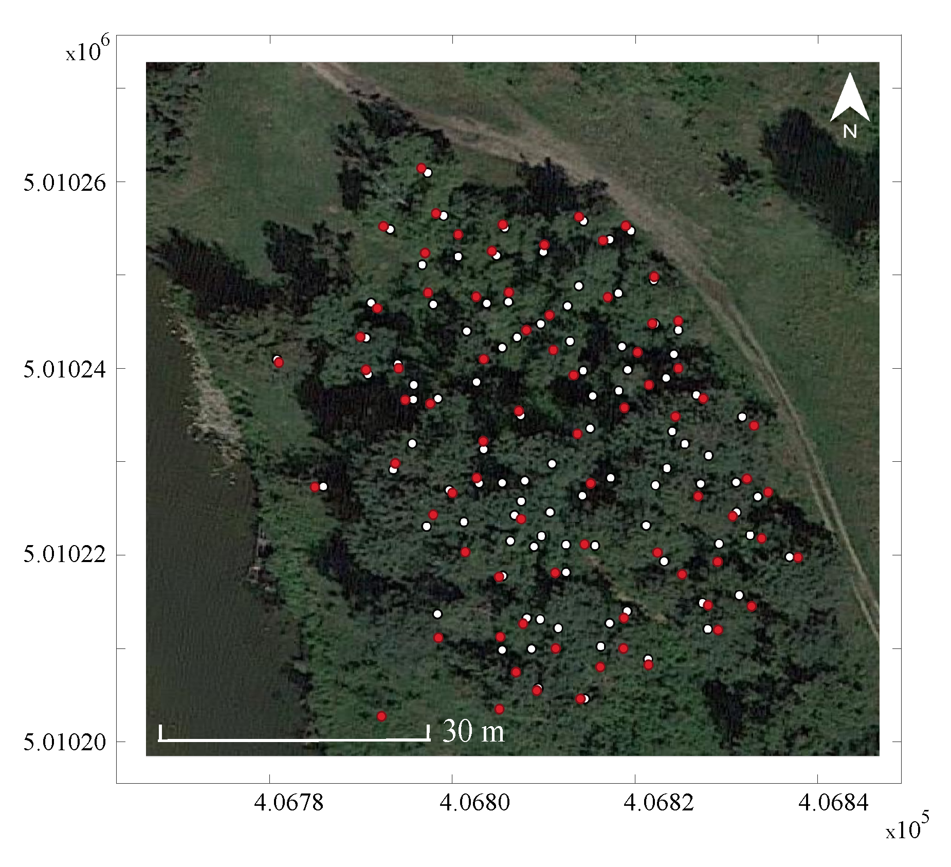
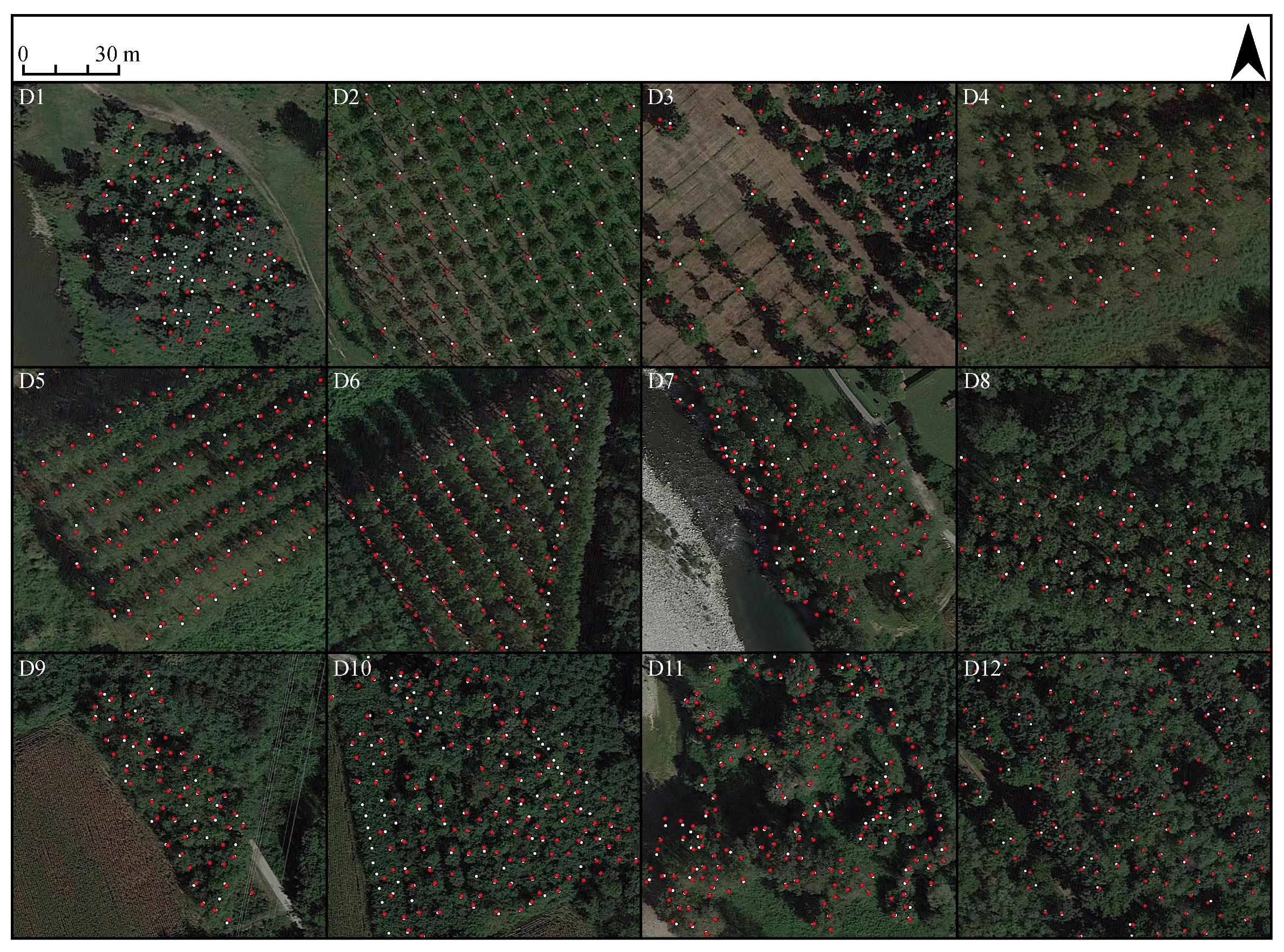
2.1. Study Site and Available Data
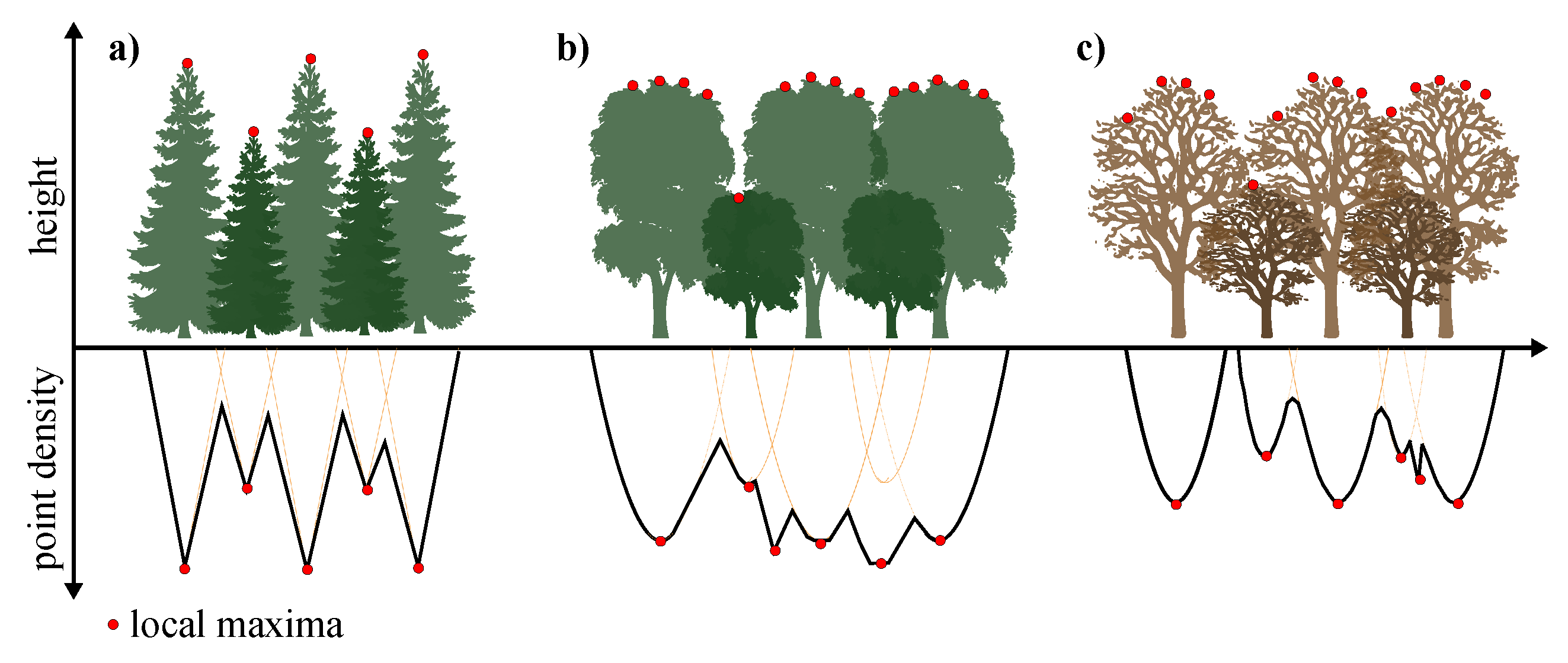
2.2. Presentation of the Algorithm
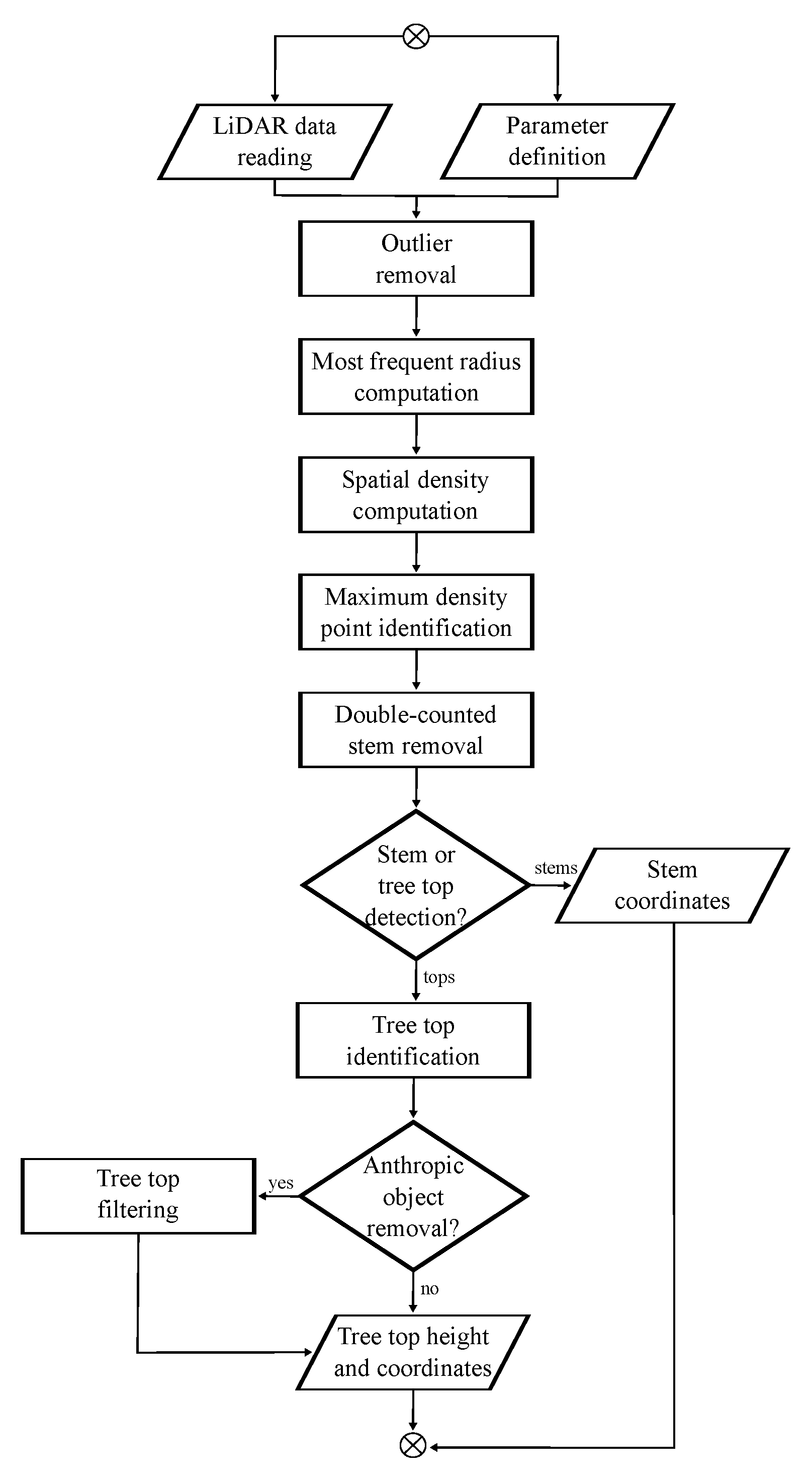
2.2.1. Pre-Processing
2.2.2. Workflow
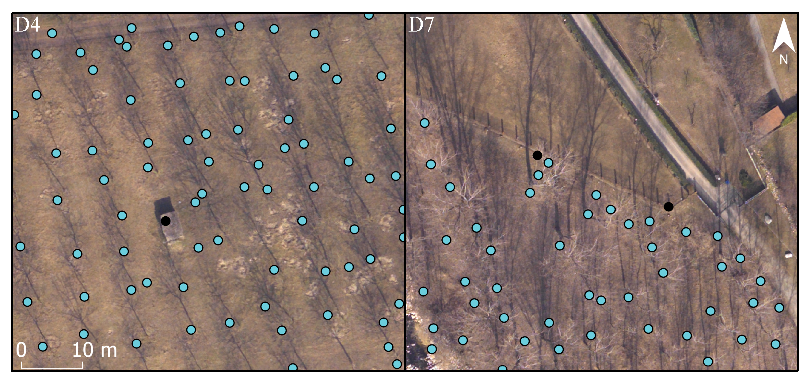
2.3. Accuracy Assessment
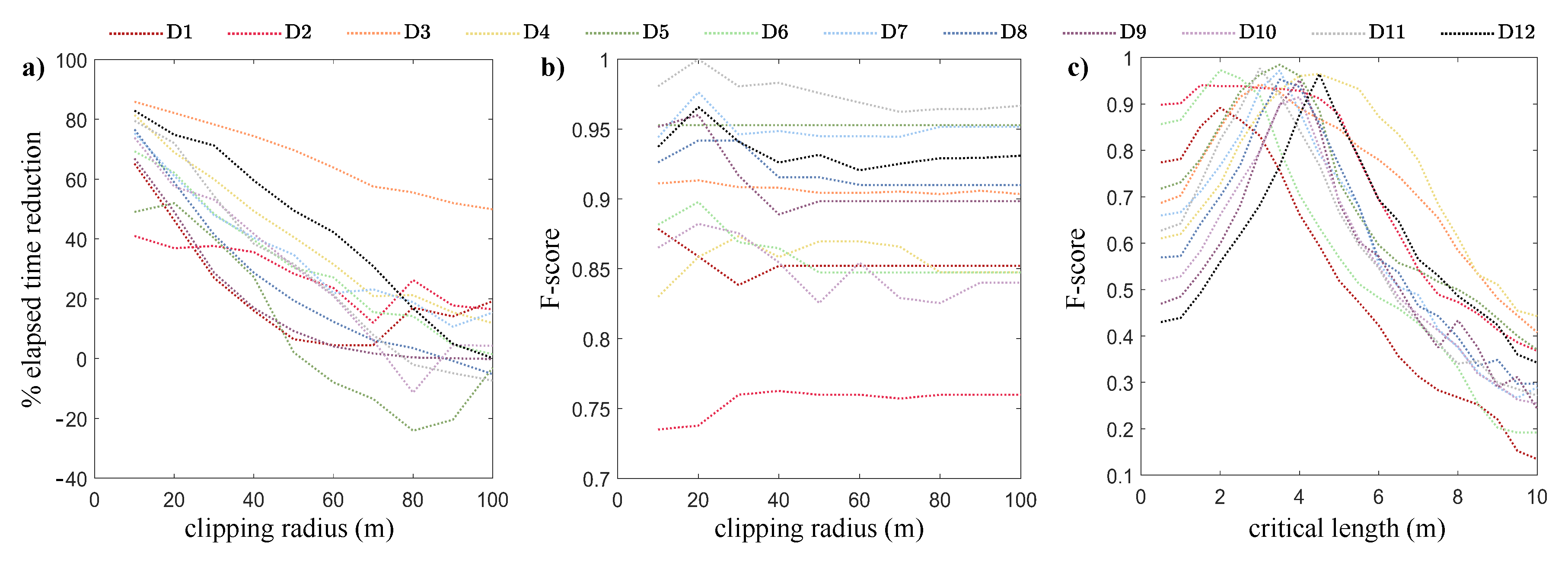
2.4. Sensitivity Analysis and the Parameter Setting
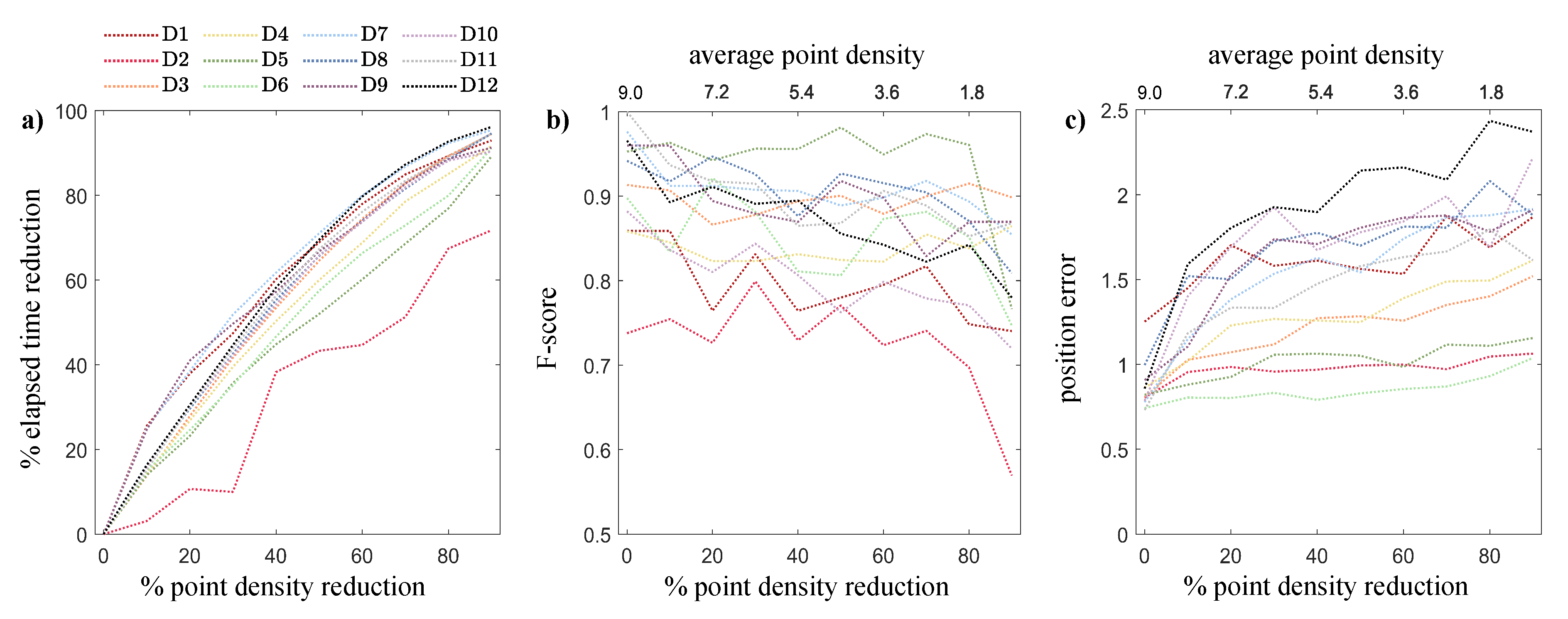
2.5. Application to Re-Sampled Point Clouds
3. Results
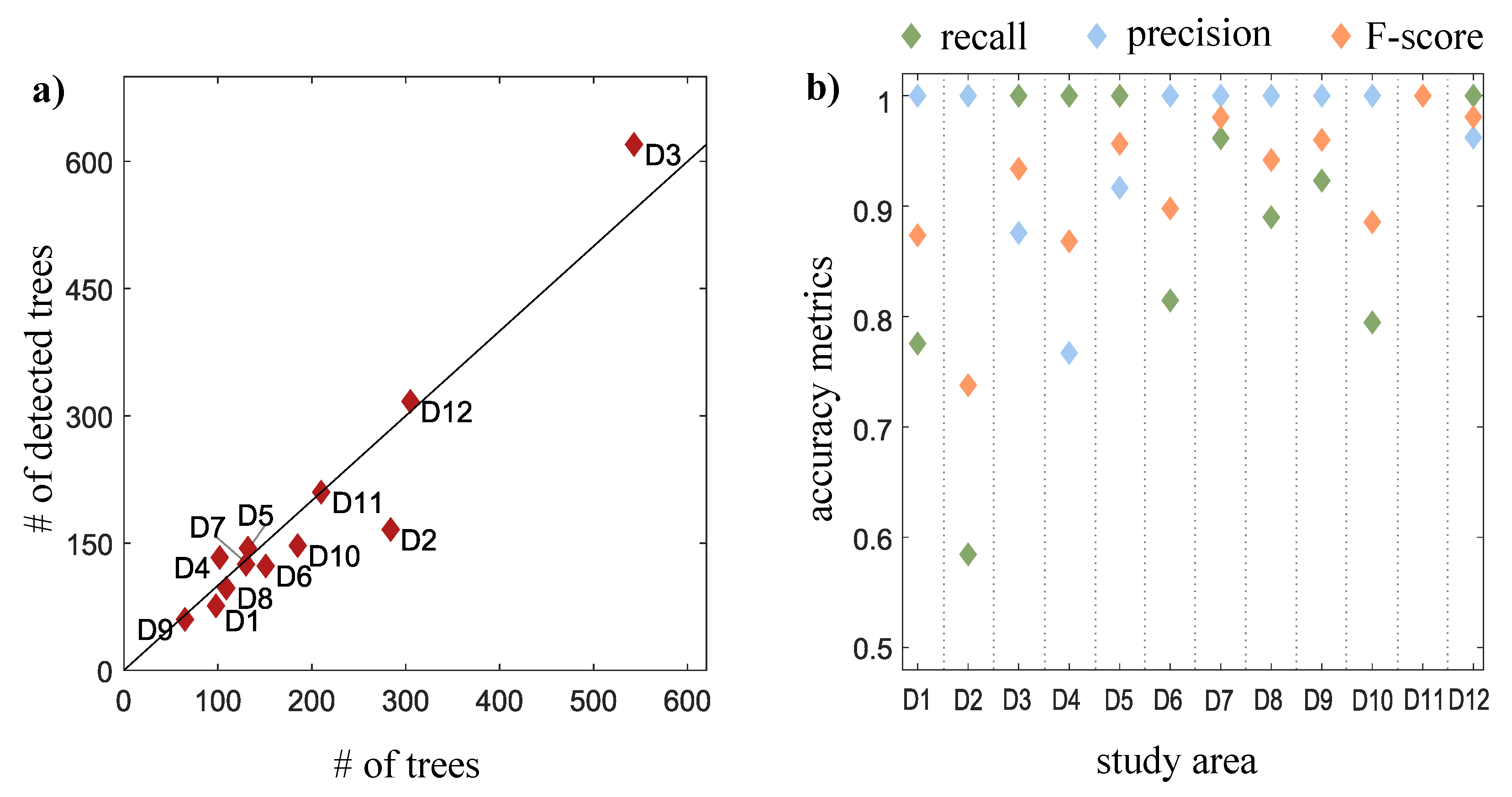
3.1. Algorithm Performance
3.2. Sensitivity Analysis Results
3.3. Re-Sampling Results
4. Discussion
4.1. Data for the Algorithm’s Application
4.2. Achieved Accuracy and the Influence of Data Quality
4.3. The Influence of the Parameter Setting
4.4. Cloud Re-Sampling and Low-Resolution Data
5. Conclusions
Supplementary Materials
Author Contributions
Funding
Institutional Review Board Statement
Informed Consent Statement
Data Availability Statement
Acknowledgments
Conflicts of Interest
Abbreviations
| ALS | Airborne Laser Scanning |
| CHM | Canopy Height Model |
| GIS | Geographic Information System |
| GPS | Global Positioning System |
| LiDAR | Light Detection And Ranging |
| RTK | Real Time Kinematic |
| TLS | Terrestrial Laser Scanning |
Appendix A. Algorithm Setup

References
- Flood, M. Laser altimetry: From science to commerical lidar mapping. Photogramm. Eng. Remote Sens. 2001, 67, 1209–1211, 1213–1217. [Google Scholar]
- Lindberg, E.; Holmgren, J. Individual tree crown methods for 3D data from remote sensing. Curr. For. Rep. 2017, 3, 19–31. [Google Scholar] [CrossRef]
- Andújar, D.; Escolà, A.; Rosell-Polo, J.R.; Fernández-Quintanilla, C.; Dorado, J. Potential of a terrestrial LiDAR-based system to characterise weed vegetation in maize crops. Comput. Electron. Agric. 2013, 92, 11–15. [Google Scholar] [CrossRef]
- Eitel, J.U.; Magney, T.S.; Vierling, L.A.; Brown, T.T.; Huggins, D.R. LiDAR based biomass and crop nitrogen estimates for rapid, non-destructive assessment of wheat nitrogen status. Field Crops Res. 2014, 159, 21–32. [Google Scholar] [CrossRef]
- Reutebuch, S.E.; McGaughey, R.J.; Andersen, H.E.; Carson, W.W. Accuracy of a high-resolution lidar terrain model under a conifer forest canopy. Can. J. Remote Sens. 2003, 29, 527–535. [Google Scholar] [CrossRef]
- Klemas, V. Beach profiling and LIDAR bathymetry: An overview with case studies. J. Coast. Res. 2011, 27, 1019–1028. [Google Scholar] [CrossRef]
- Vastaranta, M.; Kantola, T.; Lyytikäinen-Saarenmaa, P.; Holopainen, M.; Kankare, V.; Wulder, M.A.; Hyyppä, J.; Hyyppä, H. Area-based mapping of defoliation of Scots pine stands using airborne scanning LiDAR. Remote Sens. 2013, 5, 1220–1234. [Google Scholar] [CrossRef]
- Means, J.E.; Acker, S.A.; Fitt, B.J.; Renslow, M.; Emerson, L.; Hendrix, C.J. Predicting forest stand characteristics with airborne scanning lidar. Photogramm. Eng. Remote Sens. 2000, 66, 1367–1372. [Google Scholar]
- Li, Y.; Andersen, H.E.; McGaughey, R. A comparison of statistical methods for estimating forest biomass from light detection and ranging data. West. J. Appl. For. 2008, 23, 223–231. [Google Scholar] [CrossRef]
- Dalponte, M.; Reyes, F.; Kandare, K.; Gianelle, D. Delineation of individual tree crowns from ALS and hyperspectral data: A comparison among four methods. Eur. J. Remote Sens. 2015, 48, 365–382. [Google Scholar] [CrossRef]
- White, J.C.; Wulder, M.A.; Vastaranta, M.; Coops, N.C.; Pitt, D.; Woods, M. The utility of image-based point clouds for forest inventory: A comparison with airborne laser scanning. Forests 2013, 4, 518–536. [Google Scholar] [CrossRef]
- Koch, B.; Heyder, U.; Weinacker, H. Detection of individual tree crowns in airborne lidar data. Photogramm. Eng. Remote Sens. 2006, 72, 357–363. [Google Scholar] [CrossRef]
- Chen, Q. Airborne lidar data processing and information extraction. Photogramm. Eng. Remote Sens. 2007, 73, 109. [Google Scholar]
- Andersen, H.E.; Reutebuch, S.E.; Schreuder, G.F. Automated individual tree measurement through morphological analysis of a LIDAR-based canopy surface model. In Proceedings of the 1st International Precision Forestry Symposium, Seattle, WA, USA, 17–20 June 2001; pp. 11–21. [Google Scholar]
- Lee, A.C.; Lucas, R.M. A LiDAR-derived canopy density model for tree stem and crown mapping in Australian forests. Remote Sens. Environ. 2007, 111, 493–518. [Google Scholar] [CrossRef]
- Coomes, D.A.; Dalponte, M.; Jucker, T.; Asner, G.P.; Banin, L.F.; Burslem, D.F.; Lewis, S.L.; Nilus, R.; Phillips, O.L.; Phua, M.H.; et al. Area-based vs tree-centric approaches to mapping forest carbon in Southeast Asian forests from airborne laser scanning data. Remote Sens. Environ. 2017, 194, 77–88. [Google Scholar] [CrossRef]
- Yu, X.; Hyyppä, J.; Holopainen, M.; Vastaranta, M. Comparison of area-based and individual tree-based methods for predicting plot-level forest attributes. Remote Sens. 2010, 2, 1481–1495. [Google Scholar] [CrossRef]
- González-Ferreiro, E.; Diéguez-Aranda, U.; Barreiro-Fernández, L.; Buján, S.; Barbosa, M.; Suárez, J.C.; Bye, I.J.; Miranda, D. A mixed pixel-and region-based approach for using airborne laser scanning data for individual tree crown delineation in Pinus radiata D. Don plantations. Int. J. Remote Sens. 2013, 34, 7671–7690. [Google Scholar] [CrossRef]
- Corona, P.; Fattorini, L. Area-based lidar-assisted estimation of forest standing volume. Can. J. For. Res. 2008, 38, 2911–2916. [Google Scholar] [CrossRef]
- Magnussen, S.; Næsset, E.; Gobakken, T.; Frazer, G. A fine-scale model for area-based predictions of tree-size-related attributes derived from LiDAR canopy heights. Scand. J. For. Res. 2012, 27, 312–322. [Google Scholar] [CrossRef]
- Duncanson, L.; Dubayah, R. Monitoring individual tree-based change with airborne lidar. Ecol. Evol. 2018, 8, 5079–5089. [Google Scholar] [CrossRef]
- Rönnholm, P.; Hyyppä, J.; Hyyppä, H.; Haggrén, H.; Yu, X.; Kaartinen, H. Calibration of laser-derived tree height estimates by means of photogrammetric techniques. Scand. J. For. Res. 2004, 19, 524–528. [Google Scholar] [CrossRef]
- White, J.C.; Wulder, M.A.; Varhola, A.; Vastaranta, M.; Coops, N.C.; Cook, B.D.; Pitt, D.; Woods, M. A best practices guide for generating forest inventory attributes from airborne laser scanning data using an area-based approach. For. Chron. 2013, 89, 722–723. [Google Scholar] [CrossRef]
- Kandare, K.; Ørka, H.O.; Chan, J.C.W.; Dalponte, M. Effects of forest structure and airborne laser scanning point cloud density on 3D delineation of individual tree crowns. Eur. J. Remote Sens. 2016, 49, 337–359. [Google Scholar] [CrossRef]
- Hyyppä, J.; Kelle, O.; Lehikoinen, M.; Inkinen, M. A segmentation-based method to retrieve stem volume estimates from 3-D tree height models produced by laser scanners. IEEE Trans. Geosci. Remote Sens. 2001, 39, 969–975. [Google Scholar] [CrossRef]
- Persson, A.; Holmgren, J.; Soderman, U. Detecting and measuring individual trees using an airborne laser scanner. Photogramm. Eng. Remote Sens. 2002, 68, 925–932. [Google Scholar]
- Brandtberg, T.; Warner, T.A.; Landenberger, R.E.; McGraw, J.B. Detection and analysis of individual leaf-off tree crowns in small footprint, high sampling density lidar data from the eastern deciduous forest in North America. Remote Sens. Environ. 2003, 85, 290–303. [Google Scholar] [CrossRef]
- Popescu, S.C.; Wynne, R.H. Seeing the trees in the forest. Photogramm. Eng. Remote Sens. 2004, 70, 589–604. [Google Scholar] [CrossRef]
- Heurich, M.; Weinacker, H. Automated tree detection and measurement in temperate forests of central Europe using laser scanning data. Int. Arch. Photogramm. Remote Sens. Spat. Inf. Sci. 2004, 36, 8. [Google Scholar]
- Pitkänen, J.; Maltamo, M.; Hyyppä, J.; Yu, X. Adaptive methods for individual tree detection on airborne laser based canopy height model. Int. Arch. Photogramm. Remote Sens. Spat. Inf. Sci. 2004, 36, 187–191. [Google Scholar]
- Weinacker, H.; Koch, B.; Heyder, U.; Weinacker, R. Development of filtering, segmentation and modeling modules for lidar and multispectral data as a fundament of an automatic forest inventory system. Int. Arch. Photogramm. Remote Sens. Spat. Inf. Sci. 2004, 36, W2. [Google Scholar]
- Chen, Q.; Baldocchi, D.; Gong, P.; Kelly, M. Isolating individual trees in a savanna woodland using small footprint lidar data. Photogramm. Eng. Remote Sens. 2006, 72, 923–932. [Google Scholar] [CrossRef]
- Solberg, S.; Naesset, E.; Bollandsas, O.M. Single tree segmentation using airborne laser scanner data in a structurally heterogeneous spruce forest. Photogramm. Eng. Remote Sens. 2006, 72, 1369–1378. [Google Scholar] [CrossRef]
- Pang, Y.; Lefsky, M.; Andersen, H.E.; Miller, M.; Sherrill, K. Validation of the ICEsat vegetation product using crown-area-weighted mean height derived using crown delineation with discrete return lidar data. Can. J. Remote Sens. 2008, 34, S471–S484. [Google Scholar] [CrossRef]
- Maltamo, M.; Peuhkurinen, J.; Malinen, J.; Vauhkonen, J.; Packalén, P.; Tokola, T. Predicting tree attributes and quality characteristics of Scots pine using airborne laser scanning data. Silva Fenn. 2009, 43, 507–521. [Google Scholar] [CrossRef]
- Yu, X.; Hyyppä, J.; Vastaranta, M.; Holopainen, M.; Viitala, R. Predicting individual tree attributes from airborne laser point clouds based on the random forests technique. ISPRS J. Photogramm. Remote Sens. 2011, 66, 28–37. [Google Scholar] [CrossRef]
- Ene, L.; Næsset, E.; Gobakken, T. Single tree detection in heterogeneous boreal forests using airborne laser scanning and area-based stem number estimates. Int. J. Remote Sens. 2012, 33, 5171–5193. [Google Scholar] [CrossRef]
- Jing, L.; Hu, B.; Li, J.; Noland, T. Automated delineation of individual tree crowns from LiDAR data by multi-scale analysis and segmentation. Photogramm. Eng. Remote Sens. 2012, 78, 1275–1284. [Google Scholar] [CrossRef]
- Dalponte, M.; Coomes, D.A. Tree-centric mapping of forest carbon density from airborne laser scanning and hyperspectral data. Methods Ecol. Evol. 2016, 7, 1236–1245. [Google Scholar] [CrossRef]
- Silva, C.A.; Hudak, A.T.; Vierling, L.A.; Loudermilk, E.L.; O’Brien, J.J.; Hiers, J.K.; Jack, S.B.; Gonzalez-Benecke, C.; Lee, H.; Falkowski, M.J.; et al. Imputation of individual longleaf pine (Pinus palustris Mill.) tree attributes from field and LiDAR data. Can. J. Remote Sens. 2016, 42, 554–573. [Google Scholar] [CrossRef]
- Bian, Y.; Zou, P.; Shu, Y.; Yu, R. Individual tree delineation in deciduous forest areas with LiDAR point clouds. Can. J. Remote Sens. 2014, 40, 152–163. [Google Scholar] [CrossRef]
- Hirata, Y.; Furuya, N.; Suzuki, M.; Yamamoto, H. Airborne laser scanning in forest management: Individual tree identification and laser pulse penetration in a stand with different levels of thinning. For. Ecol. Manag. 2009, 258, 752–760. [Google Scholar] [CrossRef]
- Duncanson, L.; Cook, B.; Hurtt, G.; Dubayah, R. An efficient, multi-layered crown delineation algorithm for mapping individual tree structure across multiple ecosystems. Remote Sens. Environ. 2014, 154, 378–386. [Google Scholar] [CrossRef]
- Zhao, D.; Pang, Y.; Li, Z.; Liu, L. Isolating individual trees in a closed coniferous forest using small footprint lidar data. Int. J. Remote Sens. 2014, 35, 7199–7218. [Google Scholar] [CrossRef]
- Kwak, D.A.; Lee, W.K.; Lee, J.H.; Biging, G.S.; Gong, P. Detection of individual trees and estimation of tree height using LiDAR data. J. For. Res. 2007, 12, 425–434. [Google Scholar] [CrossRef]
- Leckie, D.; Gougeon, F.; Hill, D.; Quinn, R.; Armstrong, L.; Shreenan, R. Combined high-density lidar and multispectral imagery for individual tree crown analysis. Can. J. Remote Sens. 2003, 29, 633–649. [Google Scholar] [CrossRef]
- Falkowski, M.J.; Smith, A.M.; Hudak, A.T.; Gessler, P.E.; Vierling, L.A.; Crookston, N.L. Automated estimation of individual conifer tree height and crown diameter via two-dimensional spatial wavelet analysis of lidar data. Can. J. Remote Sens. 2006, 32, 153–161. [Google Scholar] [CrossRef]
- Wu, B.; Yu, B.; Wu, Q.; Huang, Y.; Chen, Z.; Wu, J. Individual tree crown delineation using localized contour tree method and airborne LiDAR data in coniferous forests. Int. J. Appl. Earth Obs. Geoinf. 2016, 52, 82–94. [Google Scholar] [CrossRef]
- Rahman, M.; Gorte, B. Tree crown delineation from high resolution airborne lidar based on densities of high points. In Proceedings of the ISPRS Workshop Laserscanning 2009, ISPRS XXXVIII (3/W8), Paris, France, 1–2 September 2009. [Google Scholar]
- Richardson, J.J.; Moskal, L.M. Strengths and limitations of assessing forest density and spatial configuration with aerial LiDAR. Remote Sens. Environ. 2011, 115, 2640–2651. [Google Scholar] [CrossRef]
- Li, W.; Guo, Q.; Jakubowski, M.K.; Kelly, M. A new method for segmenting individual trees from the lidar point cloud. Photogramm. Eng. Remote Sens. 2012, 78, 75–84. [Google Scholar] [CrossRef]
- Hu, B.; Li, J.; Jing, L.; Judah, A. Improving the efficiency and accuracy of individual tree crown delineation from high-density LiDAR data. Int. J. Appl. Earth Obs. Geoinf. 2014, 26, 145–155. [Google Scholar] [CrossRef]
- Mongus, D.; Žalik, B. An efficient approach to 3D single tree-crown delineation in LiDAR data. ISPRS J. Photogramm. Remote Sens. 2015, 108, 219–233. [Google Scholar] [CrossRef]
- Reitberger, J.; Schnörr, C.; Krzystek, P.; Stilla, U. 3D segmentation of single trees exploiting full waveform LIDAR data. ISPRS J. Photogramm. Remote Sens. 2009, 64, 561–574. [Google Scholar] [CrossRef]
- Holmgren, J.; Lindberg, E. Tree crown segmentation based on a geometric tree crown model for prediction of forest variables. Can. J. Remote Sens. 2013, 39, S86–S98. [Google Scholar] [CrossRef]
- Holmgren, J.; Lindberg, E. Tree crown segmentation based on a tree crown density model derived from Airborne Laser Scanning. Remote Sens. Lett. 2019, 10, 1143–1152. [Google Scholar] [CrossRef]
- Lu, X.; Guo, Q.; Li, W.; Flanagan, J. A bottom-up approach to segment individual deciduous trees using leaf-off lidar point cloud data. ISPRS J. Photogramm. Remote Sens. 2014, 94, 1–12. [Google Scholar] [CrossRef]
- Morsdorf, F.; Meier, E.; Kötz, B.; Itten, K.I.; Dobbertin, M.; Allgöwer, B. LIDAR-based geometric reconstruction of boreal type forest stands at single tree level for forest and wildland fire management. Remote Sens. Environ. 2004, 92, 353–362. [Google Scholar] [CrossRef]
- Tiede, D.; Hochleitner, G.; Blaschke, T. A full GIS-based workflow for tree identification and tree crown delineation using laser scanning. In Proceedings of the ISPRS Workshop CMRT, Vienna, Austria, 29–30 August 2005; Volume 5. [Google Scholar]
- Lee, H.; Slatton, K.C.; Roth, B.E.; Cropper, W., Jr. Adaptive clustering of airborne LiDAR data to segment individual tree crowns in managed pine forests. Int. J. Remote Sens. 2010, 31, 117–139. [Google Scholar] [CrossRef]
- Véga, C.; Hamrouni, A.; El Mokhtari, S.; Morel, J.; Bock, J.; Renaud, J.P.; Bouvier, M.; Durrieu, S. PTrees: A point-based approach to forest tree extraction from lidar data. Int. J. Appl. Earth Obs. Geoinf. 2014, 33, 98–108. [Google Scholar] [CrossRef]
- Ayrey, E.; Fraver, S.; Kershaw, J.A., Jr.; Kenefic, L.S.; Hayes, D.; Weiskittel, A.R.; Roth, B.E. Layer stacking: A novel algorithm for individual forest tree segmentation from LiDAR point clouds. Can. J. Remote Sens. 2017, 43, 16–27. [Google Scholar] [CrossRef]
- Ma, Z.; Pang, Y.; Wang, D.; Liang, X.; Chen, B.; Lu, H.; Weinacker, H.; Koch, B. Individual Tree Crown Segmentation of a Larch Plantation Using Airborne Laser Scanning Data Based on Region Growing and Canopy Morphology Features. Remote Sens. 2020, 12, 1078. [Google Scholar] [CrossRef]
- Rahman, M.; Gorte, B. Individual tree detection based on densities of high points of high resolution airborne LiDAR. In Proceedings of the GEOBIA, 2008—Pixels, Objects, Intelligence: GEOgraphic Object Based Image Analysis for the 21st Century, Calgary, AB, Canada, 5–8 August 2008; University of Calgary: Calgary, AB, Canada, 2008; pp. 350–355. [Google Scholar]
- Rahman, M.; Gorte, B. Tree filtering for high density airborne LiDAR data. In Proceedings of the International Conference on LiDAR Applications in Forest Assessment and Inventory, Edinburgh, UK, 17–19 September 2008. [Google Scholar]
- Ferraz, A.; Bretar, F.; Jacquemoud, S.; Gonçalves, G.; Pereira, L.; Tomé, M.; Soares, P. 3-D mapping of a multi-layered Mediterranean forest using ALS data. Remote Sens. Environ. 2012, 121, 210–223. [Google Scholar] [CrossRef]
- Paris, C.; Valduga, D.; Bruzzone, L. A hierarchical approach to three-dimensional segmentation of LiDAR data at single-tree level in a multilayered forest. IEEE Trans. Geosci. Remote Sens. 2016, 54, 4190–4203. [Google Scholar] [CrossRef]
- Zhen, Z.; Quackenbush, L.J.; Zhang, L. Trends in automatic individual tree crown detection and delineation—Evolution of LiDAR data. Remote Sens. 2016, 8, 333. [Google Scholar] [CrossRef]
- Dai, W.; Yang, B.; Dong, Z.; Shaker, A. A new method for 3D individual tree extraction using multispectral airborne LiDAR point clouds. ISPRS J. Photogramm. Remote Sens. 2018, 144, 400–411. [Google Scholar] [CrossRef]
- Gupta, S.; Weinacker, H.; Koch, B. Comparative analysis of clustering-based approaches for 3-D single tree detection using airborne fullwave lidar data. Remote Sens. 2010, 2, 968–989. [Google Scholar] [CrossRef]
- Yao, W.; Krzystek, P.; Heurich, M. Tree species classification and estimation of stem volume and DBH based on single tree extraction by exploiting airborne full-waveform LiDAR data. Remote Sens. Environ. 2012, 123, 368–380. [Google Scholar] [CrossRef]
- Liang, X.; Litkey, P.; Hyyppä, J.; Kaartinen, H.; Kukko, A.; Holopainen, M. Automatic plot-wise tree location mapping using single-scan terrestrial laser scanning. Photogramm. J. Finl. 2011, 22, 37–48. [Google Scholar]
- Olofsson, K.; Holmgren, J.; Olsson, H. Tree stem and height measurements using terrestrial laser scanning and the RANSAC algorithm. Remote Sens. 2014, 6, 4323–4344. [Google Scholar] [CrossRef]
- Trochta, J.; Krůček, M.; Vrška, T.; Král, K. 3D Forest: An application for descriptions of three-dimensional forest structures using terrestrial LiDAR. PLoS ONE 2017, 12, e0176871. [Google Scholar] [CrossRef]
- Kuželka, K.; Slavík, M.; Surovỳ, P. Very High Density Point Clouds from UAV Laser Scanning for Automatic Tree Stem Detection and Direct Diameter Measurement. Remote Sens. 2020, 12, 1236. [Google Scholar] [CrossRef]
- Roussel, J.R.; Caspersen, J.; Béland, M.; Thomas, S.; Achim, A. Removing bias from LiDAR-based estimates of canopy height: Accounting for the effects of pulse density and footprint size. Remote Sens. Environ. 2017, 198, 1–16. [Google Scholar] [CrossRef]
- Goutte, C.; Gaussier, E. A probabilistic interpretation of precision, recall and F-score, with implication for evaluation. In Proceedings of the European Conference on Information Retrieval, Santiago de Compostela, Spain, 21–23 March 2005; Springer: Berlin/Heidelberg, Germany, 2005; pp. 345–359. [Google Scholar]
- Bechtold, W.A. Crown-diameter prediction models for 87 species of stand-grown trees in the eastern United States. South. J. Appl. For. 2003, 27, 269–278. [Google Scholar] [CrossRef]
- Pretzsch, H.; Biber, P.; Uhl, E.; Dahlhausen, J.; Rötzer, T.; Caldentey, J.; Koike, T.; Van Con, T.; Chavanne, A.; Seifert, T.; et al. Crown size and growing space requirement of common tree species in urban centers, parks, and forests. Urban For. Urban Green. 2015, 14, 466–479. [Google Scholar] [CrossRef]
- Graham, A.N.; Coops, N.C.; Tompalski, P.; Plowright, A.; Wilcox, M. Effect of ground surface interpolation methods on the accuracy of forest attribute modeling using unmanned aerial systems-based digital aerial photogrammetry. Int. J. Remote Sens. 2020, 41, 3287–3306. [Google Scholar] [CrossRef]
- Habib, M.; Alzubi, Y.; Malkawi, A.; Awwad, M. Impact of interpolation techniques on the accuracy of large-scale digital elevation model. Open Geosci. 2020, 12, 190–202. [Google Scholar] [CrossRef]
- Liu, Q.; Fu, L.; Chen, Q.; Wang, G.; Luo, P.; Sharma, R.P.; He, P.; Li, M.; Wang, M.; Duan, G. Analysis of the Spatial Differences in Canopy Height Models from UAV LiDAR and Photogrammetry. Remote Sens. 2020, 12, 2884. [Google Scholar] [CrossRef]
- Lovell, J.; Jupp, D.; Newnham, G.; Coops, N.; Culvenor, D. Simulation study for finding optimal lidar acquisition parameters for forest height retrieval. For. Ecol. Manag. 2005, 214, 398–412. [Google Scholar] [CrossRef]
- Holmgren, J.; Nilsson, M.; Olsson, H. Simulating the effects of lidar scanning angle for estimation of mean tree height and canopy closure. Can. J. Remote Sens. 2003, 29, 623–632. [Google Scholar] [CrossRef]
- Gaulton, R.; Malthus, T.J. LiDAR mapping of canopy gaps in continuous cover forests: A comparison of canopy height model and point cloud based techniques. Int. J. Remote Sens. 2010, 31, 1193–1211. [Google Scholar] [CrossRef]
- Disney, M.I.; Kalogirou, V.; Lewis, P.; Prieto-Blanco, A.; Hancock, S.; Pfeifer, M. Simulating the impact of discrete-return lidar system and survey characteristics over young conifer and broadleaf forests. Remote Sens. Environ. 2010, 114, 1546–1560. [Google Scholar] [CrossRef]
- Keränen, J.; Maltamo, M.; Packalen, P. Effect of flying altitude, scanning angle and scanning mode on the accuracy of ALS based forest inventory. Int. J. Appl. Earth Obs. Geoinf. 2016, 52, 349–360. [Google Scholar] [CrossRef]
- Liu, J.; Skidmore, A.K.; Jones, S.; Wang, T.; Heurich, M.; Zhu, X.; Shi, Y. Large off-nadir scan angle of airborne LiDAR can severely affect the estimates of forest structure metrics. ISPRS J. Photogramm. Remote Sens. 2018, 136, 13–25. [Google Scholar] [CrossRef]
- Mielcarek, M.; Stereńczak, K.; Khosravipour, A. Testing and evaluating different LiDAR-derived canopy height model generation methods for tree height estimation. Int. J. Appl. Earth Obs. Geoinf. 2018, 71, 132–143. [Google Scholar] [CrossRef]
- García, M.; Riaño, D.; Chuvieco, E.; Danson, F.M. Estimating biomass carbon stocks for a Mediterranean forest in central Spain using LiDAR height and intensity data. Remote Sens. Environ. 2010, 114, 816–830. [Google Scholar] [CrossRef]
- Mitchell, B.; Walterman, M.; Mellin, T.; Wilcox, C.; Lynch, A.M.; Anhold, J.; Falk, D.A.; Koprowski, J.; Laes, D.; Evans, D.; et al. Mapping vegetation structure in the Pinaleño Mountains using lidar-phase 3: Forest inventory modeling. In RSAC-100007-RPT1; US Department of Agriculture, Forest Service, Remote Sensing Applications Center: Salt Lake City, UT, USA, 2012; 17p. [Google Scholar]
- Lefsky, M.A.; Cohen, W.B.; Parker, G.G.; Harding, D.J. Lidar remote sensing for ecosystem studies. BioScience 2002, 52, 19–30. [Google Scholar] [CrossRef]
- Gaveau, D.L.; Hill, R.A. Quantifying canopy height underestimation by laser pulse penetration in small-footprint airborne laser scanning data. Can. J. Remote Sens. 2003, 29, 650–657. [Google Scholar] [CrossRef]
- Meng, X.; Currit, N.; Zhao, K. Ground filtering algorithms for airborne LiDAR data: A review of critical issues. Remote Sens. 2010, 2, 833–860. [Google Scholar] [CrossRef]
- Parkan, M. Digital Forestry Toolbox for Matlab/Octave. Zenodo. 2018. Available online: https://zenodo.org/badge/latestdoi/58712667 (accessed on 27 August 2020).
- White, J.C.; Coops, N.C.; Wulder, M.A.; Vastaranta, M.; Hilker, T.; Tompalski, P. Remote sensing technologies for enhancing forest inventories: A review. Can. J. Remote Sens. 2016, 42, 619–641. [Google Scholar] [CrossRef]
- Camporeale, C.; Ridolfi, L. Noise-induced phenomena in riparian vegetation dynamics. Geophys. Res. Lett. 2007, 34. [Google Scholar] [CrossRef]
- Vesipa, R.; Camporeale, C.; Ridolfi, L. Noise-driven cooperative dynamics between vegetation and topography in riparian zones. Geophys. Res. Lett. 2015, 42, 8021–8030. [Google Scholar] [CrossRef]
- Latella, M.; Bertagni, M.B.; Vezza, P.; Camporeale, C. An integrated methodology to study riparian vegetation dynamics: From field data to impact modeling. J. Adv. Model. Earth Syst. 2020, 12, e2020MS002094. [Google Scholar] [CrossRef] [PubMed]


| Area ID | Coordinates | Tree | Tree | Tree | Perimeter | Area | Point | Notes |
|---|---|---|---|---|---|---|---|---|
| Pattern | Species | Age | (m) | (ha) | Density | |||
| D1 | 451422.27N; | random | Populus spp., | mature | 240 | 0.41 | 8.7 ± 4.4 | - |
| 074845.10E | Robinia Ps. | |||||||
| D2 | 451901.73N; | regular | Populus spp. | various | 620 | 2.40 | 7.5 ± 4.2 | - |
| 074416.98E | ||||||||
| D3 | 451206.02N; | mixed | Populus spp. | young | 834 | 4.39 | 8.7 ± 3.7 | - |
| 075026.61E | ||||||||
| D4 | 451058.61N; | regular | Populus spp. | various | 332 | 0.68 | 5.8 ± 2.1 | a warehouse |
| 075207.15E | 4 × 4 ×2 m | |||||||
| D5 | 451144.09N; | regular | Populus spp. | mature | 313 | 0.40 | 10.2 ± 3.4 | - |
| 075136.33E | ||||||||
| D6 | 451140.61N; | regular | Populus spp. | mature | 308 | 0.57 | 9.6 ± 3.6 | - |
| 075138.04E | ||||||||
| D7 | 452002.58N; | random | Populus spp. | various | 339 | 0.62 | 13.5 ± 7.5 | fence |
| 074401.05E | height: 2.5 m | |||||||
| D8 | 451225.45N; | regular | Populus spp., | mature | 316 | 0.41 | 17.8 ± 8.1 | - |
| 075032.02E | Quercus spp. | |||||||
| D9 | 451806.05N; | random | Robinia Ps. | mature | 250 | 0.27 | 10.1 ± 5.4 | power lines |
| 074603.51E | ||||||||
| D10 | 451808.24N; | mixed | Populus spp., | mature | 357 | 0.81 | 8.2 ± 4.6 | - |
| 074559.95E | Robinia Ps. | |||||||
| D11 | 451234.08N | random | Populus spp., | mature | 435 | 1.20 | 11.9 ± 7.2 | - |
| 075006.51E | Quercus spp. | |||||||
| D12 | 451206.08N; | regular | Populus spp. | mature | 572 | 1.93 | 8.7 ± 3.8 | - |
| 075026.58E |
| Area ID | # of Trees | # of Detected Trees | Recall | Precision | F-Score | Position Error (m) | Stem-to-Top Distance (m) | ||
|---|---|---|---|---|---|---|---|---|---|
| Min | Max | Mean | |||||||
| D1 | 98 | 76 | 0.78 | 0.96 | 0.86 | 1.25 | 0 | 2.12 | 0.79 |
| D2 | 284 | 166 | 0.58 | 1.00 | 0.74 | 0.80 | 0 | 2.08 | 0.63 |
| D3 | 543 | 620 | 1.00 | 0.84 | 0.92 | 0.81 | 0 | 2.06 | 0.62 |
| D4 | 102 | 133 | 1.00 | 0.75 | 0.86 | 0.86 | 0 | 1.67 | 0.65 |
| D5 | 132 | 144 | 1.00 | 0.91 | 0.95 | 0.82 | 0 | 1.79 | 0.53 |
| D6 | 151 | 123 | 0.81 | 1.00 | 0.90 | 0.74 | 0 | 1.35 | 0.54 |
| D7 | 130 | 125 | 0.96 | 0.99 | 0.98 | 0.78 | 0 | 1.70 | 0.66 |
| D8 | 109 | 97 | 0.89 | 1.00 | 0.94 | 1.00 | 0 | 1.31 | 0.60 |
| D9 | 65 | 60 | 0.92 | 1.00 | 0.96 | 0.91 | 0 | 1.19 | 0.56 |
| D10 | 185 | 147 | 0.79 | 0.99 | 0.78 | 0.91 | 0 | 1.91 | 0.55 |
| D11 | 210 | 210 | 1.00 | 1.00 | 1.00 | 0.73 | 0 | 1.50 | 0.63 |
| D12 | 305 | 317 | 1.00 | 0.93 | 0.97 | 0.86 | 0 | 1.83 | 0.70 |
| Area ID | Elapsed Time (s) | Number of Points |
|---|---|---|
| D1 | 41.87 | 19,510 |
| D2 | 4.28 | 4500 |
| D3 | 195.09 | 97,568 |
| D4 | 36.55 | 24,679 |
| D5 | 11.42 | 9995 |
| D6 | 17.43 | 13,391 |
| D7 | 142.93 | 45,617 |
| D8 | 59.91 | 29,935 |
| D9 | 34.75 | 15,860 |
| D10 | 55.00 | 31,865 |
| D11 | 123.91 | 58,808 |
| D12 | 413.62 | 127,192 |
| Area ID | Real Spacing (m) | Optimal Spacing (m) | Computed Spacing (m) |
|---|---|---|---|
| D1 | 2.5 | 2.0 | 2.8 |
| D2 | 6.0 | 1.5 | 5.8 |
| D3 | 3.0 | 3.0 | 2.5 |
| D4 | 8.0 | 4.0 | 2.8 |
| D5 | 5.0 | 3.5 | 2.8 |
| D6 | 2.5 | 2.0 | 3.1 |
| D7 | 3.5 | 3.5 | 3.3 |
| D8 | 3.5 | 3.5 | 3.8 |
| D9 | 4.0 | 4.0 | 4.1 |
| D10 | 4.0 | 4.0 | 4.2 |
| D11 | 3.0 | 3.0 | 3.1 |
| D12 | 5.0 | 4.5 | 4.4 |
| Advantages | Limitations | Notes |
|---|---|---|
| Low sensitivity to the tree spatial arrangement and the presence of understory vegetation. | Better performance in homogenous stands. | Splitting of datasets into homogenous areas before its application. |
| Working on the entire point clouds. | Long computation time for high number of input points. | In the case of large datasets, algorithm’s parallelization or dataset’s sub-sampling. |
| Requiring 2 points·m as minimum point density | Worse performance if dealing with local data inaccuracies | Data quality inspection before its application. |
| Good accuracy with the default parameter setting. | Necessity of field calibration for the derived treetops height. | Visual inspection of the study areas before its application. |
Publisher’s Note: MDPI stays neutral with regard to jurisdictional claims in published maps and institutional affiliations. |
© 2021 by the authors. Licensee MDPI, Basel, Switzerland. This article is an open access article distributed under the terms and conditions of the Creative Commons Attribution (CC BY) license (http://creativecommons.org/licenses/by/4.0/).
Share and Cite
Latella, M.; Sola, F.; Camporeale, C. A Density-Based Algorithm for the Detection of Individual Trees from LiDAR Data. Remote Sens. 2021, 13, 322. https://doi.org/10.3390/rs13020322
Latella M, Sola F, Camporeale C. A Density-Based Algorithm for the Detection of Individual Trees from LiDAR Data. Remote Sensing. 2021; 13(2):322. https://doi.org/10.3390/rs13020322
Chicago/Turabian StyleLatella, Melissa, Fabio Sola, and Carlo Camporeale. 2021. "A Density-Based Algorithm for the Detection of Individual Trees from LiDAR Data" Remote Sensing 13, no. 2: 322. https://doi.org/10.3390/rs13020322
APA StyleLatella, M., Sola, F., & Camporeale, C. (2021). A Density-Based Algorithm for the Detection of Individual Trees from LiDAR Data. Remote Sensing, 13(2), 322. https://doi.org/10.3390/rs13020322