Article

A Density-Based Algorithm for the Detection of Individual Trees from LiDAR Data

DIATI—Department of Environmental, Land and Infrastructure Engineering, Politecnico di Torino, 10129 Torino, Italy
*
Author to whom correspondence should be addressed.
Remote Sens. 2021, 13(2), 322; https://doi.org/10.3390/rs13020322
Submission received: 3 December 2020 / Revised: 14 January 2021 / Accepted: 15 January 2021 / Published: 19 January 2021
(This article belongs to the Special Issue 3D Point Clouds in Forest Remote Sensing)

Abstract

:
Nowadays, LiDAR is widely used for individual tree detection, usually providing higher accuracy in coniferous stands than in deciduous ones, where the rounded-crown, the presence of understory vegetation, and the random spatial tree distribution may affect the identification algorithms. In this work, we propose a novel algorithm that aims to overcome these difficulties and yield the coordinates and the height of the individual trees on the basis of the point density features of the input point cloud. The algorithm was tested on twelve deciduous areas, assessing its performance on both regular-patterned plantations and stands with randomly distributed trees. For all cases, the algorithm provides high accuracy tree count (F-score > 0.7) and satisfying stem locations (position error around 1.0 m). In comparison to other common tools, the algorithm is weakly sensitive to the parameter setup and can be applied with little knowledge of the study site, thus reducing the effort and cost of field campaigns. Furthermore, it demonstrates to require just 2 points·m 2 as minimum point density, allowing for the analysis of low-density point clouds. Despite its simplicity, it may set the basis for more complex tools, such as those for crown segmentation or biomass computation, with potential applications in forest modeling and management.

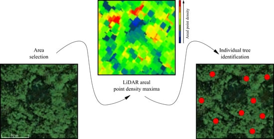
Graphical Abstract

1. Introduction

Light Detection and Ranging (LiDAR) is an active remote sensing system whose output consists of a three-dimensional point cloud representing the Earth’s surface and all the objects standing on it.
Starting from the 1990s, LiDAR became commercially available, thus allowing for an acceleration of its technical improvement and field applications [1,2]. Nowadays, applications involve terrestrial, airborne, and spaceborne systems and concern agriculture [3,4], geomatics [5,6], and forestry [7,8], to mention just a few. The ability of LiDAR systems to capture the complex structure of trees and forests is related to the different returns provided by the surfaces when they are intercepted by the LiDAR signal. Vegetation partially reflects and transmits the signal, so multiple returns from a single shot may occur before the last one from the ground is received. Therefore, the vertical characterization of the vegetation structures is possible [2,8,9] and LiDAR-derived data can be efficiently used to determine forest inventory parameters [10].
Thanks to its features, LiDAR is complementary to or more advantageous than other methods, such as photogrammetry and ground-based data collection, for the characterization of some forest attributes. Monoscopic photogrammetry allows for coarse-scale investigations but does not provide three-dimensional information. Stereoscopy can return a three-dimensional point cloud, but this cloud just describes the upper surface of the canopy in forested areas, thus avoiding the investigation of the under-canopy vegetation structures [11]. Ground-based methods, despite providing numerous information about individual trees and tree plots, are time-consuming, labour-intensive, expensive, and circumscribed to relatively small areas [8].
Forest inventories are fundamental for natural resources management. For instance, a record of the past and present status of forests can be generated on the basis of inventory parameters, and used to evaluate forest damage [12,13], plan environmental and commercial activities, and model future forest evolution [14]. Furthermore, data of forest inventory are essential for carbon accounting and fire-related risk assessment [15,16], and for the development of a sustainable bio-economy that grounds on renewable resources [2]. Forest information can be derived by LiDAR data according to two main approaches, namely the area-based and the individual tree-based approaches (see [16,17,18] for detailed information about the features, advantages, and disadvantages of the two approaches). The former approach generally predicts the mean features at the stand level (e.g., mean tree height diameter, basal area, volume, and biomass) from the percentiles of the LiDAR-derived height distribution [19,20]. The individual tree-based approach, instead, aims to collect specific information from which deriving other attributes, such as the biomass and the diameter-at-breast height, of each tree by means of existing models [21]. When the estimation parameters (area-based) or the LiDAR-derived metrics (individual tree-based) are calibrated on the basis of ground data, both of the methods generate accurate forest structural information that can support forest inventory over large areas [22,23].
Within the frame of individual tree-based forest inventories, the identification of trees and the assessment of their height and position play a fundamental role as they constitute the basis to derive other tree attributes [24]. Although the literature provides a large number of works dedicated to the identification of individual trees from LiDAR data, most of the proposed methodologies rely on the adoption of similar approaches, which can be roughly classified into two families, namely the canopy height models-based (CHM) and the cloud-based approaches.
Canopy Height Model (CHM)-based approaches identify the treetops by applying algorithms to the canopy height model, namely the surface model representing the top layer of canopies through its relative height with respect to the ground. This family of approaches can be further divided into classes according to their underlying algorithm: (i) the local maxima methods, which are the most frequently found in literature [12,25,26,27,28,29,30,31,32,33,34,35,36,37,38,39,40]; (ii) the local curvature methods [41]; (iii) the watershed methods, which find the tree crowns through a pouring mechanism [42,43,44]; (iv) the morphological methods, which apply opening operations to isolate the tree crowns within the CHM [13,14,45], and (v) other methods, which delineate potential crown material so that the individual trees can be distinguished [18,46,47,48]. The main difference among these classes is that the former two carry out the crown segmentation after the treetop identification, whereas the latter three perform the tree identification by looking for the treetop within the segmented crown boundaries. The CHM-based approach has proven to be quite effective in very regular vegetation pattern, especially when only one layer of the tree canopy is present, and in coniferous stands. Nevertheless, this approach may provide lower-accuracy results when applied under particular conditions [37,49,50,51,52,53]: the interpolated surfaces can be affected by the noise of the LiDAR data they derive from and by the complexity of the terrain and canopy geometry so that the tree counting process can be misleading; moreover, the presence of mixed-species forests, random tree patterns, and shade-tolerant species can affect the identification process.
As reported by Richardson and Moskal [50], some attempts have been made to overcome the aforementioned intrinsic weaknesses of the CHM-based approaches. For instance, the CHM has been used together with full-waveform LiDAR datasets [54], combined to a new inventory index [15] or improved by computing correlation surfaces [55,56]. Since these improvements have not led to a satisfactory rise of the accuracy [50,57], at the beginning of the 2010s, a new paradigm for treetop detection promoted the rise of the second family of approaches, labeled as cloud-based. These methods do not just work on the CHM, but on the entire three-dimensional point cloud and are further classified in: (i) the top-bottom methods, where treetops are firstly detected and then all the points belonging to the same tree are identified on the basis of tree spacing [24,50,51,52,58,59,60,61,62,63], and (ii) the bottom-top methods, where the stems are firstly detected from the lower layer and then all the points belonging to the same tree are identified while moving upwards [53,57]. To our knowledge, the only cloud-based methods that cannot be listed in the aforementioned classes were provided by Rahman and Gorte [64], Rahman et al. [65], Ferraz et al. [66], Paris et al. [67] and work either on point density or point clustering. Although the cloud-based approach generally achieves higher accuracy than the CHM-based [57], it requires a greater computational effort. Therefore, the CHM-based approach is still the most commonly adopted [44,48].
The described classification is summarized by Figure 1. It grounds on the extensive, albeit not exhaustive, literature review that is reported in Table S1 of the Supplementary Material. The review begins from the 2000s, when active remote sensing devices began to be widely used in forestry [59,68], and only considers the applications of the traditional airborne discrete-return LiDAR systems, neglecting the multi-spectral e.g., [69] and the full-waveform ones e.g., [54,70,71]. Furthermore, it does not include the recent branch of Terrestrial Laser Scanning (TLS) systems. While Airborne Laser Scanning (ALS) systems provide complementary information for forest inventory in terms of tree number, areal stem density, and tree height over large areas (up to the regional scale), TLSs give high point density data and allow for three-dimensional tree reconstruction but can investigate relatively small areas (see [72,73,74,75] for further details).
The tools and algorithms that have been proposed so far for the individual tree identification usually lead to more accurate results when applied to coniferous stands than to deciduous ones. This is mainly due to the particular features of coniferous trees since their conical shape makes their tops easy to identify [12,50], but it is also due to the regular pattern of coniferous stands that avoids the inaccuracies related to the presence of understory trees. Conversely, deciduous trees assume an umbrella-like shape so that their crowns are usually very rounded and tend to overlap each other. Moreover, except for the regular spatial configuration of plantations, trees in natural deciduous stands are usually located according to random patterns with a strong presence of understory vegetation, thus affecting the tree detection [30,50,57,76].
Aiming to improve the individual tree detection for the case of deciduous stands, this work provides a novel, flexible, and simple tool that falls into the category of point cloud-based approaches and relies on a density-based algorithm.
In the following, we describe the structure of the algorithm and assess its accuracy by applying it to twelve deciduous stands along the Orco River (Italy). Seven of these areas show regularly-arranged trees, whereas the others are characterized by trees that are randomly located. Therefore, the algorithm is tested for, respectively, more and less favorable tree configurations. The performance of the algorithm is evaluated both in terms of tree count and stem position by comparing its outcome with a tree census that was carried out by the authors in February 2019. The influence of input parameters on the presented algorithm is then investigated through a sensitivity analysis and its results are discussed. Finally, the algorithm is applied to the datasets that have undergone a re-sampling process. The evaluation of the outcome accuracy at different re-sampling rates is then used to define the minimum point density that is required for the input datasets in order to meet an overall accuracy higher than 0.70.

2. Data and Method

2.1. Study Site and Available Data

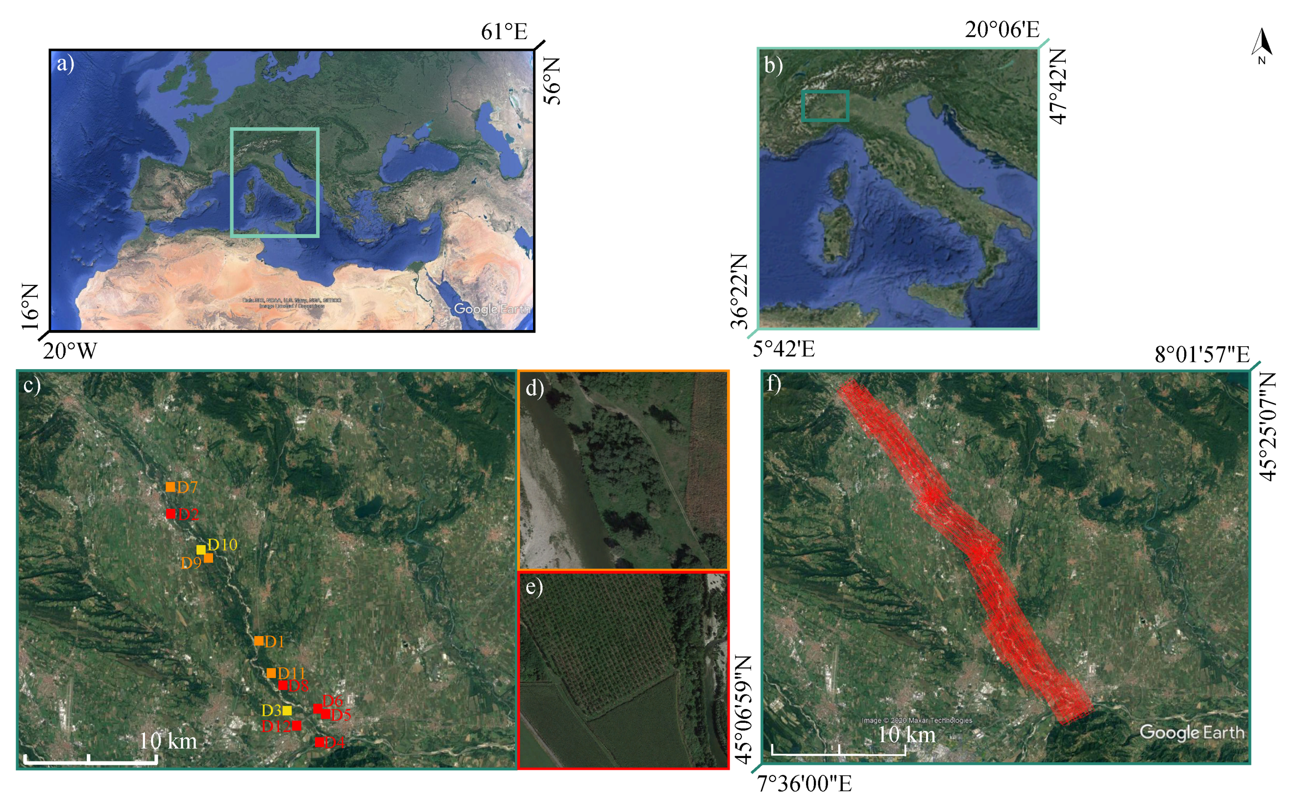
The study areas are located in the Orco River floodplain (Northwestern Italy, 45 ° 14 22.2 N–7 ° 48 45.2 E), as shown in Figure 2a–c.
The Orco River is 89.57 km long and has a catchment area of 930 km2, bounded by the Gran Paradiso National Park, the Stura di Lanzo Valley, the Vanoise National Park, and the Canavese Valley at the Northern, Southern, Western, and Eastern side, respectively. The Orco River floodplain is characterized by a low degree of anthropic activities so that the river channels and meanders can migrate over time. The study sites are located between the town of Cuorgnè and the confluence with the Po River and are occupied by stands of deciduous trees, mainly poplars (Populus alba, Populus nigra), willows (Salix alba), black locusts (Robinia pseudoacacia), oaks (Quercus robur), and hornbeams (Carpinus betulus). Some of these stands belong to commercial plantations and are characterized by well-separated trees of similar age and size and organized according to a regular pattern, such as at the study area hereinafter called D 2 (Figure 2e). Nevertheless, the majority of vegetation follows the natural life cycle of the riparian forests, being populated by trees of different sizes and ages, randomly arranged, often with partially-overlapping crowns. An example of this latter case is shown by the study area hereinafter called D 1 (Figure 2d). Table 1 reports the main features of the twelve study areas. No significant topographic variations are reported for the selected areas since they are generally flat or with very gentle slope (average slope range from 1 to 5 degrees except for D 7 , which is close to the river banks).
The LiDAR data associated with these study areas were acquired on 28 February 2019 by the Italian National Council of Research—Research Institute for Geo-Hydrological Protection (CNR-IRPI) with a LiteMapper 6800 installed on a POD DART certificated by EASA with a minor/STC approval for Eurocopter AS350 Heliwest. The scanning process was designed to guarantee: (i) a raw coverage of the twelve surveyed areas equal to nine points·m 2 on average; (ii) a minimal stereoscopic coverage equal to 60% and 30% for the forward and sideward overlap between adjacent swaths, respectively, and (iii) an average ground sampling distance equal to 10 cm/pixel. The scan frequency was 400 KhZ, whereas the flight height ranged between 675 and 794 m above sea level. The scan angle ranges from 4 ° to 19 ° , approximately, for the study areas. The trajectories of the flight are shown in Figure 2f. The dataset was provided as two separate clouds for the ground and the vegetation, respectively.
During the LiDAR data acquisition, the authors carried out a tree census within the study areas. The tree coordinates were taken by means of a Real-Time Kinematic Global Positioning System (RTK-GPS), model ROVER LEICA 1250, and GNSS smart antenna. The error position of this device is approximately 1.0 m when performing measurements within the tree stands because of the reduced availability of satellites for the GNSS-based positioning and the low signal from the reference station for the kinematic corrections. After the survey, the acquired tree positions were double-checked with a visual inspection of the orthophotos deriving from the LiDAR campaign.

2.2. Presentation of the Algorithm

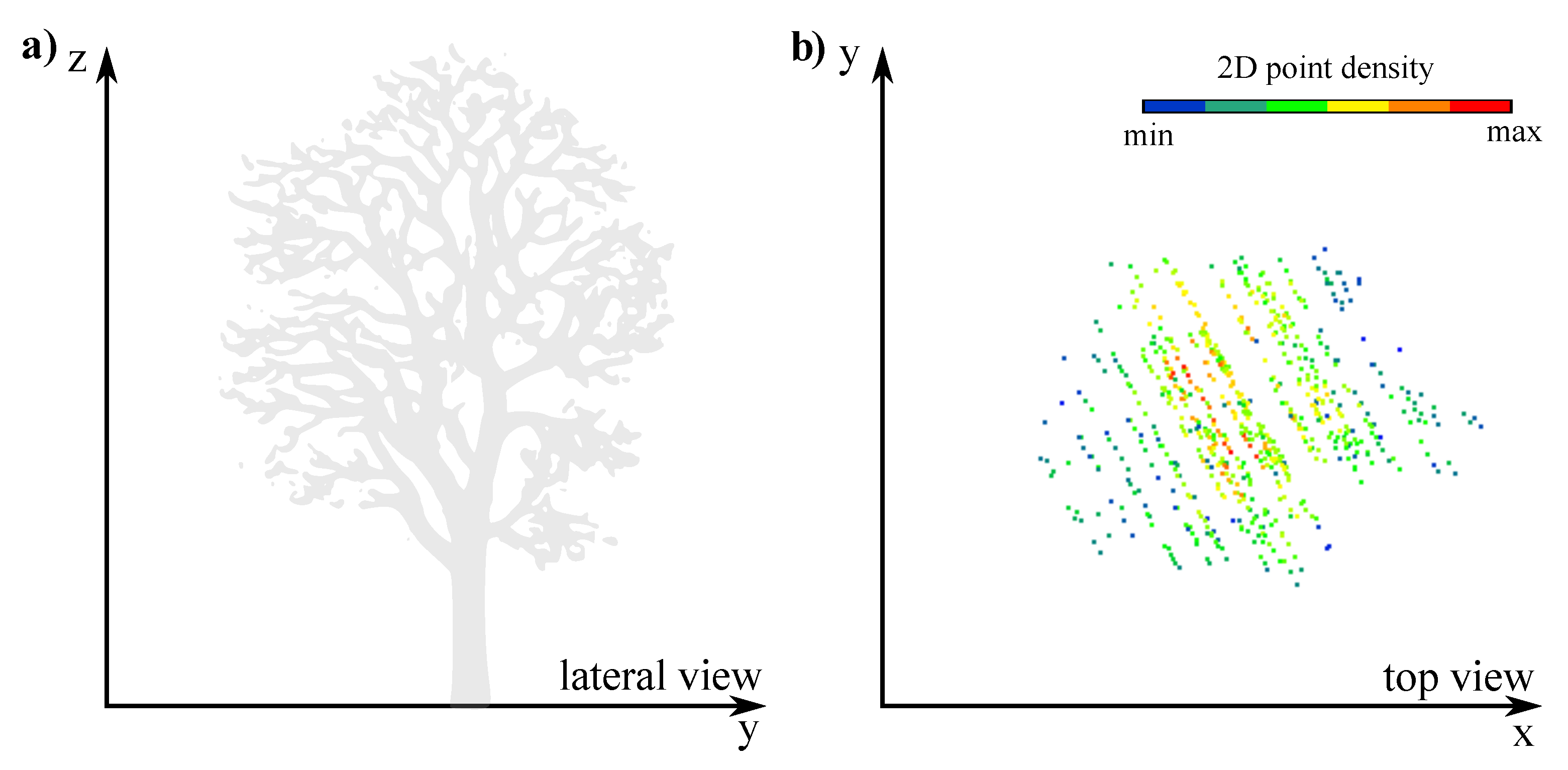
The algorithm is provided in Matlab® code and freely available in the supplementary material. Unlike most of the other existing methods, it does not look for local height maxima but local point density maxima, after having defined the point density as the number of the points’ projections on the plane z = 0 per unit area. The underlying assumption is that the point cloud becomes denser in correspondence with the tree center. Thus, the principles upon which the algorithm is based are that: (i) in the lower layers, LiDAR systems tend to record the highest number of returns when the signal intercepts tree trunks unless too thick understory vegetation is present, and (ii) above a certain reference height the density of tree branches is higher at the center of the crown, decreasing towards its edges. Whereas the former statement is intuitive, the latter has been confirmed by previous studies e.g., [49,64,65], which have also reported that this feature does not depend on the crown shape. Accordingly, this assumption holds for LiDAR data acquired in leaf-off conditions, such as the ones used in this work. We further checked the validity of this hypothesis, by projecting all the points of the cloud on the plane z = 0 and computing their areal density. As it can be observed in Figure 3, the density is maximum at the tree center and gradually decreases towards the tree edges.
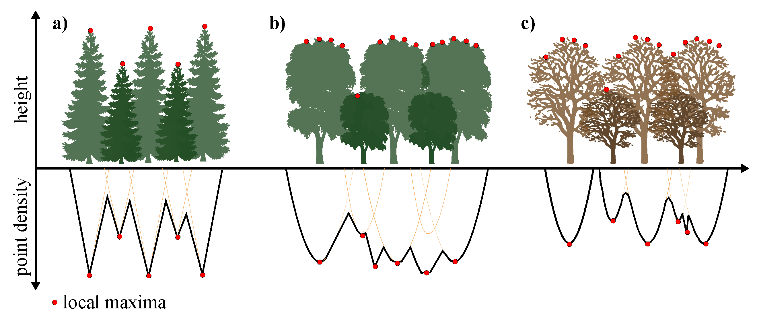
The adoption of a density-based approach allows the algorithm to overcome the limitations of the other approaches when applied to deciduous stands. The upper panels of Figure 4 provide a graphical explanation of the influence that the spatial distribution of the trees has on their detection when the local height maxima are looked for, whereas the lower panels highlight the intrinsic advantage of the density-based approaches.

2.2.1. Pre-Processing

The required input is a text file containing the { x , y , z } coordinates of the elements constituting the LiDAR point-cloud, where the vertical coordinate z must be expressed as relative height with respect to the ground. The generation of the ground surface model and the computation of the relative heights is required prior to the use of the algorithm.

2.2.2. Workflow

Firstly, the algorithm removes the outliers from the point cloud that are associated with unrealistic vertical coordinates, as well as the points lower than 1.4 m, which may be associated with shrubs, bushes, and grasses. In this way, the computational time is reduced.
Secondly, for each point of the ‘cleaned’ cloud, the algorithm computes the most frequent radius, which is a proxy of the crown radius. To this aim, it sorts the inverse distances from all the surrounding points, applies the periodogram method to obtain the Fourier transform of the inverse distance signal, and switches from the space to frequency domain. The computation of the power spectral density of this signal leads to the identification of the mean spatial frequency of the points, which is the inverse of the most frequent radius.
As the computation of the most frequent radius can be time-consuming for large clouds, the input file is clipped around the i-th considered point, at a distance equal to R i . Then, the algorithm determines the areal density D i according to
D i = N i 4 R i 2
For the i-th considered point, N i is the number of the points’ projections on the plane z = 0 that are contained in an area of radius R i . Finally, the algorithm selects the point associated with the maximum density for each A i , and generates a list of the coordinates of the detected stems. The outcome is further refined by applying a filter that eliminates double-counting, based on the typical spacing of stems.
The highest point density corresponds to the stem location, but it does not always coincide with the location of the treetop. Optionally, the algorithm detects the closest local height maximum for each stem and creates a new list of coordinates for the treetops’ location and heights. Another (optional) filter identifies trees with an apparent height close to that of other objects (e.g., fences) and decides whether to remove them on the basis of statistical considerations about the surrounding trees (i.e., comparing the mean and standard deviation of the tree heights).
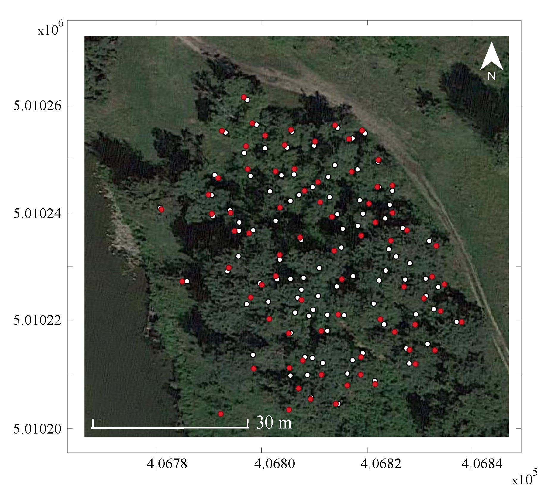
The algorithm’s output can be imported in Geographic Information Systems (GIS) and compared to field data, as shown in Figure 5.
As further discussed in Section 4.3, the present algorithm requires two parameters to be set, namely the radius of the circular area that is used to clip the input file (i.e., R i ), and the critical length for the double-counted stem filter. In this work, we set the clipping radius equal to 20 m, whereas we used an optional function, included in the algorithm, to automatically compute the latter: the critical length can be interpreted as a proxy of the typical stem spacing that can be observed in the study area; therefore, for each detected stems, the function computes the most frequent spacing with respect to the surrounding trees and then sets the critical length as the median of the resulting spacing values.
The conceptual workflow of the algorithm is reported in Figure 6, whereas the technical details about the algorithm setup are reported in Appendix A.

2.3. Accuracy Assessment

The accuracy for the tree count was assessed by following the same criteria adopted in the literature: the algorithm-detected trees were classified as true positive T P if correctly identified, and false positive F P if they do not correspond to the field-mapped ones; the trees omitted by the algorithm were instead classified as false negative F N e.g., [51,57]. The rate of tree detection is represented by the recallr metric, its correctness by the precisionp, and the overall accuracy by the F-score F [77] that were computed as follows:
r = T P T P + F N p = T P T P + F P F = 2 r · p r + p
All of these metrics range from 0 to 1.
The position error, expressed in m, was calculated as the average distance between the field-measured trees and the algorithm-detected ones.
The correct shift from the stem position to the closest height maxima to define the treetops was checked by comparing the resulting stem-to-top distances with the typical values of the crown radius.

2.4. Sensitivity Analysis and the Parameter Setting

As said above, the algorithm requires the setting of two input parameters: (i) the radius of the area to clip the input file around each element, and (ii) the critical length to detect the double-counted stems. We performed an analysis to assess the parameter sensitivity in the outcomes of the algorithm. For this purpose, we tested 10 values of the clipping radius in the range 10–100 m, and twenty values of the critical length in the range 0.5–10.0 m. In case the clipping radius exceeded the extent of the study areas, all of the input points were considered.
As we mentioned in the previous paragraphs, the algorithm can optionally compute the critical length as a proxy of the typical stem spacing on the basis on the statistics of the distances among the identified stems. We tested the effectiveness of this automatic function by comparing the real spacing, obtained by site-specific observations, with the optimal spacing that emerges from the sensitivity analysis and that leads to the highest accuracy, and the values computed by the algorithm.

2.5. Application to Re-Sampled Point Clouds

Finally, we re-tested the presented algorithm on the same study cases but using lower resolution input data. The new datasets were obtained through the random re-sampling of the vegetation point clouds by employing the free software CloudCompare. The rate of point reduction was of 10%, 20%, 30%, 40%, 50%, 60%, 70%, 80%, and 90%, corresponding to an average density of 8.1, 7.2, 6.3, 5.4, 4.5, 3.6, 2.7, 1.8, and 0.9 points·m 2 . This additional test allowed us to understand the influence of point density on the achieved accuracy and to define a minimum requirement for the resolution of the input LiDAR data.

3. Results

3.1. Algorithm Performance

Table 2 compares the real tree count with the algorithm-derived one for all the twelve areas and shows the accuracy metrics, the position error, and the main statistics of the stem-to-top distance.
A scatter plot reporting algorithm detected versus field-detected is displayed in Figure 7a, with a fairly good agreement. The accuracy metrics are also reported in Figure 7b.
The algorithm provided a successful tree count in eight of the twelve sites ( D 3 , D 5 D 9 , D 11 D 12 ,), where the percentage error of the tree count did not exceed the 20%. The recall and precision indices were generally higher than 0.80. The mean overall accuracy of the algorithm outcomes (F-score) is 0.91. This performance is equal to or higher than the existing methods (see [57] for a summary about the achieved accuracy).
In more detail, the lowest recall value was recorded for D 2 (r = 0.58), where many trees are missed because of a local decrease of LiDAR points representing the bare young vegetation in the area. Some trees are represented, in fact, by very few points in the cloud (see Figure 8), therefore precluding the identification of the point density maxima. In D 1 (r = 0.78), some trees were likely lost because of the intense crown interlacing, which misled the detection of local density maxima. As it will be better explained in Section 3.2, the low recall of D 10 (r = 0.79) is due to the presence of two kinds of tree spatial distributions, regular and random that affected the computation of the spacing parameter and the related double-stem removal, leading to an excessive reduction of the tree number.
The lowest precision value was found for D 3 (p = 0.84) and D 4 (p = 0.75). In D 3 , this is likely due to the features of the tree pattern. One portion of D 3 is indeed regular, with equispaced trees that are relatively far between each other. The other portion is characterized by a random tree distribution, with very short and variable stem spacing. This aspect likely altered the algorithm’s assessment of the stem spacing that resulted in being shorter than the effective one in the former portion, thus leading to double-counting some trees. Similarly, the presence of trees of very different size in D 4 affected the stem spacing computation, so that a too short stem spacing led to impair the double-stem removal.
The position error of the algorithm-detected trees is similar to the error of the instrumentation used to perform the tree mapping. The largest error is recorded for D 1 (1.25 m) and is likely due to the intense interlacing of the tree crowns that can move the density maxima from the stem towards the crown edges.
The algorithm can detect the treetops associated with the identified stems. As Table 2 shows, the mean stem-to-top shift is always in the range [0.5–0.8 m] that is lower or close to the minimum crown radius that the literature reports for the species found in the study areas, as well as the maximum shift is largely lower than the average crown radius [78,79]. The minimum shift is equal to 0 for all the areas, meaning that there is always at least one treetop perfectly centered over the stem. These values indicate that the stem-to-top shift worked properly by identifying treetops that effectively belong to the detected stems, as also a visual inspection of results confirmed.

3.2. Sensitivity Analysis Results

The clipping radius affects the computational times, as the higher the clipping radius, the larger the analyzed area (and the number of considered points). Table 3 highlights the direct proportionality between the elapsed time and the number of points that constitute the input point cloud, where elapsed time values refer to the use of a personal computer (RAM 16 GB, processor i7-7700HQ), and the clipping radius is set equal to 20 m.
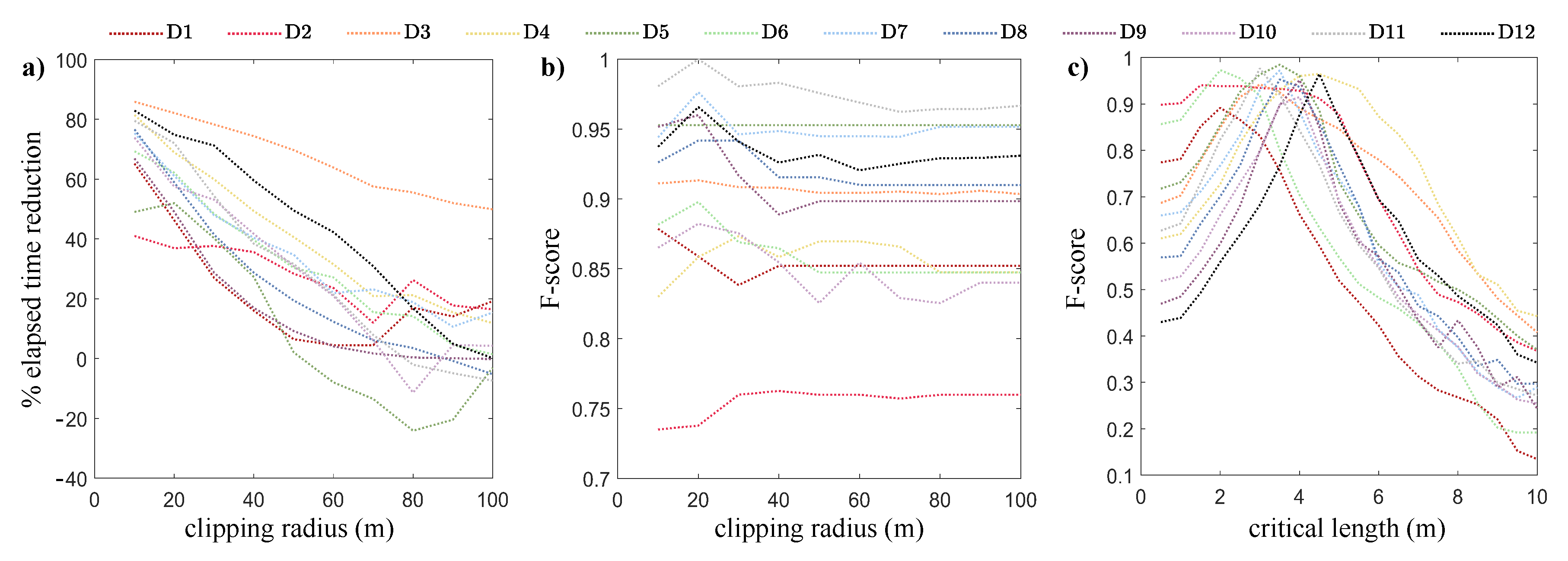
Figure 9a shows the percentage time reduction of the elapsed time with the increasing of the clipping radius. A lower bound of the clipping radius must be around 10–20 m, since at least one tree must be included in the analysis. Since the accuracy is poorly affected by this quantity (see Figure 9b), a value of approximately 20 m is a fair compromise between high accuracy and low computational times for both regular and random stands.
The setting of the critical length allows the algorithm to eliminate false double detection, namely the stems that are too close to each other to belong to two different plants. Therefore, it is defined as the typical spacing between stems within a stand. Figure 9c shows that the accuracy is highly dependent on this parameter. High accuracy is met for critical lengths between 2 and 6 m, which is consistent with the values observed in the study areas, as shown in columns 2 and 3 of Table 4.
This result highlights that the algorithm can achieve high accuracy when the correct tree spacing is set, thus suggesting a significant site-dependency and the need for field surveys to measure it. In order to overcome this limitation, we included an optional function that allows the algorithm to quantify this parameter in the case that the average stem spacing is not known. Table 4 highlights an overall agreement between real, optimal, and computed values. A few exceptions are: (i) D 2 for which computed and real spacing perfectly agree although they are not associated with the best accuracy (albeit higher than 0.80); D 4 and D 5 , which are both characterized by a large minimum spacing (5 and 8 m, respectively). In this latter case, both the optimal and computed spacing do not match the actual spacing but the tree crown radius, nevertheless giving F-score values higher than 0.80.

3.3. Re-Sampling Results

The elapsed time is directly proportional to the number of points that constitute the input point cloud (see Table 3). Consequently, the point cloud re-sampling leads to the proportional reduction of the elapsed time, as Figure 10a highlights.
The F-score remains almost steady up to a re-sampling of the 80%, as Figure 10b shows. Within this range of the re-sampling rate, the slight fluctuations (never exceeding 0.1) of the F-score are related to the randomness that drives the re-sampling process. F-score increments indicate that the re-sampling led to a cleaning of the point cloud with respect to the overlapping crown, thus making the stems more evident. Analogously, F-score reductions indicate that the random point removal jeopardizes the stem identification by reducing the point density closer to the stem than at the crown edges. When the re-sampling rate exceeds 80%, the F-score drastically reduces for eight of the twelve investigated areas, whereas it increases for D 3 , D 4 , D 9 , and D 11 , which presents extremely interlaced crowns both for regular ( D 4 , and part of D 3 ) and random ( D 9 , D 11 ) tree patterns. In terms of point density, these results translate into accuracy larger than 0.70 for cloud as dense as (or denser than) 2 points·m 2 .
As the F-score reduces the position error increases, therefore, the more intense the re-sampling the higher the position error, as Figure 10c shows.

4. Discussion

4.1. Data for the Algorithm’s Application

The presented algorithm was designed to process ALS-derived point clouds. Although photogrammetry can also be used for the generation of point clouds, its products are not suitable for the algorithm’s application. Photogrammetric point clouds derive from image processing and represent the top layer of the objects that stand on the ground surface. In case of forested areas, they can be used to interpolate the canopy surface but do not provide information about the under-canopy vegetation structures and the topography [11,80,81,82], which are instead necessary for the correct implementation of the algorithm.
The algorithm was not tested on Terrestrial Laser Scanning (TLS) point clouds because of the non-availability of that kind of data for the study area. However, we presume that the application to TLS may not be convenient: although the underlying hypothesis may hold (e.g., the areal point density of the cloud’s projection of the z = 0 axis is higher at the stem locations and decrease towards the crown edges), the extremely high point density of the TLS datasets could remarkably increase the computational time. For these reasons, we encourage the use of one of the method that the literature provides e.g., [72,73,74,75] when dealing with TLS data.

4.2. Achieved Accuracy and the Influence of Data Quality

The presented algorithm provided a high accuracy tree count both in regular-patterned plantation and stands where the trees naturally established according to a random spatial distribution. The detection of individual trees is easier for regular stands, as the point cloud itself already indicates the potential individual elements, as occurs in D 12 -like areas. Nevertheless, the algorithm demonstrated good performance also in random areas, where the point cloud itself does not provide any indication of the individual trees and the visual inspection of orthophotos can be misleading, as for D 1 -like areas.
The count error has a slight correlation to the areal extent of the study stands. In addition, the recall and precision metrics often reduce when the algorithm deals with heterogeneous areas (both in terms of spatial tree distribution and tree size or age). These results suggest that the individual tree detection may be improved by previously subdividing the study site into areas of homogeneous features according to field observations or visual inspection of satellite images and orthophotos.
The mean shift from the stem to the treetop location is usually lower than the minimum crown radius of the tree species that can be found within the study areas, indicating that the algorithm correctly associates the stems with their corresponding treetops.
The position error of the detected trees is generally similar to that of the instrumentation used to map the trees within the stand (1.0 m). However, it must be noted that, because of the nadir or small off-nadir scan angle and the flight conditions, the available cloud consists of point arranged almost regularly according to a three-dimensional grid. As Figure 3 clearly shows, the top view of the acquired LiDAR point clouds results in a linear pattern where the lines, perpendicular to the flight trajectory, have an average distance of 0.5 m. Therefore, an additional error of ±0.25 m should be considered in this case.
The influence of the scan angle in LiDAR-derived tree structures is still debated in the literature. Some studies have indeed demonstrated that the accuracy of canopy height and other vegetation parameters decreases with off-nadir angle [83]. Large scan angles also result in shadow areas where the pulses do not penetrate adjacent tree crowns [84,85], and, generally, the higher the scan angle the lower the returns from the ground because of an increment of the tree crown projection to the near nadir crown area [83,84,86,87]. The influence of scan angle is related to the spatial configurations of the trees: it becomes stronger as the crown height exceeds the crown width (e.g., in coniferous stands) and when the number of stems per unit area decreases [87].
With respect to the presented algorithm, the nadiral signal may provide fewer returns than those obtained in off-nadir conditions, as the literature suggests [88]. Although our data indicate no correlation between scan angle and point density, we note that an overall point density reduction is not expected for the performance of the algorithm unless the point density becomes lower than 2 points·m 2 , as shown in Section 3.3. Not even the three-dimensional point pattern seems to impact the tree count since the algorithm looks for local maxima of the areal point density by inspecting areas whose radius largely exceeds the distance between the pattern’s lines.
The stand features (e.g., rounded-shaped crowns and high stems per unit areas) and the nadir or small off-nadir acquisition suggest a low influence of the scan angle in the study areas for what concerns the height accuracy. However, it is known that the LiDAR tends to underestimate the tree height [17,89], especially when the point density decreases [90,91]. The laser beam may not be intercepted by the highest branches, and this effect may be exacerbated by leaf-off conditions [92,93]. Moreover, the trees often lean while growing, thus aggravating the height underestimation. Because of the aforementioned reasons, the LiDAR-derived treetop heights that our algorithm provides should be calibrated on the basis of field measurements prior to their use, as it is common practice for LiDAR applications in forestry e.g., [17].
As mentioned in Section 2, the available LiDAR data already consisted of separated point clouds for the ground and the vegetation, respectively. Moreover, the topographic flatness of the study site allowed for a straightforward interpolation of the ground surface that is necessary to compute the relative heights of the vegetation cloud. Complex topographies do not directly hamper the algorithm, which just works on the vegetation point cloud, but can indirectly impair the tree identification by affecting the classification of vegetation and ground points and the following ground surface interpolation [94]. However, despite the potential inaccuracy of ground interpolation in complex topographies, the methods to be adopted for the surface interpolation are not the object of this work and have been extensively discussed in other research e.g., [89,94].

4.3. The Influence of the Parameter Setting

The CHM methods are highly influenced by the parameter setting. For instance, Chen et al. [32] describes their extreme sensitivity to the size of the cell window that is used to inspect the CHM and detect the height maxima. The window size, indeed, represents the main and most critical parameter to achieve satisfactory accuracy. A large window smooths the variations of canopy height and drastically reduces the detected peaks, whereas a small one can dramatically increase the number of peaks. The literature does not provide robust criteria for the window size setting and, therefore, the CHM-methods require site-specific measurements and calibration [28,30,36].
The cloud-based methods need a proper parameter setting too. For instance, the tools that ground on the works of Ayrey et al. [62], Rahman and Gorte [64] identify the crown center by inspecting the point density within vertical cylinders of arbitrary size and generating a density raster that shows the density peaks e.g., [95]. The cylinder radius has to be close to the typical tree spacing, whereas the issue of the cell size setting resembles that of the CHM-based methods. Large cells excessively smooth the density raster and small ones overestimate the peaks so that the literature suggests values of the same order of magnitude of 1/(point density)0.5 [32].
Similarly to the other methods, the proposed algorithm requires a set of input parameters. Nevertheless, it has the advantage to achieve satisfying accuracy (F-score > 0.70) also with the default setting. This setting comprises a clipping radius equal to 20 m that, as the sensitivity analysis highlights, does not affect the results but strongly speeds up the tree identification process. Moreover, it comprises the automatic estimation of the typical stem spacing from the point cloud features, which reduces the dependency from costly and time-consuming site-specific surveys.
The default setting also includes a threshold to remove outliers above 40 m from the input point cloud. This threshold was not considered for the sensitivity analysis as its influence is negligible if realistic values are used (e.g., 40 m is the height limit for the species found in the study area). We refer the reader to Appendix A for further details.

4.4. Cloud Re-Sampling and Low-Resolution Data

The results shown in Section 3.3 highlight the linear relationship between computational time and input point number. The performance refers to the features of a personal computer without the implementation of parallelization techniques, and the order of magnitude of the elapsed time is that of minutes due to the relatively small size of the investigated areas. The use of the algorithm for input clouds characterized by millions of points would require long computation time. Therefore, future works will focus on its parallelization and application to large domains.
The results shown in Section 3.3 suggest that the algorithm can be applied also to very low-resolution input clouds since it is able to provide F-scores higher than 0.70 also for point densities of 2.0 points·m 2 . This means that, in the case of large datasets, the user can re-sample the original point cloud to create one of lower density and, consequently, drastically reduce the computational effort.
The chance to effectively work with low-density point clouds allows the algorithm’s user to carry out analyses of data provided by a wide range of LiDAR devices, therefore avoiding the use of expensive and advanced equipment. In addition, although LiDAR measurements for forestry purposes are often scheduled under leaf-on conditions, topographic surveys are often carried out in leaf-off conditions. This implies a few points representing deciduous trees. It is clear that, for this particular case, the capability of the presented algorithm to deal with low-density clouds becomes very important. The proposed algorithm can, therefore, analyze old point-clouds, whose density is usually lower than the most recent ones, thus providing time series of tree position and features. This information can constitute a valuable contribution to forest modeling and management.
It is worth mentioning that the results indicate an increment in the position error as the point density reduces. Thus, although the re-sampling could speed up the algorithm’s computation without impairing the tree count, it should be avoided when an accurate localization of the detected trees is the main target of the LiDAR data processing.

5. Conclusions

In this work, we proposed a novel algorithm for the identification of individual trees in forest stands from three-dimensional point clouds. The algorithm is designed to process airborne LiDAR point clouds and grounds on the detection of stems according to local maxima of the areal point density. It can give the stem coordinates and the treetop height as output.
The algorithm achieves high accuracy when applied to stands with both regular and random spatial tree distribution. The achieved F-score is higher than 0.70 and position error close to 1.0 m, if the input point cloud has a density of at least 2 points·m 2 . Thanks to its capability to deal with relatively low-density clouds, old LiDAR datasets can be also accurately analyzed, while very dense clouds can be sub-sampled to speed up the process.
A sensitivity analysis highlighted the influence that the parameter describing the critical stem spacing has on the achieved accuracy. However, the algorithm demonstrated to be able to automatically compute it on the basis of statistical considerations about the geometric configuration of the detected trees. This feature allows the algorithm to also be adopted with little information about the study area.
The main advantages and limitations of the algorithm are summarized in Table 5 along with the precautions that may be taken to obtain better results.
Despite its simplicity, the algorithm can constitute the basis for more complex tools, such as those for crown segmentation. In addition, it may allow for the biomass estimation if coupled to GIS information about the spatial distribution of tree species and site-dependent allometric laws. There are many applications for such a coupled methodology, ranging from forest inventories e.g., [25,96] to the characterization of riparian vegetation for hydrodynamic modeling e.g., [97,98,99].
Our results suggest that the accuracy of tree identification relies on the quality of the input point clouds. Although this is not a limitation of the algorithm itself, it must be considered when analyzing the region of interest. It is worth noting that the algorithm performs better in plantations and forest stands with mature vegetation since the mature trees are better represented in the point clouds and generally more spaced apart from each other. The application of the algorithm to natural stands is generally good unless the stem spacing is excessively variable or the crown is very interlaced. We also point out that the presence of high and thick brambles, as often occurs in the riparian zone, can decrease the algorithm accuracy since they may be wrongly identified as trees.
Finally, we note that the algorithm was tested on LiDAR data acquired during leaf-off conditions. Because of a density-based approach, the algorithm is expected to work well in leaf-on conditions too, if applied to coniferous stands (see Figure 4). In that specific case, indeed, the underlying hypothesis (i.e., the correspondence between the maximum point density and the tree center) still holds thanks to the conical shape of these species. Future works should verify whether this hypothesis holds for point clouds acquired in deciduous stands with leaf-on conditions and whether the presence of interlacing branches or their non-symmetric distribution can mislead the stem identification, as is suggested by some authors e.g., [64] and the large position error of D 1 .

Supplementary Materials

The following are available online at https://www.mdpi.com/2072-4292/13/2/322/s1. The supplementary material of this manuscript comprises Table S1 that lists the methods described in the literature (2001–2019) for the identification of individual trees starting from LiDAR data.

Author Contributions

Conceptualization: M.L., F.S. and C.C.; Methodology, Software and Validation: M.L. and F.S.; Writing—Original Draft Preparation: M.L.; Writing—Review and Editing: C.C.; Visualization: F.S.; Supervision and Funding Acquisition: C.C. All authors have read and agreed to the published version of the manuscript.

Funding

This research was partially funded by Regione Piemonte, Settore Difesa del Suolo.

Institutional Review Board Statement

Not applicable

Informed Consent Statement

Not applicable

Data Availability Statement

The data and the algorithm presented in this study are openly available in Zenodo repository at https://doi.org/10.5281/zenodo.4421030.

Acknowledgments

The authors are grateful to the GMG—Geohazard Monitoring Group of CNR—IRPI (Italy) that produced and provided the LiDAR data used in this work. The authors also thank Camilla Redoglia for her contribution during the field surveys.

Conflicts of Interest

The authors declare no conflict of interest.

Abbreviations

The following abbreviations are used in this manuscript:
ALSAirborne Laser Scanning
CHMCanopy Height Model
GISGeographic Information System
GPSGlobal Positioning System
LiDARLight Detection And Ranging
RTKReal Time Kinematic
TLSTerrestrial Laser Scanning

Appendix A. Algorithm Setup

The code has been set to run with default parameters that, as shown in this manuscript, lead to satisfactory accuracy. However, the algorithm also provides a dialog box through which the user can customize it. In this way, site-specific requirements (e.g., the presence of anthropic objects or outliers) can be met.
In the following, the parameters (and their default values) are listed: (i) the upper limit of the height range (default value is 40 m, higher points are removed); (ii) the clipping radius (default value is 20 m); (iii) the critical length for double-stem detection (the default value is self-computed); (iv) the user can decide either to obtain the stem locations only or even treetops and heights (the latter option is usually preferred when the aim is to obtain the tree features or to compute the biomass according to allometric relationships); (v) optionally, the user can specify the height interval of not-natural objects that must be filtered out, e.g., fences (default value is null, but one or more height intervals can be set).
If the last option is chosen, the algorithm identifies the tree (or trees) whose height belongs to the specified interval and assesses if this height is statistically similar to those of the surrounding trees. If the height of the investigated tree does not fall within the interval (mean value ± 2 times the standard deviation), it is considered as an outlier and removed from the list of the identified trees.
This filter is recommended only where the presence of non-natural objects is well-known. In this work, for instance, it could be used when analyzing D 4 and D 7 , where a warehouse 2.0 m high and a fence 2.5 m high were found, respectively. As Figure A1 shows, the warehouse was filtered out by setting the height interval 1.5–2.0 m, whereas the fence by setting 2.0–2.5 m, where the lower values account for the potential underestimation of the LiDAR-derived heights [17,89].
Figure A1. Detected treetops before (black dots) and after (cyan dots) the application of the filter to remove not-natural objects in D 4 and D 7 .
Remotesensing 13 00322 g0a1

References

  1. Flood, M. Laser altimetry: From science to commerical lidar mapping. Photogramm. Eng. Remote Sens. 2001, 67, 1209–1211, 1213–1217. [Google Scholar]
  2. Lindberg, E.; Holmgren, J. Individual tree crown methods for 3D data from remote sensing. Curr. For. Rep. 2017, 3, 19–31. [Google Scholar] [CrossRef] [Green Version]
  3. Andújar, D.; Escolà, A.; Rosell-Polo, J.R.; Fernández-Quintanilla, C.; Dorado, J. Potential of a terrestrial LiDAR-based system to characterise weed vegetation in maize crops. Comput. Electron. Agric. 2013, 92, 11–15. [Google Scholar] [CrossRef] [Green Version]
  4. Eitel, J.U.; Magney, T.S.; Vierling, L.A.; Brown, T.T.; Huggins, D.R. LiDAR based biomass and crop nitrogen estimates for rapid, non-destructive assessment of wheat nitrogen status. Field Crops Res. 2014, 159, 21–32. [Google Scholar] [CrossRef]
  5. Reutebuch, S.E.; McGaughey, R.J.; Andersen, H.E.; Carson, W.W. Accuracy of a high-resolution lidar terrain model under a conifer forest canopy. Can. J. Remote Sens. 2003, 29, 527–535. [Google Scholar] [CrossRef]
  6. Klemas, V. Beach profiling and LIDAR bathymetry: An overview with case studies. J. Coast. Res. 2011, 27, 1019–1028. [Google Scholar] [CrossRef]
  7. Vastaranta, M.; Kantola, T.; Lyytikäinen-Saarenmaa, P.; Holopainen, M.; Kankare, V.; Wulder, M.A.; Hyyppä, J.; Hyyppä, H. Area-based mapping of defoliation of Scots pine stands using airborne scanning LiDAR. Remote Sens. 2013, 5, 1220–1234. [Google Scholar] [CrossRef] [Green Version]
  8. Means, J.E.; Acker, S.A.; Fitt, B.J.; Renslow, M.; Emerson, L.; Hendrix, C.J. Predicting forest stand characteristics with airborne scanning lidar. Photogramm. Eng. Remote Sens. 2000, 66, 1367–1372. [Google Scholar]
  9. Li, Y.; Andersen, H.E.; McGaughey, R. A comparison of statistical methods for estimating forest biomass from light detection and ranging data. West. J. Appl. For. 2008, 23, 223–231. [Google Scholar] [CrossRef] [Green Version]
  10. Dalponte, M.; Reyes, F.; Kandare, K.; Gianelle, D. Delineation of individual tree crowns from ALS and hyperspectral data: A comparison among four methods. Eur. J. Remote Sens. 2015, 48, 365–382. [Google Scholar] [CrossRef] [Green Version]
  11. White, J.C.; Wulder, M.A.; Vastaranta, M.; Coops, N.C.; Pitt, D.; Woods, M. The utility of image-based point clouds for forest inventory: A comparison with airborne laser scanning. Forests 2013, 4, 518–536. [Google Scholar] [CrossRef] [Green Version]
  12. Koch, B.; Heyder, U.; Weinacker, H. Detection of individual tree crowns in airborne lidar data. Photogramm. Eng. Remote Sens. 2006, 72, 357–363. [Google Scholar] [CrossRef] [Green Version]
  13. Chen, Q. Airborne lidar data processing and information extraction. Photogramm. Eng. Remote Sens. 2007, 73, 109. [Google Scholar]
  14. Andersen, H.E.; Reutebuch, S.E.; Schreuder, G.F. Automated individual tree measurement through morphological analysis of a LIDAR-based canopy surface model. In Proceedings of the 1st International Precision Forestry Symposium, Seattle, WA, USA, 17–20 June 2001; pp. 11–21. [Google Scholar]
  15. Lee, A.C.; Lucas, R.M. A LiDAR-derived canopy density model for tree stem and crown mapping in Australian forests. Remote Sens. Environ. 2007, 111, 493–518. [Google Scholar] [CrossRef]
  16. Coomes, D.A.; Dalponte, M.; Jucker, T.; Asner, G.P.; Banin, L.F.; Burslem, D.F.; Lewis, S.L.; Nilus, R.; Phillips, O.L.; Phua, M.H.; et al. Area-based vs tree-centric approaches to mapping forest carbon in Southeast Asian forests from airborne laser scanning data. Remote Sens. Environ. 2017, 194, 77–88. [Google Scholar] [CrossRef] [Green Version]
  17. Yu, X.; Hyyppä, J.; Holopainen, M.; Vastaranta, M. Comparison of area-based and individual tree-based methods for predicting plot-level forest attributes. Remote Sens. 2010, 2, 1481–1495. [Google Scholar] [CrossRef] [Green Version]
  18. González-Ferreiro, E.; Diéguez-Aranda, U.; Barreiro-Fernández, L.; Buján, S.; Barbosa, M.; Suárez, J.C.; Bye, I.J.; Miranda, D. A mixed pixel-and region-based approach for using airborne laser scanning data for individual tree crown delineation in Pinus radiata D. Don plantations. Int. J. Remote Sens. 2013, 34, 7671–7690. [Google Scholar] [CrossRef]
  19. Corona, P.; Fattorini, L. Area-based lidar-assisted estimation of forest standing volume. Can. J. For. Res. 2008, 38, 2911–2916. [Google Scholar] [CrossRef] [Green Version]
  20. Magnussen, S.; Næsset, E.; Gobakken, T.; Frazer, G. A fine-scale model for area-based predictions of tree-size-related attributes derived from LiDAR canopy heights. Scand. J. For. Res. 2012, 27, 312–322. [Google Scholar] [CrossRef]
  21. Duncanson, L.; Dubayah, R. Monitoring individual tree-based change with airborne lidar. Ecol. Evol. 2018, 8, 5079–5089. [Google Scholar] [CrossRef]
  22. Rönnholm, P.; Hyyppä, J.; Hyyppä, H.; Haggrén, H.; Yu, X.; Kaartinen, H. Calibration of laser-derived tree height estimates by means of photogrammetric techniques. Scand. J. For. Res. 2004, 19, 524–528. [Google Scholar] [CrossRef]
  23. White, J.C.; Wulder, M.A.; Varhola, A.; Vastaranta, M.; Coops, N.C.; Cook, B.D.; Pitt, D.; Woods, M. A best practices guide for generating forest inventory attributes from airborne laser scanning data using an area-based approach. For. Chron. 2013, 89, 722–723. [Google Scholar] [CrossRef] [Green Version]
  24. Kandare, K.; Ørka, H.O.; Chan, J.C.W.; Dalponte, M. Effects of forest structure and airborne laser scanning point cloud density on 3D delineation of individual tree crowns. Eur. J. Remote Sens. 2016, 49, 337–359. [Google Scholar] [CrossRef] [Green Version]
  25. Hyyppä, J.; Kelle, O.; Lehikoinen, M.; Inkinen, M. A segmentation-based method to retrieve stem volume estimates from 3-D tree height models produced by laser scanners. IEEE Trans. Geosci. Remote Sens. 2001, 39, 969–975. [Google Scholar] [CrossRef]
  26. Persson, A.; Holmgren, J.; Soderman, U. Detecting and measuring individual trees using an airborne laser scanner. Photogramm. Eng. Remote Sens. 2002, 68, 925–932. [Google Scholar]
  27. Brandtberg, T.; Warner, T.A.; Landenberger, R.E.; McGraw, J.B. Detection and analysis of individual leaf-off tree crowns in small footprint, high sampling density lidar data from the eastern deciduous forest in North America. Remote Sens. Environ. 2003, 85, 290–303. [Google Scholar] [CrossRef]
  28. Popescu, S.C.; Wynne, R.H. Seeing the trees in the forest. Photogramm. Eng. Remote Sens. 2004, 70, 589–604. [Google Scholar] [CrossRef] [Green Version]
  29. Heurich, M.; Weinacker, H. Automated tree detection and measurement in temperate forests of central Europe using laser scanning data. Int. Arch. Photogramm. Remote Sens. Spat. Inf. Sci. 2004, 36, 8. [Google Scholar]
  30. Pitkänen, J.; Maltamo, M.; Hyyppä, J.; Yu, X. Adaptive methods for individual tree detection on airborne laser based canopy height model. Int. Arch. Photogramm. Remote Sens. Spat. Inf. Sci. 2004, 36, 187–191. [Google Scholar]
  31. Weinacker, H.; Koch, B.; Heyder, U.; Weinacker, R. Development of filtering, segmentation and modeling modules for lidar and multispectral data as a fundament of an automatic forest inventory system. Int. Arch. Photogramm. Remote Sens. Spat. Inf. Sci. 2004, 36, W2. [Google Scholar]
  32. Chen, Q.; Baldocchi, D.; Gong, P.; Kelly, M. Isolating individual trees in a savanna woodland using small footprint lidar data. Photogramm. Eng. Remote Sens. 2006, 72, 923–932. [Google Scholar] [CrossRef] [Green Version]
  33. Solberg, S.; Naesset, E.; Bollandsas, O.M. Single tree segmentation using airborne laser scanner data in a structurally heterogeneous spruce forest. Photogramm. Eng. Remote Sens. 2006, 72, 1369–1378. [Google Scholar] [CrossRef]
  34. Pang, Y.; Lefsky, M.; Andersen, H.E.; Miller, M.; Sherrill, K. Validation of the ICEsat vegetation product using crown-area-weighted mean height derived using crown delineation with discrete return lidar data. Can. J. Remote Sens. 2008, 34, S471–S484. [Google Scholar] [CrossRef]
  35. Maltamo, M.; Peuhkurinen, J.; Malinen, J.; Vauhkonen, J.; Packalén, P.; Tokola, T. Predicting tree attributes and quality characteristics of Scots pine using airborne laser scanning data. Silva Fenn. 2009, 43, 507–521. [Google Scholar] [CrossRef] [Green Version]
  36. Yu, X.; Hyyppä, J.; Vastaranta, M.; Holopainen, M.; Viitala, R. Predicting individual tree attributes from airborne laser point clouds based on the random forests technique. ISPRS J. Photogramm. Remote Sens. 2011, 66, 28–37. [Google Scholar] [CrossRef]
  37. Ene, L.; Næsset, E.; Gobakken, T. Single tree detection in heterogeneous boreal forests using airborne laser scanning and area-based stem number estimates. Int. J. Remote Sens. 2012, 33, 5171–5193. [Google Scholar] [CrossRef]
  38. Jing, L.; Hu, B.; Li, J.; Noland, T. Automated delineation of individual tree crowns from LiDAR data by multi-scale analysis and segmentation. Photogramm. Eng. Remote Sens. 2012, 78, 1275–1284. [Google Scholar] [CrossRef]
  39. Dalponte, M.; Coomes, D.A. Tree-centric mapping of forest carbon density from airborne laser scanning and hyperspectral data. Methods Ecol. Evol. 2016, 7, 1236–1245. [Google Scholar] [CrossRef] [Green Version]
  40. Silva, C.A.; Hudak, A.T.; Vierling, L.A.; Loudermilk, E.L.; O’Brien, J.J.; Hiers, J.K.; Jack, S.B.; Gonzalez-Benecke, C.; Lee, H.; Falkowski, M.J.; et al. Imputation of individual longleaf pine (Pinus palustris Mill.) tree attributes from field and LiDAR data. Can. J. Remote Sens. 2016, 42, 554–573. [Google Scholar] [CrossRef]
  41. Bian, Y.; Zou, P.; Shu, Y.; Yu, R. Individual tree delineation in deciduous forest areas with LiDAR point clouds. Can. J. Remote Sens. 2014, 40, 152–163. [Google Scholar] [CrossRef]
  42. Hirata, Y.; Furuya, N.; Suzuki, M.; Yamamoto, H. Airborne laser scanning in forest management: Individual tree identification and laser pulse penetration in a stand with different levels of thinning. For. Ecol. Manag. 2009, 258, 752–760. [Google Scholar] [CrossRef]
  43. Duncanson, L.; Cook, B.; Hurtt, G.; Dubayah, R. An efficient, multi-layered crown delineation algorithm for mapping individual tree structure across multiple ecosystems. Remote Sens. Environ. 2014, 154, 378–386. [Google Scholar] [CrossRef]
  44. Zhao, D.; Pang, Y.; Li, Z.; Liu, L. Isolating individual trees in a closed coniferous forest using small footprint lidar data. Int. J. Remote Sens. 2014, 35, 7199–7218. [Google Scholar] [CrossRef]
  45. Kwak, D.A.; Lee, W.K.; Lee, J.H.; Biging, G.S.; Gong, P. Detection of individual trees and estimation of tree height using LiDAR data. J. For. Res. 2007, 12, 425–434. [Google Scholar] [CrossRef]
  46. Leckie, D.; Gougeon, F.; Hill, D.; Quinn, R.; Armstrong, L.; Shreenan, R. Combined high-density lidar and multispectral imagery for individual tree crown analysis. Can. J. Remote Sens. 2003, 29, 633–649. [Google Scholar] [CrossRef]
  47. Falkowski, M.J.; Smith, A.M.; Hudak, A.T.; Gessler, P.E.; Vierling, L.A.; Crookston, N.L. Automated estimation of individual conifer tree height and crown diameter via two-dimensional spatial wavelet analysis of lidar data. Can. J. Remote Sens. 2006, 32, 153–161. [Google Scholar] [CrossRef] [Green Version]
  48. Wu, B.; Yu, B.; Wu, Q.; Huang, Y.; Chen, Z.; Wu, J. Individual tree crown delineation using localized contour tree method and airborne LiDAR data in coniferous forests. Int. J. Appl. Earth Obs. Geoinf. 2016, 52, 82–94. [Google Scholar] [CrossRef]
  49. Rahman, M.; Gorte, B. Tree crown delineation from high resolution airborne lidar based on densities of high points. In Proceedings of the ISPRS Workshop Laserscanning 2009, ISPRS XXXVIII (3/W8), Paris, France, 1–2 September 2009. [Google Scholar]
  50. Richardson, J.J.; Moskal, L.M. Strengths and limitations of assessing forest density and spatial configuration with aerial LiDAR. Remote Sens. Environ. 2011, 115, 2640–2651. [Google Scholar] [CrossRef]
  51. Li, W.; Guo, Q.; Jakubowski, M.K.; Kelly, M. A new method for segmenting individual trees from the lidar point cloud. Photogramm. Eng. Remote Sens. 2012, 78, 75–84. [Google Scholar] [CrossRef] [Green Version]
  52. Hu, B.; Li, J.; Jing, L.; Judah, A. Improving the efficiency and accuracy of individual tree crown delineation from high-density LiDAR data. Int. J. Appl. Earth Obs. Geoinf. 2014, 26, 145–155. [Google Scholar] [CrossRef]
  53. Mongus, D.; Žalik, B. An efficient approach to 3D single tree-crown delineation in LiDAR data. ISPRS J. Photogramm. Remote Sens. 2015, 108, 219–233. [Google Scholar] [CrossRef]
  54. Reitberger, J.; Schnörr, C.; Krzystek, P.; Stilla, U. 3D segmentation of single trees exploiting full waveform LIDAR data. ISPRS J. Photogramm. Remote Sens. 2009, 64, 561–574. [Google Scholar] [CrossRef]
  55. Holmgren, J.; Lindberg, E. Tree crown segmentation based on a geometric tree crown model for prediction of forest variables. Can. J. Remote Sens. 2013, 39, S86–S98. [Google Scholar] [CrossRef]
  56. Holmgren, J.; Lindberg, E. Tree crown segmentation based on a tree crown density model derived from Airborne Laser Scanning. Remote Sens. Lett. 2019, 10, 1143–1152. [Google Scholar] [CrossRef]
  57. Lu, X.; Guo, Q.; Li, W.; Flanagan, J. A bottom-up approach to segment individual deciduous trees using leaf-off lidar point cloud data. ISPRS J. Photogramm. Remote Sens. 2014, 94, 1–12. [Google Scholar] [CrossRef]
  58. Morsdorf, F.; Meier, E.; Kötz, B.; Itten, K.I.; Dobbertin, M.; Allgöwer, B. LIDAR-based geometric reconstruction of boreal type forest stands at single tree level for forest and wildland fire management. Remote Sens. Environ. 2004, 92, 353–362. [Google Scholar] [CrossRef]
  59. Tiede, D.; Hochleitner, G.; Blaschke, T. A full GIS-based workflow for tree identification and tree crown delineation using laser scanning. In Proceedings of the ISPRS Workshop CMRT, Vienna, Austria, 29–30 August 2005; Volume 5. [Google Scholar]
  60. Lee, H.; Slatton, K.C.; Roth, B.E.; Cropper, W., Jr. Adaptive clustering of airborne LiDAR data to segment individual tree crowns in managed pine forests. Int. J. Remote Sens. 2010, 31, 117–139. [Google Scholar] [CrossRef]
  61. Véga, C.; Hamrouni, A.; El Mokhtari, S.; Morel, J.; Bock, J.; Renaud, J.P.; Bouvier, M.; Durrieu, S. PTrees: A point-based approach to forest tree extraction from lidar data. Int. J. Appl. Earth Obs. Geoinf. 2014, 33, 98–108. [Google Scholar] [CrossRef]
  62. Ayrey, E.; Fraver, S.; Kershaw, J.A., Jr.; Kenefic, L.S.; Hayes, D.; Weiskittel, A.R.; Roth, B.E. Layer stacking: A novel algorithm for individual forest tree segmentation from LiDAR point clouds. Can. J. Remote Sens. 2017, 43, 16–27. [Google Scholar] [CrossRef]
  63. Ma, Z.; Pang, Y.; Wang, D.; Liang, X.; Chen, B.; Lu, H.; Weinacker, H.; Koch, B. Individual Tree Crown Segmentation of a Larch Plantation Using Airborne Laser Scanning Data Based on Region Growing and Canopy Morphology Features. Remote Sens. 2020, 12, 1078. [Google Scholar] [CrossRef] [Green Version]
  64. Rahman, M.; Gorte, B. Individual tree detection based on densities of high points of high resolution airborne LiDAR. In Proceedings of the GEOBIA, 2008—Pixels, Objects, Intelligence: GEOgraphic Object Based Image Analysis for the 21st Century, Calgary, AB, Canada, 5–8 August 2008; University of Calgary: Calgary, AB, Canada, 2008; pp. 350–355. [Google Scholar]
  65. Rahman, M.; Gorte, B. Tree filtering for high density airborne LiDAR data. In Proceedings of the International Conference on LiDAR Applications in Forest Assessment and Inventory, Edinburgh, UK, 17–19 September 2008. [Google Scholar]
  66. Ferraz, A.; Bretar, F.; Jacquemoud, S.; Gonçalves, G.; Pereira, L.; Tomé, M.; Soares, P. 3-D mapping of a multi-layered Mediterranean forest using ALS data. Remote Sens. Environ. 2012, 121, 210–223. [Google Scholar] [CrossRef]
  67. Paris, C.; Valduga, D.; Bruzzone, L. A hierarchical approach to three-dimensional segmentation of LiDAR data at single-tree level in a multilayered forest. IEEE Trans. Geosci. Remote Sens. 2016, 54, 4190–4203. [Google Scholar] [CrossRef]
  68. Zhen, Z.; Quackenbush, L.J.; Zhang, L. Trends in automatic individual tree crown detection and delineation—Evolution of LiDAR data. Remote Sens. 2016, 8, 333. [Google Scholar] [CrossRef] [Green Version]
  69. Dai, W.; Yang, B.; Dong, Z.; Shaker, A. A new method for 3D individual tree extraction using multispectral airborne LiDAR point clouds. ISPRS J. Photogramm. Remote Sens. 2018, 144, 400–411. [Google Scholar] [CrossRef]
  70. Gupta, S.; Weinacker, H.; Koch, B. Comparative analysis of clustering-based approaches for 3-D single tree detection using airborne fullwave lidar data. Remote Sens. 2010, 2, 968–989. [Google Scholar] [CrossRef] [Green Version]
  71. Yao, W.; Krzystek, P.; Heurich, M. Tree species classification and estimation of stem volume and DBH based on single tree extraction by exploiting airborne full-waveform LiDAR data. Remote Sens. Environ. 2012, 123, 368–380. [Google Scholar] [CrossRef]
  72. Liang, X.; Litkey, P.; Hyyppä, J.; Kaartinen, H.; Kukko, A.; Holopainen, M. Automatic plot-wise tree location mapping using single-scan terrestrial laser scanning. Photogramm. J. Finl. 2011, 22, 37–48. [Google Scholar]
  73. Olofsson, K.; Holmgren, J.; Olsson, H. Tree stem and height measurements using terrestrial laser scanning and the RANSAC algorithm. Remote Sens. 2014, 6, 4323–4344. [Google Scholar] [CrossRef] [Green Version]
  74. Trochta, J.; Krůček, M.; Vrška, T.; Král, K. 3D Forest: An application for descriptions of three-dimensional forest structures using terrestrial LiDAR. PLoS ONE 2017, 12, e0176871. [Google Scholar] [CrossRef] [Green Version]
  75. Kuželka, K.; Slavík, M.; Surovỳ, P. Very High Density Point Clouds from UAV Laser Scanning for Automatic Tree Stem Detection and Direct Diameter Measurement. Remote Sens. 2020, 12, 1236. [Google Scholar] [CrossRef] [Green Version]
  76. Roussel, J.R.; Caspersen, J.; Béland, M.; Thomas, S.; Achim, A. Removing bias from LiDAR-based estimates of canopy height: Accounting for the effects of pulse density and footprint size. Remote Sens. Environ. 2017, 198, 1–16. [Google Scholar] [CrossRef]
  77. Goutte, C.; Gaussier, E. A probabilistic interpretation of precision, recall and F-score, with implication for evaluation. In Proceedings of the European Conference on Information Retrieval, Santiago de Compostela, Spain, 21–23 March 2005; Springer: Berlin/Heidelberg, Germany, 2005; pp. 345–359. [Google Scholar]
  78. Bechtold, W.A. Crown-diameter prediction models for 87 species of stand-grown trees in the eastern United States. South. J. Appl. For. 2003, 27, 269–278. [Google Scholar] [CrossRef] [Green Version]
  79. Pretzsch, H.; Biber, P.; Uhl, E.; Dahlhausen, J.; Rötzer, T.; Caldentey, J.; Koike, T.; Van Con, T.; Chavanne, A.; Seifert, T.; et al. Crown size and growing space requirement of common tree species in urban centers, parks, and forests. Urban For. Urban Green. 2015, 14, 466–479. [Google Scholar] [CrossRef] [Green Version]
  80. Graham, A.N.; Coops, N.C.; Tompalski, P.; Plowright, A.; Wilcox, M. Effect of ground surface interpolation methods on the accuracy of forest attribute modeling using unmanned aerial systems-based digital aerial photogrammetry. Int. J. Remote Sens. 2020, 41, 3287–3306. [Google Scholar] [CrossRef]
  81. Habib, M.; Alzubi, Y.; Malkawi, A.; Awwad, M. Impact of interpolation techniques on the accuracy of large-scale digital elevation model. Open Geosci. 2020, 12, 190–202. [Google Scholar] [CrossRef]
  82. Liu, Q.; Fu, L.; Chen, Q.; Wang, G.; Luo, P.; Sharma, R.P.; He, P.; Li, M.; Wang, M.; Duan, G. Analysis of the Spatial Differences in Canopy Height Models from UAV LiDAR and Photogrammetry. Remote Sens. 2020, 12, 2884. [Google Scholar] [CrossRef]
  83. Lovell, J.; Jupp, D.; Newnham, G.; Coops, N.; Culvenor, D. Simulation study for finding optimal lidar acquisition parameters for forest height retrieval. For. Ecol. Manag. 2005, 214, 398–412. [Google Scholar] [CrossRef]
  84. Holmgren, J.; Nilsson, M.; Olsson, H. Simulating the effects of lidar scanning angle for estimation of mean tree height and canopy closure. Can. J. Remote Sens. 2003, 29, 623–632. [Google Scholar] [CrossRef]
  85. Gaulton, R.; Malthus, T.J. LiDAR mapping of canopy gaps in continuous cover forests: A comparison of canopy height model and point cloud based techniques. Int. J. Remote Sens. 2010, 31, 1193–1211. [Google Scholar] [CrossRef]
  86. Disney, M.I.; Kalogirou, V.; Lewis, P.; Prieto-Blanco, A.; Hancock, S.; Pfeifer, M. Simulating the impact of discrete-return lidar system and survey characteristics over young conifer and broadleaf forests. Remote Sens. Environ. 2010, 114, 1546–1560. [Google Scholar] [CrossRef]
  87. Keränen, J.; Maltamo, M.; Packalen, P. Effect of flying altitude, scanning angle and scanning mode on the accuracy of ALS based forest inventory. Int. J. Appl. Earth Obs. Geoinf. 2016, 52, 349–360. [Google Scholar] [CrossRef]
  88. Liu, J.; Skidmore, A.K.; Jones, S.; Wang, T.; Heurich, M.; Zhu, X.; Shi, Y. Large off-nadir scan angle of airborne LiDAR can severely affect the estimates of forest structure metrics. ISPRS J. Photogramm. Remote Sens. 2018, 136, 13–25. [Google Scholar] [CrossRef]
  89. Mielcarek, M.; Stereńczak, K.; Khosravipour, A. Testing and evaluating different LiDAR-derived canopy height model generation methods for tree height estimation. Int. J. Appl. Earth Obs. Geoinf. 2018, 71, 132–143. [Google Scholar] [CrossRef]
  90. García, M.; Riaño, D.; Chuvieco, E.; Danson, F.M. Estimating biomass carbon stocks for a Mediterranean forest in central Spain using LiDAR height and intensity data. Remote Sens. Environ. 2010, 114, 816–830. [Google Scholar] [CrossRef]
  91. Mitchell, B.; Walterman, M.; Mellin, T.; Wilcox, C.; Lynch, A.M.; Anhold, J.; Falk, D.A.; Koprowski, J.; Laes, D.; Evans, D.; et al. Mapping vegetation structure in the Pinaleño Mountains using lidar-phase 3: Forest inventory modeling. In RSAC-100007-RPT1; US Department of Agriculture, Forest Service, Remote Sensing Applications Center: Salt Lake City, UT, USA, 2012; 17p. [Google Scholar]
  92. Lefsky, M.A.; Cohen, W.B.; Parker, G.G.; Harding, D.J. Lidar remote sensing for ecosystem studies. BioScience 2002, 52, 19–30. [Google Scholar] [CrossRef]
  93. Gaveau, D.L.; Hill, R.A. Quantifying canopy height underestimation by laser pulse penetration in small-footprint airborne laser scanning data. Can. J. Remote Sens. 2003, 29, 650–657. [Google Scholar] [CrossRef]
  94. Meng, X.; Currit, N.; Zhao, K. Ground filtering algorithms for airborne LiDAR data: A review of critical issues. Remote Sens. 2010, 2, 833–860. [Google Scholar] [CrossRef] [Green Version]
  95. Parkan, M. Digital Forestry Toolbox for Matlab/Octave. Zenodo. 2018. Available online: https://zenodo.org/badge/latestdoi/58712667 (accessed on 27 August 2020).
  96. White, J.C.; Coops, N.C.; Wulder, M.A.; Vastaranta, M.; Hilker, T.; Tompalski, P. Remote sensing technologies for enhancing forest inventories: A review. Can. J. Remote Sens. 2016, 42, 619–641. [Google Scholar] [CrossRef] [Green Version]
  97. Camporeale, C.; Ridolfi, L. Noise-induced phenomena in riparian vegetation dynamics. Geophys. Res. Lett. 2007, 34. [Google Scholar] [CrossRef] [Green Version]
  98. Vesipa, R.; Camporeale, C.; Ridolfi, L. Noise-driven cooperative dynamics between vegetation and topography in riparian zones. Geophys. Res. Lett. 2015, 42, 8021–8030. [Google Scholar] [CrossRef] [Green Version]
  99. Latella, M.; Bertagni, M.B.; Vezza, P.; Camporeale, C. An integrated methodology to study riparian vegetation dynamics: From field data to impact modeling. J. Adv. Model. Earth Syst. 2020, 12, e2020MS002094. [Google Scholar] [CrossRef] [PubMed]
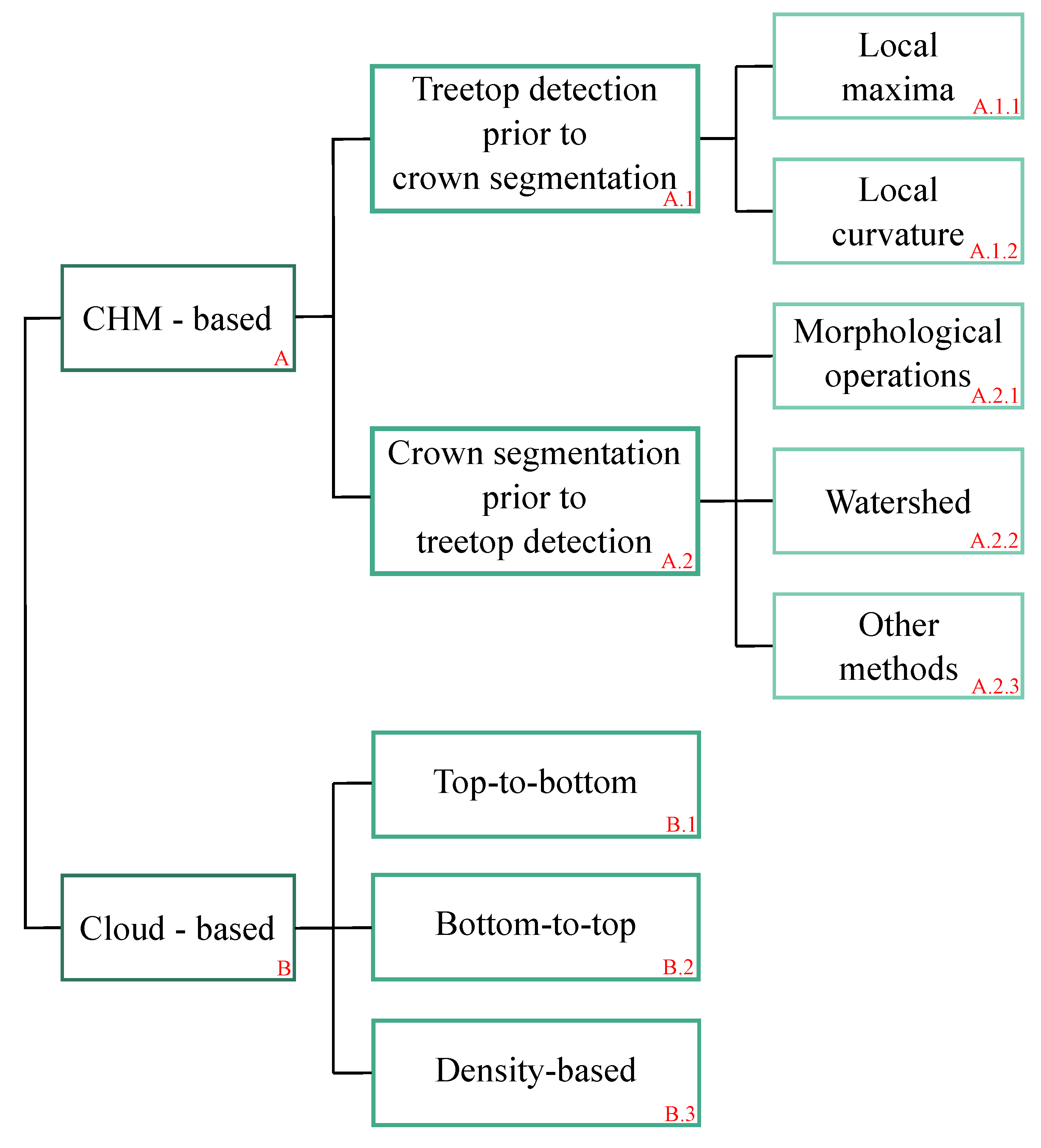
Figure 1. Classification of the methods that have been proposed so far to identify individual trees. The numbers in red correspond with the labels associated with the classification of the literature works shown in Table S1 of the Supplementary Material.
Remotesensing 13 00322 g001
Figure 2. Contextualization of the study site from the continental (a) to the national (b) and the local (c) scale; (c) location of the twelve study sites: the red, orange, and yellow colors indicate regular, random, and mixed (only a part is regular) tree patterns, respectively. (d) zoom over a natural tree stand, hereinafter called D 1 , and (e) a tree plantation, hereinafter called D 2 . (f) flight trajectories followed during the acquisition of LiDAR data over the Orco Valley, carried out on 28 February, 2019. Source: Google Earth.
Remotesensing 13 00322 g002
Figure 3. (a) lateral view of the point cloud representing an individual tree; (b) areal point density computed for the same tree after that all the point are projected on the ground (plane z = 0).
Remotesensing 13 00322 g003
Figure 4. Comparison between the performance of the local maxima (upper row) and the density-based (lower row) approaches when applied to (a) coniferous stands, and to deciduous tree stands in (b) leaf-on and (c) leaf-off conditions.
Remotesensing 13 00322 g004
Figure 5. Example of the algorithm’s output for D 1 . The resulting stems’ locations (red dots) can be imported in GIS and compared to field data (white dots).
Remotesensing 13 00322 g005
Figure 6. Conceptual representation of the individual tree identification algorithm.
Remotesensing 13 00322 g006
Figure 7. (a) count of the actual trees (# of trees) versus the count provided by the algorithm (# of detected trees) for the sites D 1 D 12 (red diamonds). The black line represents a perfect match. (b) accuracy metrics, where green, blue, and orange indicate recall, precision, and F-score metrics, respectively.
Remotesensing 13 00322 g007
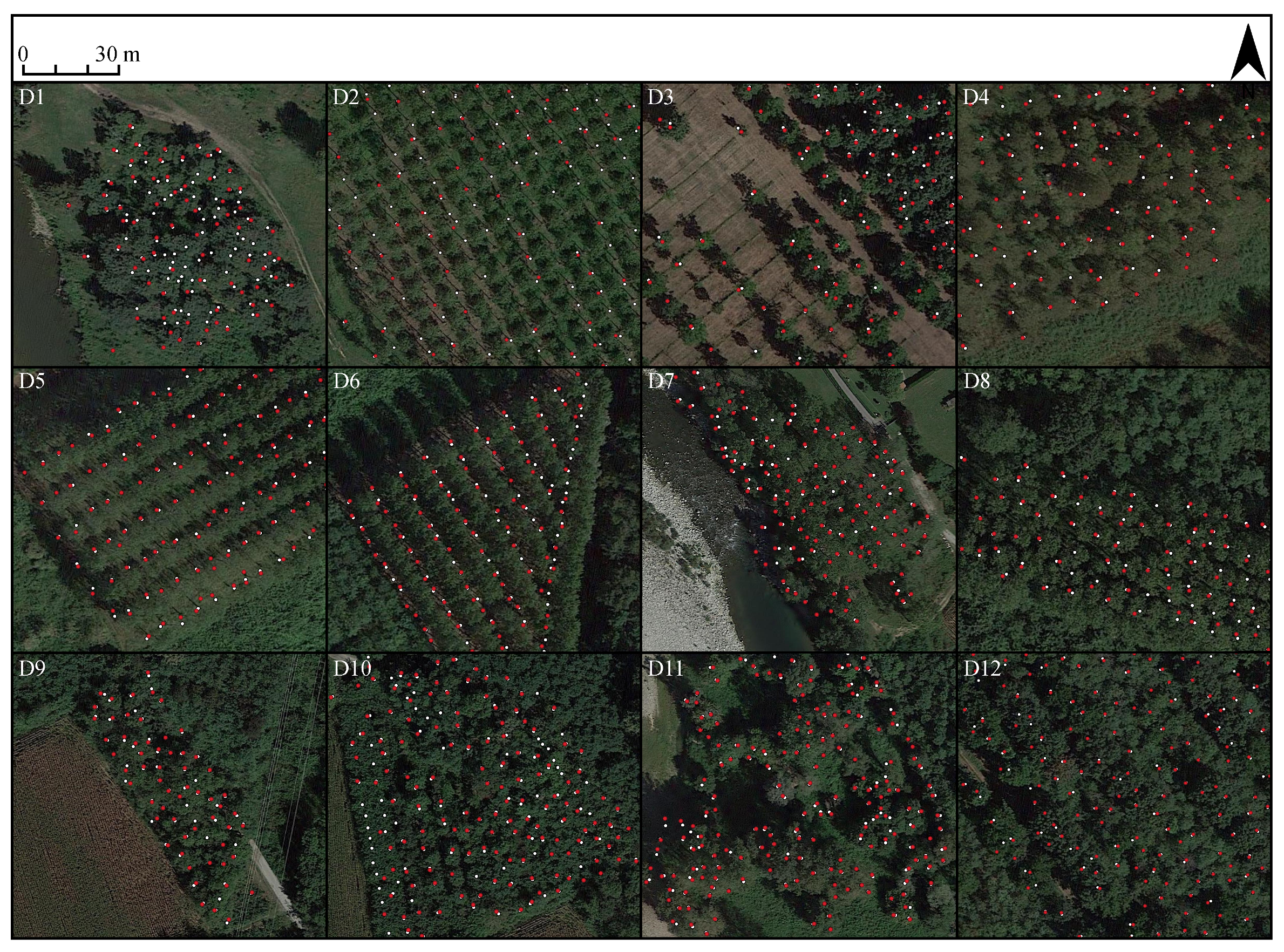
Figure 8. View of the twelve study areas from Google Earth. Red and white dots indicate the algorithm-derived and field measured stem locations, respectively.
Remotesensing 13 00322 g008
Figure 9. (a) Percentage reduction of the elapsed time for different clipping radii with respect to the case of infinite clipping radius. F-score for different values of the clipping radius parameter (b), and the critical length parameter (c).
Remotesensing 13 00322 g009
Figure 10. (a) Percentage time reduction, (b) F-score, and (c) position error at different re-sampling rates for considered twelve study areas.
Remotesensing 13 00322 g010
Table 1. Main features of the twelve study areas. The coordinates refer to the centroid of the area according to the reference system EPSG:25832. The tree count and information derive from the field survey carried out on February 2019.
Area IDCoordinatesTreeTreeTreePerimeterAreaPointNotes
PatternSpeciesAge(m)(ha)Density
D145 ° 14 22.27 N;randomPopulus spp.,mature2400.418.7 ± 4.4-
07 ° 48 45.10 E Robinia Ps.
D245 ° 19 01.73 N;regularPopulus spp.various6202.407.5 ± 4.2-
07 ° 44 16.98 E
D345 ° 12 06.02 N;mixedPopulus spp.young8344.398.7 ± 3.7-
07 ° 50 26.61 E
D445 ° 10 58.61 N;regularPopulus spp.various3320.685.8 ± 2.1a warehouse
07 ° 52 07.15 E 4 × 4 ×2 m
D545 ° 11 44.09 N;regularPopulus spp.mature3130.4010.2 ± 3.4-
07 ° 51 36.33 E
D645 ° 11 40.61 N;regularPopulus spp.mature3080.579.6 ± 3.6-
07 ° 51 38.04 E
D745 ° 20 02.58 N;randomPopulus spp.various3390.6213.5 ± 7.5fence
07 ° 44 01.05 E height: 2.5 m
D845 ° 12 25.45 N;regularPopulus spp.,mature3160.4117.8 ± 8.1-
07 ° 50 32.02 E Quercus spp.
D945 ° 18 06.05 N;randomRobinia Ps.mature2500.2710.1 ± 5.4power lines
07 ° 46 03.51 E
D1045 ° 18 08.24 N;mixedPopulus spp.,mature3570.818.2 ± 4.6-
07 ° 45 59.95 E Robinia Ps.
D1145 ° 12 34.08 NrandomPopulus spp.,mature4351.2011.9 ± 7.2-
07 ° 50 06.51 E Quercus spp.
D1245 ° 12 06.08 N;regularPopulus spp.mature5721.938.7 ± 3.8-
07 ° 50 26.58 E
Table 2. Comparison between the count of actual trees and the count of the trees detected by the algorithm, the accuracy metrics, the position error, and the main statistics of the stem-to-top distance for each study area.
Area ID# of Trees# of Detected TreesRecallPrecisionF-ScorePosition Error (m)Stem-to-Top Distance (m)
MinMaxMean
D198760.780.960.861.2502.120.79
D22841660.581.000.740.8002.080.63
D35436201.000.840.920.8102.060.62
D41021331.000.750.860.8601.670.65
D51321441.000.910.950.8201.790.53
D61511230.811.000.900.7401.350.54
D71301250.960.990.980.7801.700.66
D8109970.891.000.941.0001.310.60
D965600.921.000.960.9101.190.56
D101851470.790.990.780.9101.910.55
D112102101.001.001.000.7301.500.63
D123053171.000.930.970.8601.830.70
Table 3. Elapsed time and number of points of the input point cloud for each study area. In the reported cases, the clipping radius is equal to 20 m.
Area IDElapsed Time (s)Number of Points
D141.8719,510
D24.284500
D3195.0997,568
D436.5524,679
D511.429995
D617.4313,391
D7142.9345,617
D859.9129,935
D934.7515,860
D1055.0031,865
D11123.9158,808
D12413.62127,192
Table 4. Comparison between the measured, the optimal and the computed stem spacing.
Area IDReal Spacing (m)Optimal Spacing (m)Computed Spacing (m)
D12.52.02.8
D26.01.55.8
D33.03.02.5
D48.04.02.8
D55.03.52.8
D62.52.03.1
D73.53.53.3
D83.53.53.8
D94.04.04.1
D104.04.04.2
D113.03.03.1
D125.04.54.4
Table 5. Summary of the main advantages and limitations of the presented algorithm along with notes for its application.
AdvantagesLimitationsNotes
Low sensitivity to the tree spatial arrangement and the presence of understory vegetation.Better performance in homogenous stands.Splitting of datasets into homogenous areas before its application.
Working on the entire point clouds.Long computation time for high number of input points.In the case of large datasets, algorithm’s parallelization or dataset’s sub-sampling.
Requiring 2 points·m 2 as minimum point densityWorse performance if dealing with local data inaccuraciesData quality inspection before its application.
Good accuracy with the default parameter setting.Necessity of field calibration for the derived treetops height.Visual inspection of the study areas before its application.
Publisher’s Note: MDPI stays neutral with regard to jurisdictional claims in published maps and institutional affiliations.