High-Resolution SAR Image Classification Using Multi-Scale Deep Feature Fusion and Covariance Pooling Manifold Network

Abstract

The classification of high-resolution (HR) synthetic aperture radar (SAR) images is of great importance for SAR scene interpretation and application. However, the presence of intricate spatial structural patterns and complex statistical nature makes SAR image classification a challenging task, especially in the case of limited labeled SAR data. This paper proposes a novel HR SAR image classification method, using a multi-scale deep feature fusion network and covariance pooling manifold network (MFFN-CPMN). MFFN-CPMN combines the advantages of local spatial features and global statistical properties and considers the multi-feature information fusion of SAR images in representation learning. First, we propose a Gabor-filtering-based multi-scale feature fusion network (MFFN) to capture the spatial pattern and get the discriminative features of SAR images. The MFFN belongs to a deep convolutional neural network (CNN). To make full use of a large amount of unlabeled data, the weights of each layer of MFFN are optimized by unsupervised denoising dual-sparse encoder. Moreover, the feature fusion strategy in MFFN can effectively exploit the complementary information between different levels and different scales. Second, we utilize a covariance pooling manifold network to extract further the global second-order statistics of SAR images over the fusional feature maps. Finally, the obtained covariance descriptor is more distinct for various land covers. Experimental results on four HR SAR images demonstrate the effectiveness of the proposed method and achieve promising results over other related algorithms.

1. Introduction

Synthetic aperture radar (SAR) is an all-weather and all-day active microwave imaging system. Due to the special capabilities, the SAR system has become a very significant and powerful source of information for various fields, such as land-cover mapping, disaster monitoring, and urban planning [1]. Classifying and interpreting the information provided by SAR images is usually recognized as a prerequisite step among these applications. In recent years, the new generation of space- or airborne SAR sensors can acquire large amounts of high-resolution (HR) SAR images [2]. These data provide sufficient information in the spatial context for SAR scene understanding and interpretation. Nevertheless, HR SAR image classification still faces the following two challenges:

• Intricate spatial structural patterns: Due to the coherent imaging mechanism and object shadow occlusion, pixels of the same object will present a high degree of variability, known as speckle [3]. Moreover, HR SAR images contain more strong scattering points, and the arrangements of numerous and various objects have become more complicated. In this context, HR SAR images will have a great intra-class variation and little inter-class difference between objects [4]. As shown in Figure 1a,b, we have given two low-density residential areas from the same category and two different categories including open land and water areas. Therefore, extracting more discriminative and precise spatial features for HR SAR image classification is still a highly challenging task.
• Complex statistical nature: The unique statistical characteristics of SAR data are also crucial for SAR image modeling and classification. In HR SAR images, the number of elementary scatterers present in a single-resolution cell is reduced. Traditional statistical models for low- and medium-resolution SAR, such as Gamma [5], K [6], Log-normal [7], etc., find it difficult to provide a good approximation for the distribution of HR SAR data. Meanwhile, accurate modeling of HR SAR data using statistical models may require designing and solving more complex parameter estimation equations. Hence, it is also a challenge to effectively capture the statistical properties contained in the SAR image to enhance the discrimination of land-cover representations.

1.1. Related Work

The mainstream methods for SAR image classification can be roughly categorized as hand-crafted feature-based methods, statistical analysis-based methods, and deep learning methods. We briefly review these related works and then discuss the inspiration from these methods.

In recent years, many handcrafted feature descriptors have been proposed to characterize the content of SAR images, such as multilevel local pattern histogram (MLPH) feature [8], Ratio-detector-based feature [9], contextual descriptors [10], etc. These features exhibit better performance compared to GLCM [11] and Gabor features [12] in HR SAR image classification. In addition, Tombak et al. [13] investigated the use of the recently developed feature attribute profiles (FPs) for the feature extraction of SAR images. Song et al. [14] employed the histogram of oriented gradients (HOG)-like features to effectively capture the main structures of targets in speckled SAR images. Guan et al. [15] used the covariance descriptor of textural features and made the feature descriptor more distinguishable for various SAR land covers. Generally, the above features are fed into a classifier such as the Softmax [16] or the support vector machines (SVM) [17] for classification. To some extent, hand-crafted feature-based methods have excellent low-level feature representation capabilities of SAR images and can perform reasonably well for some specific categories with minimal amounts of training data. However, HR SAR images contain more complex structural and geometrical information, which requires hand-crafted feature-based methods needed to further improve robustness and generalization performance. Therefore, the more abstract and discriminative features need to be extracted from the above low-level features for complex HR SAR classification tasks.

Due to the unique characteristic of the coherent speckle, the distribution of pixel values within SAR images provides much valuable information. Statistically modeling the terrain distributions is an effective tool for SAR image analysis. There are already some traditional non-Gaussian models to describe the distribution characteristics of SAR images, such as Fisher [18], generalized Gamma [19], Nakagami-Gamma [20], heavy-tailed Rayleigh [21], etc. To fully capture the complex content of HR SAR images, some new statistical models, such as the scale mixture of Gaussian (SMoG) [22], generalized Gamma hybrid model [23], lognormal mixture model [24], beta generalized normal distribution [25], and complex generalized Gaussian model [26], have been proposed for statistical analysis. Frery et al. [27] propose a generalized statistical framework for HR SAR images. Generally, these models are then used in a Bayesian inference framework such as Markov random field [28] to realize classification. However, these statistical models generally have strict assumptions or are effective for specific scenarios. Meanwhile, parameter estimation is also very important for the accurate modeling of HR SAR data. Besides, these models are based on pixel values and do not establish effective relationships with high-level features. We find that the essence of the statistical model is to capture the high-order statistics of SAR images for data representation. Therefore, the above analysis inspires us to capture statistics from high-level features of SAR images that may be able to obtain more efficient and discriminant feature representations.

Deep neural networks (DNN) [29] are capable of learning high-level features of images hierarchically. Many studies have verified the powerful ability of DNN to discover significant features and semantic relationships in SAR image classification. Geng et al. [30,31] proposed a deep supervised and contractive neural network (DSCNN) for SAR feature learning. Zhao et al. [32] proposed a discriminant deep belief network (DisDBN) for HR SAR image classification. Ding et al. [33] investigated the capability of convolutional neural networks (CNN) combined with data augmentation operations in SAR target recognition. Chen et al. [34] proposed an all-convolutional network (A-CovNet) for SAR target recognition, which consists of only sparsely connected layers to prevent over-fitting problems. Li et al. [35] applied CNN to very-high-resolution SAR image classification. However, the above-mentioned learning methods require a large number of labeled data to obtain a satisfactory result. In actual application scenarios, manually annotating SAR data is labor-intensive and time-consuming. Considering the scarcity of SAR labeled data, many schemes such as domain adaptation [36], transfer learning [37], GAN [38], and unsupervised feature learning [39], etc., have been proposed to solve the SAR image classification problem. The sparse unsupervised feature learning has relatively simple structures and is a feasible solution to relieve the needs of labeled samples. Recently, a new unsupervised feature learning method [40] based on the dual-sparse encoder has been proposed. This method optimizes the cost function driven by natural rules and performs hierarchical unsupervised learning on CNN. However, [40] does not adequately consider the influence of coherent speckles from SAR images, and the complementarity of features between different levels is not fully utilized. Therefore, it is necessary to construct a CNN model for extracting high-level features from HR SAR images. This model can make full use of a large number of unlabeled data for feature learning and can take into account the complementarity of features between different levels, to realize the discriminant feature extraction of SAR objects.

1.2. Motivations and Contributions

Based on an overall consideration, the objective of this paper aims at combining the advantages of statistical analysis and representation learning to realize pixel-based classification of HR SAR images with resolution equal to or even less than 1 m. First, some previous CNN models [34,35] only use the features of the last convolutional layer for SAR image classification without the full consideration of the information obtained by the additional layers. Second, to capture statistics from high-level features of SAR images, Liu et al. [41] proposed a statistical CNN (SCNN) for land-cover classification from SAR images, which characterize the distributions of CNN features by the first- and second-order statistics (including mean and variance). However, the variance only considers the statistical properties of independent feature maps and does not establish the interaction between the feature maps. As a second-order statistical method, covariance has a more robust representation than the mean and variance [42]. He et al. [43] proposed a method that combines multi-layer CNN feature maps and covariance pooling for optical remote sensing scene classification. Ni et al. [44] proposed a multimodal bilinear fusion network, which used the covariance matrix to fuse the optical and SAR features for land cover classification. Generally, the above methods map the covariance directly to the Euclidean space through the matrix logarithm operation for classification [45]. However, they do not further extend the covariance matrix to the deep network to deeply mine the potential discriminant features of second-order statistics.

To tackle the above problems, we propose a novel HR SAR image classification method, using a multi-scale deep feature fusion network and covariance pooling manifold network (MFFN-CPMN). MFFN-CPMN combines the advantages of local spatial features and global statistical properties and considers the multi-feature information fusion in representation learning to describe a SAR image. To our knowledge, this is the first approach that integrates the CPMN with the CNN for classification HR SAR images with a resolution equal to or even less than 1 m. The main contributions of this paper lie in two folds.

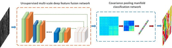
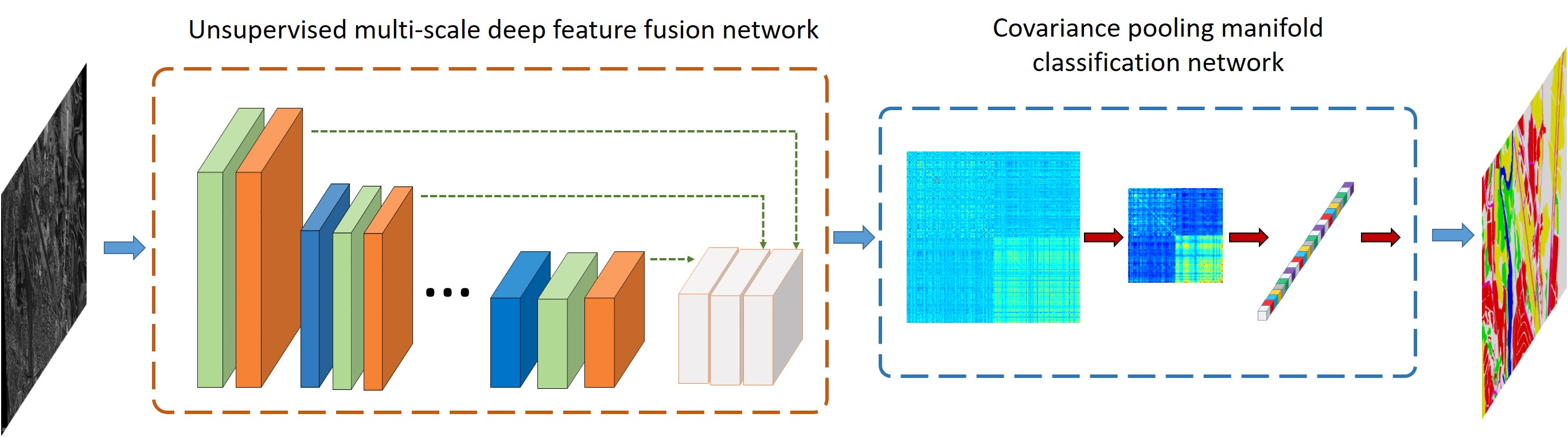
• We propose a Gabor-filtering-based multi-scale feature fusion network (MFFN) to obtain the effective spatial feature representation. MFFN combines the strengths of unsupervised denoising dual-sparse encoder and multi-scale CNN to learn discriminative features of HR SAR images. Meanwhile, MFFN introduces the feature fusion strategies in both intra-layer and inter-layer to adequately utilize the complementary information between different layers and different scales.
• We introduce a covariance pooling manifold network (CPMN) to capture the statistical properties of the HR SAR image in the MFFN feature space. The CPMN characterizes the distributions of spatial features by covariance-based second-order statistics and incorporates the covariance matrix into the deep network architecture to further make the global covariance statistical descriptor more discriminative of various land covers.

The rest of this paper is organized as follows. The proposed classification method MFFN-CPMN is described in Section 2. Experimental results and analysis on three real HR SAR image data are presented in Section 3. Finally, the conclusion is drawn in Section 4.

2. Materials and Methods

Figure 2 shows the schematic of the proposed MFFN-CPMN-based classification method for the HR SAR image. In general, the proposed method consists of the following two steps: (1) Gabor filtering-based multi-scale deep fusion feature extraction; (2) global second-order statistics extraction and classification based on covariance pooling manifold network. The proposed method is elaborated in detail in the following subsections.

2.1. Gabor Filtering-Based Multi-Scale Deep Fusion Feature Extraction

2.1.1. Extraction of Gabor Features

CNN can learn the high-level representation from the low-level features of the SAR data in a hierarchical way. Thus, the representation ability of the low-level features will affect the following high-level representation. The backscattering of the single-polarized HR SAR image is very sensitive to the shape and orientation of the scatterers. Moreover, complex geometrical information and coherent speckle exist in the SAR image. If only the raw image is used to optimize the first layer parameters of the network, the above factors may harm the performance of CNN in extracting SAR image features. Taking into account that the Gabor filter [46] has direction selection characteristics, it is compatible with the orientation-sensitive of the SAR image. Gabor filtering can extract rich multi-scale and multi-direction spatial information, which may reduce the feature extraction burden of CNN.

The Gabor filter is modulated by a Gaussian function and a sinusoidal plane wave [47], whose general function can be defined as:

$$\begin{array}{l}{\mathrm{G}}_{u,v}(x,y)=\frac{f^2}{\pi \gamma \eta }\exp \left(-\left({\alpha }^2{x^{\prime }}^2+{\beta }^2{y^{\prime }}^2\right)\right)\exp \left(j2\pi f{x}^{\prime }\right)\\ x^{\prime }=x\cos \theta +y\sin \theta , y^{\prime }=-x\sin \theta +y\cos \theta \end{array}$$

(1)

where $f$ is the central frequency of the sinusoid. $\theta$ denotes the orientation of the Gabor function. $\alpha$ and $\beta$ is the sharpness of the Gaussian along the two axes, respectively. $\gamma =f/\alpha$ and $\eta =f/\beta$ are defined to keep the ratio between frequency and sharpness.

To get Gabor features, a set of Gabor filters with different frequencies and orientations are required as follows:

$$f={f_{\max }/\sqrt{2}}^u,{\theta }_v=\frac{v}{8}\pi u=0,\dots ,U-1,v=0,\dots ,V-1.$$

(2)

Here, $f_{\max }$ is the highest peak frequency of the Gabor function. $U$ and $V$ represents the number of scales and orientations of Gabor filters, respectively. Then, Gabor features are extracted by convoluting the SAR image $\mathrm{I}(x,y)$ with every Gabor filter ${\mathrm{G}}_{u,v}(x,y)$ as follows:

$${\mathrm{F}}_{u,v}(x,y)=\left|\mathrm{I}(x,y)\otimes {\mathrm{G}}_{u,v}(x,y)\right|,$$

(3)

where ${\mathrm{F}}_{u,v}$ denotes the Gabor features corresponding to scale $v$ and orientation $u$, respectively. $\otimes$ and $|\cdot |$ are convolution and absolute operators, respectively. By stacking the Gabor feature maps with different scales and different orientations, this step can enrich the low-level features of objects used for CNN classification.

2.1.2. Multi-Scale Deep Feature Fusion Network

The main three components of the traditional CNN are a convolutional layer, a nonlinear activation layer, and a pooling layer. Formally, the forward pass operations of the $l\mathrm{th}$ layer in CNN can be defined as follows:

$${\mathrm{F}}^l=pool\left(\sigma \left({\mathrm{F}}^{l-1}\otimes {\mathrm{W}}^l+{\mathrm{b}}^l\right)\right),$$

(4)

where ${\mathrm{F}}^{l-1}$ is the input feature map of the $l\mathrm{th}$ layer, ${\mathrm{W}}^l$ and ${\mathrm{b}}^l$ are weights and bias of the $l\mathrm{th}$ layer, respectively. $\sigma (\cdot )$ is the nonlinear activation function, and the sigmoid function is used in our work. $pool(\cdot )$ denotes the pooling operation. The input features ${\mathrm{F}}^0$ of the first layer of CNN are the Gabor features extracted above.

HR SAR images contain both complex objects and extended areas. On the one hand, the traditional CNN using a single-scale convolution kernel may not accurately capture local details of different sizes. On the other hand, our CNN model is trained in a greedy layer-wise unsupervised learning manner. The complementarity of features between different layers cannot be captured due to the lack of feedback information. Moreover, the shallow features of CNN tend to extract the local spatial structural information, while the deep features contain the global spatial layout information of the objects. Based on the above analysis, we need to excavate the potential information hidden in different scales and different layers to improve the feature representation capacity. Thus, we present two fusion strategies in our multi-scale feature fusion network (MFFN) to integrate local and global features between different scales and layers.

The first one is intra-layer fusion, which emphasizes the fusion of various local information in each layer. Specifically, inspired by the inception module [48], we aim to capture the multi-scale information from the input features of each layer. As shown in Figure 3a, an original inception model is given. It used multiple convolutional layers with different kernel sizes to extract the multi-scale feature. The output features are further concatenated as the final output. In our experiment, we find that the $1\times 1$ convolution kernel does not bring meaningful improvement to the accuracy. This may be because the $1\times 1$ convolution focuses on the location itself and cannot obtain enough neighbor information. Thus, as shown in Figure 3b, we propose to construct a multi-scale convolution module by using filters of sizes 3, 5, and 7. In addition, since the unsupervised learning method we adopted allows the model with large numbers of input feature channels efficiently, the feature concatenation will significantly increase the model parameter amount and computational burden. Considering a balance between accuracy and computational cost, we adopt the sum-based fusing mechanism to reduce feature dimensions and improve efficiency. The accuracy and computational cost are reported in the experiments. Correspondingly, the process of intra-layer fusion can be expressed as follow:

$${\mathrm{F}}_{sum}^l=pool\left(\sigma \left({\mathrm{F}}_{s=3}^l\right)+\sigma \left({\mathrm{F}}_{s=5}^l\right)+\sigma \left({\mathrm{F}}_{s=7}^l\right)\right),$$

(5)

where ${\mathrm{F}}_{sum}^l$ represents the fused features of the $l\mathrm{th}$ layer, $s$ denotes the convolution kernel size at the current scale. ${\mathrm{F}}_s^l$ represents the convolution feature output of the filter of size $s$. Figure 2 shows the visualized multi-scale convolution feature maps. It can be seen that by introducing different kinds of convolution kernels, the diversity of extracted local features are increased. These features are conducive to further improving the feature representation ability of our model.

The second strategy is inter-layer fusion. As we know, the features of different layers contain different levels of spatial-contextual information. The shallow features mine low-level structure information, while the deep layers generate the high-level semantical features. To compensate for the loss of interaction information between layers due to the unsupervised layer-wise training, we fuse the features from different layers to capture the complementary information and enhance global feature representation. As shown in the green dashed line in Figure 2, the features of each layer in MFFN are concatenated to obtain the final fusional features. We do not use summation fusion here because summation fusion is difficult to retain the special information of the features of each layer, which may cause the information loss of the local structure. Besides, since the spatial dimension of different layers is inconsistent, we adopt the average pooling operation to transform the dimensions of all layers to be consistent. Finally, the feature fusion can be easily performed with a way of concatenation. The whole process can be represented by the following equations:

$${\mathrm{F}}_{fusion}=g_1\left({\mathrm{F}}_{sum}^1\right)\cup \cdot \cdot \cdot \cup g_l\left({\mathrm{F}}_{sum}^l\right)\cup \cdot \cdot \cdot \cup g_L\left({\mathrm{F}}_{sum}^L\right),$$

(6)

where ${\mathrm{F}}_{sum}^l$ is the output feature maps of the $l\mathrm{th}$ layer, the $g_l$ denotes the dimension-matching function based on average pooling. $\cup$ refers to the concatenation operation. ${\mathrm{F}}_{fusion}$ denotes the final fusional features of MFFN. To illustrate the effect of our fusion strategy, the different ways of fusing features are also verified in the experiments.

In the orange part of Figure 2, a two-layer MFFN model is presented. First, the whole model takes Gabor features as input and obtains multi-scale feature maps through multi-scale convolution. Then, the nonlinear activation and summation fusion of the features are carried out. The final multi-scale fusional feature output is obtained by concatenation of multi-layer features. Note that our pooling step uses a $3\times 3$ pooling region size with $\mathrm{pad}=2$ instead of a $2\times 2$ pooling size to reduce the grid effect. This is mainly because the $2\times 2$ pooling regions are disjointed, and more information is lost in each pooling layer. The overlapping pooling can reduce the spatial information loss of each layer to a certain extent, thereby improving the performance of the model [49].

2.1.3. Greedy Layer-Wise Unsupervised Feature Learning

An important aspect is how to train the weights $\mathrm{W}$ and bias $\mathrm{b}$ of the proposed MFFN model. Considering the limited SAR labeled samples, we update the parameters of MFFN by the layer-wise pre-training based on the unsupervised criterion [50]. Benefitting from the characteristics of meta parameters-free and simple rules, we introduce a new denoising dual-sparse encoder to realize the unsupervised learning of model parameters. The blue box of the first part in Figure 2 shows the proposed denoising dual-sparse encoder. Next, the detailed denoising dual-sparse encoder algorithm is described. To train the parameters of the $l\mathrm{th}$ layer, a set of small unlabeled patches ${\mathrm{D}}_s^{l-1}\in R^{N\times P}$ randomly extracted from the output feature maps of the $(l-1)\mathrm{th}$ layer as the training data. $N$ is the number of patches. Every row of ${\mathrm{D}}_s^{l-1}$ is a vectorized patch and $P=s^2\cdot N_h^{l-1}$ is the dimension of vectorization. $N_h^{l-1}$ is the output dimension of $(l-1)\mathrm{th}$ layer. Then, inspired by the denoising autoencoder [51], we applied the denoising mechanism to the dual-sparse encoder model. We found that introducing this operation can further enhance the robustness of the model to noise. Specifically, we corrupt ${\mathrm{D}}_s^{l-1}$ into the vector ${\stackrel{\sim }{\mathrm{D}}}_s^{l-1}$ with a certain probability $\lambda$ through a stochastic mapping:

$${\stackrel{\sim }{\mathrm{D}}}_s^{l-1}\sim \phi \left({\stackrel{\sim }{\mathrm{D}}}_s^{l-1}|{\mathrm{D}}_s^{l-1},\lambda \right),$$

(7)

where $\phi \left(·\right)$ is a type of distribution determined by the original distribution of ${\mathrm{D}}_s^{l-1}$ and the type of random noise added to ${\mathrm{D}}_s^{l-1}$. In general, $\phi$ is set to Bernoulli distributions, and the element components in the input ${\mathrm{D}}_s^{l-1}$ are randomly forced to 0 with the probability of $\lambda$ ($\lambda$ is set to 0.5 in our work), and the others are left untouched.

For the $l\mathrm{th}$ layer, the feature output formula is as follows:

$${\mathrm{H}}_s^l=\sigma \left({\stackrel{\sim }{\mathrm{D}}}_s^{l-1}{\mathrm{W}}_s^l+{\mathrm{b}}_s^l\right),$$

(8)

where ${\mathrm{H}}_s^l\in R^{N\times N_{{}_h}^l}$ is the feature output matrix of the $l\mathrm{th}$ layer. ${\mathrm{W}}_s^l\in R^{P\times N_h^l}$ and ${\mathrm{b}}_s^l\in R^{1\times N_{{}_h}^l}$ are the weights and bias at the $s$ scale of the $l\mathrm{th}$ layer convolution kernel, respectively. Notably, the ${\mathrm{W}}_s^l$ here corresponds to the convolution kernel of each scale under each layer in MFFN. Thus, the trained parameter ${\mathrm{W}}_s^l$ can be reshaped into the form ${\mathrm{W}}_s^l\in R^{s\times s\times N_h^{l-1}\times N_h^l}$, and are applied to the location of the corresponding convolution kernel. To form a sparse optimization function, a dual sparse encoder based on enforcing population and lifetime sparsity (EPLS) [40] is used to restricts the ${\mathrm{H}}_s^l$ units to have a strong dual sparsity and builds a one-hot sparse target matrix ${\mathrm{T}}_s^l$. Finally, the parameters can be upgraded by minimizing the L2 norm of the difference between ${\mathrm{H}}_s^l$ and ${\mathrm{T}}_s^l$:

$${\mathrm{W}}_s^{l\ast },{\mathrm{b}}_s^{l\ast }=\arg \underset{{\mathrm{W}}_s^l{,\mathrm{b}}_s^l}{\min }{\displaystyle \sum _s^S{\Vert {\mathrm{H}}_s^l-{\mathrm{T}}_s^l\Vert }_2^2},$$

(9)

The model can be efficiently trained through the mini-batch stochastic gradient descent with adadelta [52] adaptive learning rate. Figure 4 shows the model structure of the denoising dual-sparse encoder. After the model completed the training of the current layer, the weights are applied to the convolution kernel location to obtain the output convolution feature map as the input of the next layer. Repeat the training process until the parameters of all layers are pre-trained. The whole procedure of optimizing parameters is purely unsupervised, and there is no need to carry out the fine-tuning after the layer-wise training.

We can summarize our MFFN feature extraction in detail in Algorithm 1. The superiority of the proposed MFFN method is threefold. First, the Gabor filtering can enhance the richness of low-level features and reduce the training burden of the MFFN. Second, the multi-scale convolution module based on unsupervised learning can enrich the diversity of features in intra-layer and make full use of a large number of unlabeled patches as training data. Last but not least, the two different fusion strategies are adopted in both intra-layer and inter-layer, which can not only strengthen various local information in different scales but also capture complementary and interaction information between different layers. The three advantages mentioned above enable the MFFN that becomes a very effective feature extraction model for HR SAR data under a relatively shallow network structure.

Algorithm 1 Gabor filtering-based multiscale unsupervised deep fusion feature extraction.

Input: The SAR image $\mathrm{I}$, Layer number $\mathrm{L}$

1: Extract Gabor features of the SAR image based on (1).

2: Initialize input feature maps ${\mathrm{F}}^0=\left\{{\mathrm{F}}_{u,v},u=0,\dots ,U-1,v=0,\dots ,V-1\right\}$;

3: Initialize weights and bias $\mathrm{W},\mathrm{b}\sim {\rm N}\left(0,0.01\right)$;

4: for $l=1$ to $\mathrm{L}$ do

5:  Generate ${\mathrm{D}}_s^{l-1},s=3,5,7$ by randomly extracting $N$ patches from ${\mathrm{F}}_{sum}^{l-1}$; Corrupt ${\mathrm{D}}_s^{l-1}$

into ${\stackrel{\sim }{\mathrm{D}}}_s^{l-1}$, and map ${\stackrel{\sim }{\mathrm{D}}}_s^{l-1}$ to ${\mathrm{H}}_s^l$ by (7) and (8);

6:  Obtain ${\mathrm{W}}_s^{l-1}$, ${\mathrm{b}}_s^{l-1}$ by solving (9) and update the parameters of MFFN;

7:  Extract $l\mathrm{th}$ layer multiscale feature ${\mathrm{F}}_s^l$ of MFFN by (2), and get the final feature output

by sum fusion: ${\mathrm{F}}_{sum}^l=pool\left(\sigma \left({\mathrm{F}}_{s=3}^l\right)+\sigma \left({\mathrm{F}}_{s=5}^l\right)+\sigma \left({\mathrm{F}}_{s=7}^l\right)\right)$;

8: end for

Output: The pretrained MFFN model.

2.2. Global Second-Order Statistics Extraction and Classification Based on CPMN

During the feature classification stage, mainstream CNNs typically use global average pooling [53] to aggregate the output features at the end of the network. However, this method can only capture the first-order information of features, thereby ignoring the statistical properties of a SAR image between feature channels. It makes the model less adaptable to complex tasks such as SAR image classification. To make the feature representation more powerful, we adopt a second-order statistical method based on covariance analysis to extract more discriminatory and valuable features.

2.2.1. Multilayer Feature Fusion Based on Covariance Pooling

To construct the input of CPMN, covariance pooling is used to form a covariance matrix for the output features of MFFN. Following the process in Figure 1, we take an $64\times 64$ input sample as an example, and the number of features is set to $N_h$. We have the feature output ${\mathrm{F}}_{\mathrm{sum}}^1\in R^{64\times 64\times N_h}$ of the first layer and the feature output ${\mathrm{F}}_{\mathrm{sum}}^2\in R^{32\times 32\times N_h}$ of the second layer. Then, we average pooling the feature ${\mathrm{F}}_{\mathrm{sum}}^1$ to obtain the downsampling feature ${\widehat{\mathrm{F}}}_{\mathrm{sum}}^1\in R^{32\times 32\times N_h}$, making it consistent with the spatial dimension of the second layer of features ${\mathrm{F}}_{\mathrm{sum}}^2$. After that, we stack the features of each layer to get the fusional features ${\mathrm{F}}_{fusion}=\left[{\widehat{\mathrm{F}}}_{\mathrm{sum}}^1;{\mathrm{F}}_{\mathrm{sum}}^2\right]\in R^{32\times 32\times 2N_h}$. Finally, the covariance matrix can be computed as:

$$\mathrm{C}=\frac{1}{n-1}{\displaystyle \sum _{j=1}^n\left(f_j-\mu \right)}{\left(f_j-\mu \right)}^T,$$

(10)

where $f_j,j=1,\dots ,n$ detnotes vectorization of ${\mathrm{F}}_{fusion}$ along the third dimension and $\mu =\left(1/n\right){\displaystyle {\sum }_{j=1}^n{f}_j}$. To make the covariance matrix strictly positive definite (SPD), regularization [44] is applied to $\mathrm{C}$. The covariance matrix by adding a multiple of the trace to diagonal entries of the covariance matrix:

$${\mathrm{C}}^{+}=\mathrm{C}+\epsilon \cdot trace\left(\mathrm{C}\right)\tilde{\mathrm{I}},$$

(11)

where $\epsilon$ is a regularization value and $\tilde{\mathrm{I}}$ is the identity matrix. Compared with first-order statistical features, the covariance matrix brings second-order statistics, which can obtain better regional feature description ability.

2.2.2. Covariance Features Classification Based on Manifold Network

The covariance matrix obtained above usually resides on the Riemannian manifold of the SPD matrix [45]. The standard method is often to apply a logarithmic transformation to map the Riemannian manifold structure to the Euclidean space [43,54]. Then, the upper triangular matrix is vectorized and input into a linear classifier to achieve classification. However, the covariance matrix obtained by the multi-layer feature fusion of CNN has large dimensions. In [43], a channel-average fusion strategy is proposed to reduce the dimensionality of CNN feature maps. Nevertheless, we find that when applied to SAR image classification, the channel-average fusion may cause a significant informative loss of some channel features, thereby degrading the performance of covariance features. To obtain more discriminative covariance features, a Riemannian manifold network is adopted to achieve the covariance-based feature classification. This network not only integrates the covariance matrix into the deep network but also reduces the dimensionality of the covariance matrix without losing geometric structure. The main three building blocks of a manifold network [55] are bilinear mapping (BiMap) layers, eigenvalue rectification (ReEig) layers, and an eigenvalue logarithm (LogEig) layer, respectively. The light blue part in Figure 1 shows our manifold network classification framework.

Specifically, given a covariance matrix $\mathrm{C}$ as input, the BiMap layer transforms the input SPD matrices to new SPD matrices by a bilinear mapping $f_b$ as:

$${\mathrm{C}}_k=f_b\left({\mathrm{C}}_{k-1};{\mathrm{W}}_l\right)={\mathrm{W}}_k{\mathrm{C}}_{k-1}{\mathrm{W}}_k{}^T,$$

(12)

where ${\mathrm{C}}_{k-1}$ is the input SPD matrix of the $k\mathrm{th}$ layer. ${\mathrm{W}}_k\in {ℝ}^{d_k\times d_{k-1}}$ be weight matrix in the space of full rank matrices, ${\mathrm{C}}_k\in {ℝ}^{d_k\times d_k}$ is the resulting matrix. According to the manifold learning theory, retaining the original data structure is beneficial for classification. Thus, the BiMap layer reduces the dimensionality of the covariance matrix while preserving the geometric structure.

Then, a non-linearity is introduced by the ReEig layer to improve discriminative performance. The ReEig Layer is used to rectify the SPD matrix by tuning up their small positive eigenvalues:

$${\mathrm{C}}_k=f_r\left({\mathrm{C}}_{k-1}\right)={\mathrm{U}}_{k-1}\max \left(\tau \tilde{\mathrm{I}},{\sum }_{k-1}\right){\mathrm{U}}_{k-1}{}^T,$$

(13)

where ${\mathrm{U}}_{k-1}$ and ${\sum }_{k-1}$ are achieved by eigenvalue decomposition (EIG) ${\mathrm{C}}_{k-1}={\mathrm{U}}_{k-1}{\sum }_{k-1}{\mathrm{U}}_{k-1}{}^T$, $\tau$ is a rectification threshold. The max operation is element-wise matrix operation.

Further, to enable the covariance features to be classified on a standard Euclidean space classifier, we use the LogEig layer to map the output SPD matrices lie on the Riemannian manifold to the Euclidean space. Formally, the LogEig layer applied in $l\mathrm{th}$ layer is defined as:

$${\mathrm{C}}_k=\log \left({\mathrm{C}}_{k-1}\right)={\mathrm{U}}_{k-1}\log \left({\sum }_{k-1}\right){\mathrm{U}}_{k-1}{}^T,$$

(14)

where ${\mathrm{C}}_{k-1}={\mathrm{U}}_{k-1}{\sum }_{k-1}{\mathrm{U}}_{k-1}{}^T$ is an eigenvalue decomposition and log is an element-wise matrix operation.

In the end, the vector forms of the outputs can be fed into classical softmax layers for classification. The class conditional probability distribution of each sample the cross-entropy [56] is used to measure the prediction loss $L$ of the network based on

$$p_i^c=\frac{e^{z_i}}{{\displaystyle {\sum }_{t=1}^T{e}^{z_i}}},c=1,\dots ,T,L=-{\displaystyle \sum _c{c}_i\log \left(p_i\right)},$$

(15)

where $z_i$ is the vectorized feature vector of the LogEig layer, $T$ is the total number of classes. The matrix back-propagation methodology formulated in [55] is adopted to compute the partial derivative to the covariance matrix. The stochastic gradient descent is utilized to learn the network parameters. The implementation detail of optimizing the manifold network is summarized in Algorithm 2.

Algorithm 2 Manifold Network Training.

Input: Training samples $X=\left\{X_1,X_2,\dots ,X_M\right\}$, and corresponding labels $Y=\left\{Y_1,Y_2,\dots ,Y_M\right\}$, number

of BP epochs R.

1: compute covariance matrix $\mathrm{C}$ of each $X_m$ using (10) and (11);

2: Initialize weights $W_l$ of each BiMap layers, rectification $\tau =0.0001$;

3: while epoch $r=1$ to $R$ do

4:  while training sample $i=1$ to $M$ do

Compute the matrix mapping ${\mathrm{C}}_l$ by (12), (13) and (14);

Compute the softmax activation and the loss function by (15);

5:     Back-propagate error to compute cross-entropy loss gradient $\frac{\partial L}{\partial z_i}$;

6:     The loss of the k-th layer could be denoted by a function as $L^{(k)}=L\circ f^{(k-1)}\dots \circ f^{(1)}$

7:     Update network parameter of each layer based on partial derivatives

$\frac{\partial L^{{}^{(k)}}}{\partial W_k}=\frac{\partial L^{{}^{(k+1)}}}{\partial X_k}\frac{\partial f^{{}^{(k)}}}{\partial W_k}$, $\frac{\partial L^{{}^{(k)}}}{\partial X_{k-1}}=\frac{\partial L^{{}^{(k+1)}}}{\partial X_k}\frac{\partial f^{{}^{(k)}}}{\partial X_k}$

8:     The update formula for the BiMap layer parameter $W_l$ is

$W_k^{r+1}=\Gamma \left(W_k^r-\alpha \stackrel{\sim }{\nabla }{L}_{W_k^r}^{(k)}\right)$

where $\stackrel{\sim }{\nabla }{L}_{W_k^r}^{(k)}=\nabla L_{W_k^r}^{(k)}-\stackrel{\sim }{\nabla }{L}_{W_k^r}^{(k)}{\left(W_k^t\right)}^T{W}_k^t$, $\nabla L_{W_k^r}^{(k)}=2\frac{\partial L^{{}^{(k+1)}}}{\partial X_k}{W}_k^r{X}_{k-1}$;

9:     The gradients of the involved data in the layers below can be compute

$\frac{\partial L^{{}^{(k)}}}{\partial X_{k-1}}=2U\left(P^T\circ {\left(U^T\frac{\partial L^{{}^{(k^{\prime })}}}{\partial U}\right)}_{sym}\right)U^T+U{\left(\frac{\partial L^{{}^{(k^{\prime })}}}{\partial \sum }\right)}_{diag}{U}^T$

For the ReEig layers

$\frac{\partial L^{{}^{(k^{\prime })}}}{\partial U}=2{\left(\frac{\partial L^{{}^{(k+1)}}}{\partial X_k}\right)}_{sym}U\max (\tau I,\sum )$

$\frac{\partial L^{{}^{(k^{\prime })}}}{\partial \sum }=Q{U}^T{\left(\frac{\partial L^{{}^{(k+1)}}}{\partial X_k}\right)}_{sym}U$, $Q\left(i,i\right)=\left\{\begin{array}{c}1,\\ 0\end{array}\right.\begin{array}{c}\sum \left(i,i\right)>\tau \\ \sum \left(i,i\right)\le \tau \end{array}$

For the LogEig layer

$\frac{\partial L^{{}^{(k^{\prime })}}}{\partial U}=2{\left(\frac{\partial L^{{}^{(k+1)}}}{\partial X_k}\right)}_{sym}U\log \left(\sum \right)$, $\frac{\partial L^{{}^{(k^{\prime })}}}{\partial \Sigma }={\sum }^{-1}{U}^T{\left(\frac{\partial L^{{}^{(k+1)}}}{\partial X_k}\right)}_{sym}U$

10:     end while

11: end while

Output: The trained Manifold network classification model.

3. Results

3.1. Experimental Data and Settings

To validate the performance of the proposed method, four real HR SAR images obtained from different sensors, including the TerraSAR-X satellite, Gaofen-3 SAR satellite, China airborne SAR satellite, and F-SAR satellite were adopted. The detailed information of four real HR SAR images is shown in

Table 1. Detailed information on real HR SAR images.

Satellite	Band	Size	Resolution	Polarization	Date	Location
TerraSAR-X	X	1450*2760	0.5 m	HH	10/2013	Lillestroem, Norway
Chinese Gaofen-3	C	2600*4500	1 m	HH	03/2017	Guangdong, China
Chinese Airborne	Ku	1800*3000	0.3 m	HH	10/2016	Shaanxi, China
F-SAR	X	6187*4278	0.67 m	VV	10/2007	Traunstein, Germany

. For each dataset, the ground truth images are generated by manual annotation according to the associated optical image, which can be found in Google Earth.

TerraSAR-X data: The data of TerraSAR-X (http://www.intelligenceairbusds.com) are the region of Lillestroem, Norway. It was acquired in October 2013 with X-band and HH polarization. The image has $1450\times 2760$ pixels in size, and the resolution of this data is 0.5 m. The acquisition mode of the data is staring spotlight. The original image and the ground-truth are shown in Figure 5a,b. Five classes of interest are considered: Water, residential, roads, woodland, and open land.

Gaofen-3 data: The images of Gaofen-3 SAR records the area of Guangdong province, China, with C-band and HH polarization, which were acquired in March 2017. The size of this single-look data is $2600\times 4500$ with a spatial resolution of 1 m. The imaging mode is the sliding spotlight. The original image and the ground-truth are presented in Figure 6a,b. Six classes are included: Mountains, water, building, roads, woodland, and open land.

Airborne data: The third group of data is obtained from Chinese airborne covering the area of Shaanxi province, China, with Ku-band. The image is HH-polarization data with spotlight mode. The data were provided by the China Electronics Technology Group Corporation (CETC) Institute. The pixel size of this image size is $1800\times 3000$ pixels, and the spatial resolution is 0.3 m. Seven categories are included, which are open land, roads, rivers, runway, woodland, residential, and commercial. The original image and the ground-truth image are shown in Figure 7a,b.

F-SAR data: The fourth HR SAR image was acquired in Bavaria, Germany (https://www.dlr.de) with a VV-polar imaging mode. The data source is provided by an X-band F-SAR sensor of the German Aerospace Center. The image size is $6187\times 4278$, with a spatial resolution of 0.67 m. The original image and the ground-truth are shown in Figure 8a,b. Four typical categories are included: Water, residential, vegetation, and open land.

To achieve pixel-based classification, training, validation, and test samples are needed to be constructed. In our experiment, all the labeled pixels together with their neighborhood image patches are extracted to form the samples. $64\times 64$-pixel image patches were randomly selected according to the ground truth, which shows a balance between the classification accuracy and computational cost. Five hundred samples of each class were randomly selected and divided into training and validation, accounting for 90% and 10%. The other labeled pixels were used for the testing. In the testing phase, we used a stride greater than 1 to inference the test samples to avoid excessive computational costs. (we set the stride to 5 in our paper). The obtained class probability map then upsampled the original resolution with a negligible loss in the accuracy.

The overall accuracy (OA), average accuracy (AA), the kappa coefficient, and class-specific accuracy were used to measure the classification performance of the proposed method quantitatively. The optimal parameters of all methods were selected based on the best performance on the validation data. All results below were the mean values and standard deviations by running five times of the experiments. Furthermore, all experiments were implemented in MATLAB2014, with Intel I7 3.2-GHz CPU and 32-GB memory.

3.2. Parameter Settings and Performance Analysis of the Proposed MFFN-CPMN model

In this section, we first measured the sensitivity of different parameter settings on the classification results and determined the optimal parameters for the proposed method. As a public parameter choice, the Gabor filters were set with five scales and eight orientations, which include [0, (π/8), (π/4), (3π/8), (π/2), (5π/8), (3π/4), (7π/8)]. This can maintain robust low-level feature representation capabilities of the SAR image. For the training of each layer of MFFN, the 30,000 unlabeled local small patches from the feature maps were extracted to train the weight parameters. The corrupted probability of $\lambda$ is set to 0.5 for the denoising dual-sparse encoder, which can obtain the best performance. If the absolute value of the loss function for two consecutive times was less than ${10}^{-4}$, the iterative training update was terminated immediately. For the training of manifold networks, the mini-batch size was set to 100, and the learning rate is set to 0.01. The maximum epoch was set to 150 experimentally. Then, the different parameter settings, including the effect of feature number, the multi-scale convolution module, the number of layers, the effect of feature fusion strategies, and the effect of the manifold network were evaluated in detail as follows. Notably, the specific analysis and decision of the TerraSAR-X image will be elaborated in this section. The parameter determination and the trend analysis of the Gaofen-3 and Airborne SAR images are the same as the TerraSAR-X image. Despite some differences in the resolution of each dataset, we hope to avoid parameter tuning for each dataset and generalize the same optimization model to other datasets. This way is more suitable for some application scenarios with tight time constraints, and it is more able to verify the generalization performance of the model.

3.2.1. Effect of the Feature Number

First, we tested the impact of different feature numbers (includes 20, 50, 70, 100, 150, 200, 250, 300) on the classification accuracy. The number of features is related to the performance of MFFN. To compare the results conveniently, the number of features is set to be equal for each layer. The global average-pooling is adopted at the end of MFFN, and the final features are fed to the Softmax classifier for evaluation. The experimental results are shown in Figure 9. It can be observed that stable accuracy appears when the feature number is set to 200. When the number of units exceeds 200, there is only a slight increase in the accuracy. Intuitively, the feature number in CNN can express the diversity of features. Too few features may not have sufficient discriminability, and too many features will lead to feature redundancy and increase computational complexity. Therefore, balancing the running time and the classification accuracy, we set 200 as the feature number in each layer in our experiment.

3.2.2. Effect of Multi-Scale Convolution Kernel

Then, we tested the influence of multi-scale convolution kernel (MCK) on the classification results. We fix the number of layers of MFFN as 4, and the number of features is 200. Furthermore, the global average-pooling is used at the end of MFFN to aggregate the features. Meanwhile, we also compared the impact of the Gabor features on the classification result of the MFFN model. Figure 10 shows the results with different convolution kernel size. We used the symbols “MCK135” to represent the multi-scale convolution module with filter sizes of 1, 3, and 5. Similarly, the symbol “MCK357” represents the multi-scale convolution module with filter sizes of 3, 5, and 7. First, we can conclude that the MFFN model with Gabor features as input can obtain better classification performance. The reason is that the Gabor filter enhances the richness of low-level features and improves the recognition accuracy of MFFN. Secondly, it can be seen that the proposed MFFN model has a higher classification accuracy than the single-scale model. This indicates that the multi-scale convolution kernel can mine the different scales information in the SAR image, thereby improving the expressing ability of features. Besides, the “MCK357” module obtained the best accuracy. Therefore, we use a multi-scale convolution module with filter sizes of 3, 5, and 7 as the default setting for MFFN in our experiments.

3.2.3. Effect of the Denoising Dual-Sparse Encoder and Depth

Next, we evaluated the impact of the denoising dual-sparse encoder algorithm and different network depths. To illustrate the effects of the denoising mechanism, we compare the results of models with and without denoising to train the parameters in MFFN. The comparison results are shown in

Table 2. Effect of the denoising dual-sparse encoder and network depth.

	Accuracy	One Layer	Two Layers	Three Layers	Four Layers
With Denosing	OA	0.8064	0.8351	0.8578	0.8673
	AA	0.8004	0.8305	0.8559	0.8711
	Kappa	0.7352	0.7730	0.8031	0.8162
Without Denosing	OA	0.7960	0.8254	0.8403	0.8490
	AA	0.7839	0.8215	0.8414	0.8514
	Kappa	0.7211	0.7603	0.7801	0.7916

. It can be seen that by introducing a denoising mechanism, the proposed model can obtain better performance, which indicates that our denoising dual-sparse encoder model is more robust to noise. Further, the deeper MFFN can learn a more high-level of abstraction for the SAR image, and the abstraction level of features can significantly impact the classification results. From this table, we can see that the best performance can be achieved by setting the network depth to 4. Note that we have not explored the deeper layers because the $64\times 64$ pixels are reduced to $4\times 4$ pixels through 4 layers of downsampling. The deeper layers would overly contract the feature space and blur the boundary of each category. Thus, the depth was set to 4 as the default setting in our experiments.

3.2.4. Effect of Multi-Layer Feature Fusion

To evaluate the effectiveness of our fusion strategy of MFFN, we compared it with different combination schemes of features. For convenience, we take the form “Intra-sum&inter-concat” as an example to show the intra-layer summation and inter-layer concatenation scheme. We use “none” to indicate that no feature fusion is performed, and only the features of the last convolutional layer are used for classification. “Sum” and “concat” represent the fusion of intra-layer or inter-layer features to obtain the final output features, respectively. Additionally, global average-pooling is used to aggregate the final features for classification.

Table 3. Effect of multi-layer feature fusion.

Fusing Methods	Model Size	Training Time	OA	AA
Intra-sum&inter-none	41M	3072 s	0.8383	0.8449
Intra-sum&inter-sum	41M	3149 s	0.8170	0.8101
Intra-sum&inter-concat	41M	3153 s	0.8673	0.8711
Intra-concat &inter-none	117M	7886 s	0.8592	0.8635
Intra-concat &inter-sum	117M	7934 s	0.8486	0.8475
Intra-concat &inter-concat	117M	8087 s	0.8763	0.8800

lists the different feature fusion schemes. Meanwhile, it also gives the corresponding model complexity, model running time, OA, and AA. It can be seen that the “Intra-concat&inter-concat” scheme achieves the highest accuracy, but its running time is about 2.5 times that of the intra-layer summation scheme. Further, we can observe that the inter-layer summation scheme makes the classification accuracy have a certain decrease. This may be due to the sum-based inter-layer fusion causing the loss of the specific information of the local structure of each layer. The “Intra-sum&inter-concat” scheme provides a tradeoff between performance and the running time. Thus, we choose this scheme as the default setting for MFFN in our experiments.

3.2.5. Effect of Covariance Pooling Manifold Network

To verify the effectiveness of the covariance pooling manifold network, we defined nine models with different architectures to evaluate their impact on accuracy. We used M-1 to indicate that only the last layer features of MFFN (LLFN) were aggregated through global average pooling (GAP), and it was referred to as “LLFN + GAP.” Correspondingly, we define three manifold network structures based on LLFN. The M-2 was referred to as “LFFN + CPMN (200)”, which means that there is no BiRe layer, but a $200\times 200$ covariance matrix directly for LogEig transformation and classification. We use M-3 to represent that there is one BiRe layer, which was referred to as “LFFN + CPMN (200–100)”. The dimensionalities of the transformation matrices were set to $200\times 100$. For the M-4, it is was referred to as “LFFN + CPMN (200–100–50)”. The M-4 includes two BiRe layers, and the transformation matrix is $200\times 100$, $100\times 50$, respectively. Besides, we define the model of M-5 for MFFN and GAP, which is denoted as “MFFN + GAP.” Similarly, we define models M6~M9 as manifold network models containing different BIRE layers, respectively. As shown in

Table 4. Classification accuracy comparison with different models.

Model	Method	OA	AA	Kappa
M-1	LFFN + GAP	0.8488	0.8499	0.7910
M-2	LFFN + CPMN (200)	0.8648	0.8767	0.8182
M-3	LFFN + CPMN (200–100)	0.8653	0.8764	0.8134
M-4	LFFN + CPMN (200–100–50)	0.8499	0.8594	0.7925
M-5	MFFN + GAP	0.8673	0.8711	0.8162
M-6	MFFN + CPMN (800)	0.8923	0.8975	0.8499
M-7	MFFN + CPMN (800–400)	0.8933	0.8978	0.8511
M-8	MFFN + CPMN (800–400–200)	0.8903	0.8952	0.8471
M-9	MFFN + CPMN (800–400–200–100)	0.8835	0.8893	0.8378

, the specific matrix transformation settings are similar to the model settings of the above LLFN model.

From Table 4, we can see that the LLFN-based manifold networks can obtain better OA than GAP. Moreover, the OA and kappa of the MFFN+GAP model have higher accuracy than the LFFN+GAP model, but AA is also close to LFFN+GAP. The reason is that the GAP may ignore the spatial structure information of some targets, which makes the accuracy of some categories decline. Further, we can see that the manifold network based on multi-layer feature fusion can obtain better accuracy. By comparing the manifold network of different layers, the best classification performance can be obtained when the transformation matrix was set to $800\times 400$. As the number of layers increases, some structural information may be lost due to the downsampling of the covariance matrix. Meanwhile, the risk of overfitting may increase, which eventually leads to a decrease in classification accuracy. Based on the above results, we chose M-7 as the classification model for subsequent experiments.

To further illustrate the effectiveness of model training, Figure 11 shows the training and verification accuracy and loss corresponding to the above 9 models in the case of minimum loss on the validation data. As we know, depth can improve the accuracy but adding too many layers may cause overfitting and also downgrade the accuracy as well. It can be seen that the M-7 model obtains the lowest loss on the validation set, and meanwhile, it can be seen in Table 4 that M7 obtains the best result on the test set, which is consistent with our analysis of Table 4.

3.3. Experiments Results and Comparisons

To evaluate the performance of the proposed method, the related methods are considered for comparison, including two groups of feature extraction algorithms based on traditional features and deep learning models. The approaches and settings included in the comparison are summarized as follows.

Gabor [16]: The mean of the magnitude of Gabor filter responses with 5 scales and 8 orientations are adopted.

Covariance of Textural Features (CoTF) [34]: The covariance descriptor based on Gabor features are calculated. Then, the covariance matrices are mapped into a reproducing kernel Hilbert space.

BOVW [13]: The same number of codebooks as MFFN is generated from the small unlabeled patches. Then, the histogram features are computed by using these codebooks to characterize each SAR sample.

DCAE [18]: A deep convolutional autoencoder (DCAE) is designed as in [18]. First, a series of filters are utilized as convolutional units to comprise the GLCM, and Gabor features together. Furthermore, the two-layer SAE is used to learn high-level features.

EPLS [27]: We adopt the same number of network layers and feature units as MFFN. The differences are that the original EPLS algorithm [27] is utilized for training the parameters of each layer of CNN. The CNN model only uses the $3\times 3$ convolution kernel to extract the features.

Standard CNN [22]: The standard CNN (SCNN) model contains five layers, and the first three layers are the convolutional layers. The size of all the convolutional kernels is $5\times 5$. The numbers of the convolutional filters are 64, 128, and 256, respectively. An FC layer with 500 units and a Softmax layer is connected to the end of CNN.

A-ConvNets [47]: To avoid the overfitting problem due to limited training data in SAR target classification, an all-convolutional network (A-ConvNets) is constructed. This CNN model only consists of five convolutional layers, without FC layers being used. All parameters are set to the default values as in [47].

MFFN-GAP: To further illustrate the difference between the first-order statistics and second-order statistics, we also compared the MFFN model based on global average pooling. This method is consistent with the M-5 model we mentioned in Section 3.2.5 above.

MSCP [32]: To evaluate the effect of the manifold network, we use the multi-layer stacked covariance pooling (MSCP) for SAR image classification. Due to the difference in SAR and optical imaging mechanisms, we use our MFFN instead of the VGG16 model as feature extractor, focusing on contrasting the covariance pooling by MSCP. Although MSCP is not designed for SAR images, it can still be used as a benchmark to verify our covariance pooling manifold network algorithm.

Note that the features extracted by all the above algorithms are classified using Softmax for fair comparison. The same model structure obtained above is applied to three datasets to verify whether the model is stable enough for SAR images from different sensors.

3.3.1. TerraSAR-X SAR Image

In this section, experiments are conducted on the TerraSAR-X data to evaluate the performance of the different classification methods.

Table 5. Classification performance of TerraSAR-X SAR image with different methods.

	Gabor	CoTF	BOVW	DCAE	EPLS	SCNN	A-ConvNet	MFFN-GAP	MSCP	MFFN-CPMN
Water	93.68 ± 1.04	91.89 ± 0.16	84.27 ± 0.16	92.16 ± 0.73	90.02 ± 0.77	96.39 ± 0.87	93.83 ± 0.50	95.81 ± 1.08	97.85 ± 0.80	97.73 ± 0.31
Residential	86.03 ± 0.66	87.12 ± 1.67	81.50 ± 1.51	80.09 ± 0.88	77.50 ± 1.55	88.82 ± 0.13	85.57 ± 1.59	87.02 ± 1.02	91.19 ± 1.02	91.43 ± 0.92
Wood land	71.94 ± 0.57	82.77 ± 1.78	77.84 ± 1.22	77.44 ± 0.79	71.13 ± 0.03	85.44 ± 0.38	94.38 ± 1.43	88.06 ± 0.67	91.17 ± 0.67	92.13 ± 0.25
Open land	54.88 ± 1.03	70.89 ± 1.56	69.97 ± 1.10	74.48 ± 1.38	70.02 ± 0.85	80.40 ± 0.74	76.65 ± 0.63	86.09 ± 0.85	84.46 ± 0.85	85.89 ± 0.32
Road	28.54 ± 1.67	48.19 ± 0.62	69.79 ± 0.12	67.91 ± 0.42	59.81 ± 0.32	67.98 ± 0.83	81.24 ± 0.11	78.55 ± 0.29	81.48 ± 0.29	81.72 ± 1.08
OA	69.96 ± 0.64	78.60 ± 0.03	76.44 ± 0.06	77.60 ± 0.88	73.49 ± 0.05	84.46 ± 0.39	84.00 ± 0.34	86.73 ± 0.08	88.69 ± 0.08	89.33 ± 0.18
AA	67.01 ± 0.32	76.17 ± 0.13	76.68 ± 0.11	78.41 ± 0.67	73.70 ± 0.15	83.81 ± 0.29	86.34 ± 0.23	87.11 ± 0.35	89.35 ± 0.35	89.78 ± 0.38
$\kappa \times 100$	59.49 ± 0.63	70.65 ± 0.03	67.94 ± 0.04	69.56 ± 1.11	64.30 ± 0.07	78.42 ± 0.49	78.14 ± 0.37	81.62 ± 0.15	84.26 ± 0.15	85.11 ± 0.27

reports the class-specific accuracy, AA, OA, and kappa coefficient. We can see that the proposed MFFN-CPMN produces much better classification accuracies than other classification methods. The overall accuracy of our approach can reach 89.33%, the average accuracy can reach 89.78%, and the kappa coefficient can reach 0.8511. Compared with Gabor and CoTF, the proposed MFFN-GAP yields superior classification accuracy than the traditional feature descriptor. This indicates that our MFFN-GAP learns the more discriminant feature representation from Gabor features. Compared with BoVW and DCAE, our proposed model yields higher classification results, which shows that our deep MFFN model can extract more effective features than these shallow feature learning methods. Compared with CNN models including EPLS, SCNN, and A-ConvNet, MFFN achieves better performance in terms of OA and AA. This is because our MFFN considers the complementarity of multi-scale and inter-layer information. It can also be seen that the recognition performance of our method is relatively stable in each category. The SCNN method has a very high recognition rate for water, while the classification accuracy for the road is low. It illustrates that our unsupervised feature learning has better generalization performance in feature extraction compared with the supervised training network which is directly oriented to the classification task. Moreover, Compared with MFFN-GAP and MSCP, the CPMN in our MFFN-CPMN is able to improve the OA and AA, which indicates that our CPMN can not only capture the correlation of MFFN features but also further improve the discriminative ability of covariance descriptor through the manifold network. In summary, the proposed MFFN-CPMN shows that the joint consideration of the deep data and statistical features of SAR images can effectively improve the performance of the algorithm for complex SAR image classification tasks.

The classification result maps of all methods are shown in Figure 12. It can be seen that traditional feature descriptors such as Gabor and CoTF can hardly identify road categories with structural features. Due to the influence of shadows, woodland and open lands have similar scattering intensities in some areas. It can be seen that methods such as BoVW, DCAE, and EPLS have produced severe misclassification in these two categories. The SCNN, A-ConvNet, and MFFN-GAP models can identify and distinguish each type of target. Meanwhile, it can be seen that there are fewer “pepper” noise classification phenomena appearing on the classification map. Finally, compared with the ground-truth, it can be concluded that the proposed MFFN-CPMN method has a smoother label consistency in each class area and has better classification appearance performance.

3.3.2. Gaofen-3 SAR Image

The four quantitative metrics, including the accuracy of each class, OA, AA, and kappa coefficient of the different classification methods, are listed in

Table 6. Classification performance of Gaofen-3 SAR image with different methods.

	Gabor	CoTF	BOVW	DCAE	EPLS	SCNN	A-ConvNet	MFFN-GAP	MSCP	MFFN-CPMN
Mountain	46.23 ± 0.51	71.57 ± 0.54	51.57 ± 1.16	61.85 ± 0.80	49.28 ± 0.29	81.75 ± 0.90	85.24 ± 0.36	83.18 ± 0.09	81.25 ± 0.74	84.04 ± 0.36
Water	92.85 ± 0.24	89.05 ± 0.08	91.03 ± 0.09	91.28 ± 0.14	93.45 ± 0.28	94.56 ± 1.15	95.54 ± 0.86	96.02 ± 0.28	95.16 ± 0.34	95.42 ± 0.12
Building	58.04 ± 1.25	82.06 ± 1.01	67.91 ± 0.37	77.46 ± 0.66	60.71 ± 0.03	81.16 ± 1.09	86.67 ± 1.30	84.44 ± 0.13	86.89 ± 0.46	89.89 ± 0.05
Roads	69.25 ± 0.04	91.24 ± 0.18	87.14 ± 0.80	93.57 ± 1.06	68.98 ± 3.15	92.78 ± 0.08	92.90 ± 0.77	95.46 ± 0.33	97.70 ± 0.17	98.38 ± 0.88
Woodland	81.24 ± 1.67	84.30 ± 0.46	80.26 ± 1.00	84.83 ± 0.30	78.45 ± 0.83	84.33 ± 0.42	66.49 ± 0.11	87.30 ± 0.39	88.24 ± 0.64	89.45 ± 0.07
Open land	69.48 ± 0.75	69.60 ± 0.47	72.43 ± 0.80	74.32 ± 1.11	55.48 ± 0.79	78.49 ± 0.92	95.91 ± 0.32	89.22 ± 0.66	92.93 ± 0.77	94.31 ± 0.78
OA	67.18 ± 0.16	80.58 ± 0.52	71.32 ± 0.61	77.60 ± 0.59	67.70 ± 0.08	84.94 ± 0.41	86.76 ± 0.27	87.72 ± 0.06	88.10 ± 0.28	90.03 ± 0.17
AA	69.52 ± 0.59	81.30 ± 0.12	75.09 ± 0.86	80.55 ± 0.37	67.73 ± 0.38	85.51 ± 0.27	87.12 ± 0.57	89.27 ± 0.05	90.36 ± 0.09	91.91 ± 0.16
$\kappa \times 100$	59.27 ± 0.31	75.06 ± 0.62	63.88 ± 0.81	71.44 ± 0.67	59.56 ± 0.10	80.48 ± 0.49	82.73 ± 0.24	84.11 ± 0.07	84.59 ± 0.34	87.04 ± 0.21

. As can be observed, the proposed MFFN-CPMN outperforms the other approaches as it produced the highest classification accuracies. The OA, AA, and kappa reach 90.03%, 91.91%, and 0.8704, respectively. Compared with Gabor and CoTF, the proposed MFFN-GAP achieves higher accuracy than traditional features, which illustrates that our MFFN model can learn a high-level representation from low-level Gabor features. The classification accuracies of BoVW, DCAE, and EPLS are unsatisfactory, mainly because the multiplicative noise contained in the Gaofen-3 image weakens the feature expression ability of these models in the feature learning process. Our MFFN takes into account the influence of noise in feature learning, and the introduced denoise mechanism makes the learned features more robust. Compared with SCNN and A-ConvNet, we can see that the MFFN-GAP can get a 2%~4% improvement in AA. This indicates that the multi-scale convolution module and feature fusion strategy designed in our MFFN model improve the feature discrimination ability than the single-scale convolution module in SCNN and A-ConvNet. In addition, MFFN-CPMN outperforms MFFN-GAP with about 3% improvement in AA. It indicates that global second-order statistics in the MFFN can enhance the classification performance than global average pooling. Meanwhile, our MFFN-CPMN integrates the covariance matrix into the deep manifold network, which can also obtain more accurate feature representations and classification performance than the pooling method proposed by MSCP.

Figure 13 shows the classification result maps by using different methods on the Gaofen-3 SAR image. As we can see, the Gabor, BoVW, and EPLS methods produce more serious misclassifications on the classification results between mountains and open land. Meanwhile, buildings and woodland areas are confused in supervised CNN methods, including SCNN and A-ConvNet. The method based on the covariance descriptor can obtain more superior performance in the building areas, which shows that the covariance feature can deal with targets containing complex terrain information. Compared with the ground-truth, the proposed MFFN-CPMN method can maintain fewer noise classifications in each class, which indicates that our method can extract more robust and effective features than other methods. Hence, the MFFN-CPMN shows great efficiency for processing complex SAR image classification tasks.

3.3.3. Airborne SAR Image

Table 7. Classification performance of airborne SAR image with different methods.

	Gabor	CoTF	BOVW	DCAE	EPLS	SCNN	A-ConvNet	MFFN-GAP	MSCP	MFFN-CPMN
Open land	66.93 ± 0.38	76.18 ± 0.88	81.65 ± 1.44	67.64 ± 0.28	80.34 ± 0.75	85.37 ± 1.05	91.55 ± 0.49	86.48 ± 0.11	85.71 ± 0.62	86.39 ± 0.03
Road	43.53 ± 0.54	67.57 ± 0.49	80.28 ± 0.44	74.82 ± 0.26	68.64 ± 0.43	88.93 ± 0.52	93.13 ± 1.20	83.62 ± 0.53	84.48 ± 0.95	89.35 ± 0.27
Water	57.64 ± 0.04	92.12 ± 1.32	87.57 ± 0.62	92.80 ± 0.12	87.87 ± 0.40	84.33 ± 0.74	85.79 ± 0.12	97.15 ± 0.93	98.46 ± 0.05	98.68 ± 0.09
Runway	84.13 ± 0.55	96.30 ± 0.77	97.11 ± 1.01	96.09 ± 1.11	95.00 ± 0.37	97.90 ± 1.03	97.41 ± 0.39	99.88 ± 0.93	99.68 ± 0.43	99.93 ± 0.39
Woodland	60.83 ± 0.60	79.51 ± 0.39	78.91 ± 0.21	77.93 ± 0.54	77.22 ± 1.23	69.78 ± 0.42	72.21 ± 0.67	85.71 ± 0.01	86.25 ± 0.95	89.64 ± 0.23
Residential	70.47 ± 0.65	91.43 ± 0.58	81.97 ± 1.05	87.53 ± 1.03	76.29 ± 0.92	94.58 ± 0.55	85.14 ± 0.22	88.61 ± 1.22	91.38 ± 0.37	93.00 ± 0.05
Commercial	96.54 ± 0.95	97.92 ± 0.89	95.59 ± 0.34	96.79 ± 0.90	92.65 ± 0.23	77.90 ± 0.22	76.77 ± 1.00	99.11 ± 0.11	99.38 ± 0.18	99.54 ± 0.06
OA	67.27 ± 0.44	78.88 ± 0.41	82.25 ± 0.11	72.74 ± 0.23	80.28 ± 0.39	83.20 ± 0.10	87.41 ± 0.25	87.41 ± 0.07	87.51 ± 0.33	88.37 ± 0.07
AA	68.58 ± 0.08	85.87 ± 0.31	86.17 ± 0.80	84.80 ± 0.49	82.57 ± 0.32	85.54 ± 0.54	86.00 ± 0.87	91.51 ± 0.19	92.15 ± 0.13	93.79 ± 0.18
$\kappa \times 100$	48.60 ± 0.23	64.43 ± 0.37	68.84 ± 0.27	57.24 ± 0.38	65.57 ± 0.45	70.01 ± 0.14	76.15 ± 0.39	77.05 ± 0.14	76.67 ± 0.41	78.94 ± 0.11

lists the accuracy of each class, OA, AA, kappa coefficient of the Airborne SAR image with different methods. Furthermore, the classification map of our method and several contrast methods are shown in Figure 14. The OA, AA, and kappa of the proposed MFFN-CPMN are much superior to that of the others. The OA, AA, and kappa obtained by the MFFN-CPMN model is 88.37%, 93.79%, and 0.7894, respectively. Compared with Gabor and CoTF, the proposed MFFN-GAP achieves higher accuracy than traditional features. Due to the limited ability of feature expression, the traditional features failed to capture structural information present in the road. Compared with BoVW, DCAE, and EPLS, our MFFN-GAP yields superior accuracies, in which OA is improved over 5%. It illustrates that the proposed MFFN can learn effective spatial features to enhance classification performance. The proposed MFFN-GAP has an average accuracy improvement of about 5% over supervised training methods, including SCNN and A-ConvNet. This indicated the advantages of multi-scale and multi-layer feature fusion introduced by our model. Besides, the MFFN-CPMN can acquire the optimal classification accuracy compared with MFFN-GAP and MSCP, which shows that the proposed covariance classification framework can help MFFN improve its accuracy in SAR image classification.

From the classification maps, it can be seen that traditional feature methods cannot identify roads. The BoVW, DCAE, and EPLS models produced more “salt and pepper” noise classification results. For SCNN and A-ConvNet, there is confusion between woodland and residential areas. For the proposed MFFN-CPMN, it appears more homogeneous on the classification map than others, especially in commercial and open land areas. Note that there is confusion between the runway area and its adjacent open land category. Therefore, it still needs to further improve the accuracy of the class boundary in our MFFN-CPMN method.

3.3.4. F-SAR Image

Table 8. Classification performance of F-SAR image with different methods.

	Gabor	CoTF	BOVW	DCAE	EPLS	SCNN	A-ConvNet	MFFN-GAP	MSCP	MFFN-CPMN
Water	95.45 ± 1.01	93.48 ± 0.15	89.43 ± 0.36	95.21 ± 0.46	93.30 ± 0.39	95.08 ± 0.46	92.95 ± 0.85	95.44 ± 0.45	96.65 ± 0.56	95.91 ± 0.55
Residential	86.76 ± 1.25	90.25 ± 0.39	88.11 ± 0.33	92.05 ± 0.43	85.94 ± 0.47	85.66 ± 0.02	94.06 ± 0.39	91.90 ± 0.27	95.02 ± 0.14	95.47 ± 0.20
Vegetation	78.13 ± 0.83	95.19 ± 0.22	88.23 ± 0.12	92.56 ± 0.22	84.84 ± 0.54	93.71 ± 0.14	93.99 ± 0.51	95.71 ± 0.16	95.65 ± 0.43	96.29 ± 0.31
Open land	92.45 ± 0.41	85.75 ± 0.76	94.62 ± 0.57	93.63 ± 0.87	92.11 ± 0.73	97.42 ± 1.03	99.17 ± 0.49	97.51 ± 0.12	97.16 ± 0.22	97.71 ± 0.33
OA	83.40 ± 0.76	91.90 ± 0.31	90.08 ± 0.14	92.84 ± 0.54	87.14 ± 0.48	93.90 ± 0.69	95.49 ± 0.28	95.80 ± 0.32	96.02 ± 0.29	96.61 ± 0.23
AA	88.20 ± 1.10	91.17 ± 0.44	90.10 ± 0.24	93.36 ± 0.64	89.05 ± 0.35	92.97 ± 0.58	95.04 ± 0.57	95.14 ± 0.24	96.12 ± 0.37	96.35 ± 0.18
$\kappa \times 100$	72.43 ± 1.02	85.48 ± 0.27	82.94 ± 0.17	87.42 ± 0.67	78.24 ± 0.66	89.29 ± 0.64	92.06 ± 0.33	92.59 ± 0.29	92.97 ± 0.41	93.99 ± 0.26

shows the accuracy of per class, OA, AA, kappa coefficient of the F-SAR image with different methods. These results are consistent with the observations above. It is seen from the compared results that the proposed MFFN-CPMN achieves the highest classification accuracies. The overall accuracy of our approach can reach 96.61%, the average accuracy can reach 96.35%, and the κ can reach 0.9399. Compared with Gabor, CoTF, BoVW, and DCAE, the proposed MFFN-GAP produces higher accuracies, which indicates that the proposed model has a superior ability to learn more discriminative features. The scenes of water, open land, and vegetation in the image are relatively simple and regular, and the comparison methods can also achieve relatively high accuracy. The challenging task is to classify the residential area accurately, we can see that our MFFN-CPMN model achieves the highest classification accuracy compared with EPLS, SCNN, and A-ConvNet. In addition, compared with MFFN-GAP, we can see that our MFFN-CPMN is more suitable to deal with objects with complex structural information in the SAR classification task.

Figure 15 depicts the classification result map by using different methods on the F-SAR image. It can be observed that the proposed MFFN-CPMN achieves the optimal visual effect, in which the spatial label smoothness is much better than other methods. Compared with deep models such as EPLS, SCNN, and A-ConvNet, our MFFN-CPMN yields better classification performance in residential, which is coincident with the results of Table 8. Hence, the MFFN-CPMN can greatly improve the performance for processing complex SAR image classification tasks.

3.4. Discussion on Transferability of Pre-Trained MFFN

Another noteworthy point is to explore the transferability of the pre-trained MFFN model over different datasets. In some application scenarios with tight time constraints, it is necessary to realize the fast feature extraction for some new SAR datasets from different sensors or different resolutions. To explore the effectiveness of the transferability of the MFFN, we conducted experiments on four real SAR datasets. Specifically, we trained the MFFN-GAP model with unlabeled data from one of the datasets and then transferred it to the other three datasets for feature extraction and classification.

Table 9. Comparison of the performance with or without transfer model from the TerraSAR-X image.

	Accuracy	Gaofen-3	Airborne	F-SAR
With Transfer	OA	0.8641	0.8701	0.9573
	AA	0.8799	0.9102	0.9493
	Kappa	0.8246	0.7645	0.9248
Without Transfer	OA	0.8772	0.8741	0.9661
	AA	0.8927	0.9151	0.9635
	Kappa	0.8411	0.7705	0.9399

,

Table 10. Comparison of the performance with or without transfer model from the Gaofen-3 image.

	Accuracy	TerraSAR-X	Airborne	F-SAR
With Transfer	OA	0.8574	0.8805	0.9604
	AA	0.8556	0.9211	0.9552
	Kappa	0.8024	0.7815	0.9300
Without Transfer	OA	0.8673	0.8741	0.9661
	AA	0.8711	0.9151	0.9635
	Kappa	0.8162	0.7705	0.9399

,

Table 11. Comparison of the performance with or without transfer model from the airborne image.

	Accuracy	Gaofen-3	TerraSAR-X	F-SAR
With Transfer	OA	0.8563	0.8553	0.9609
	AA	0.8727	0.8549	0.9561
	Kappa	0.8148	0.7999	0.9308
Without Transfer	OA	0.8772	0.8673	0.9661
	AA	0.8927	0.8711	0.9635
	Kappa	0.8411	0.8162	0.9399

and

Table 12. Comparison of the performance with or without transfer model from the F-SAR image.

	Accuracy	Gaofen-3	TerraSAR-X	Airborne
With Transfer	OA	0.8536	0.8544	0.8357
	AA	0.8690	0.8571	0.8688
	Kappa	0.8116	0.7989	0.7115
Without Transfer	OA	0.8772	0.8673	0.8741
	AA	0.8927	0.8711	0.9151
	Kappa	0.8411	0.8162	0.7705

report whether the three images transfer the pre-trained MFFN from other images to evaluate the classification accuracy of the current data set. From Table 9, Table 10, Table 11 and Table 12, we can see that the accuracy difference between the results obtained using the migration model on other datasets and the results obtained without the migration model is only about 1%–2%, except for the migration of F-SAR to Airborne SAR. It shows that our model can quickly obtain a relatively reliable classification result when migrating to other datasets for feature extraction. When facing some real-time application scenarios, it saves a bit of network pre-training time. Additionally, we found that better classification accuracy can be obtained by transferring the pre-trained model based on the Gaofen-3 SAR image to the Airborne SAR image. The possible reason is that Gaofen-3 SAR data contains more complex structural information than Airborne SAR data. This information provides a more effective feature extractor for Airborne SAR. In contrast, when the model pre-trained with Airborne SAR or F-SAR is applied to the other two images, we see that their classification accuracy has decreased. This is mainly because the Airborne SAR and F-SAR images contain too many homogeneous patches. These patches are not enough to provide enough discriminative information. Thus, it is necessary to select the image with rich structure information to improve the transferability of the model.

4. Conclusions

In this paper, a novel HR SAR image classification method, using multi-scale feature fusion and covariance pooling manifold network (MFFN-CPMN), is presented. In the MFFN- CPMN, deep data features and global statistical properties of SAR image are jointly considered in the representation learning. Specifically, considering the scarcity of SAR labeled data, a denoising dual-sparse encoder is proposed to pre-train the parameters of the constructed MFFN. Meanwhile, to reduce the burden of MFFN training, we introduce the multi-scale and multi-directional Gabor features at the input of MFFN to suppress speckle noise and provide more abundant low-level features. Further, a covariance pooling manifold network is utilized to extract the global second-order statistics of SAR images over the fusional feature maps. Our MFFN-CPMN combines the advantages of multi-feature information fusion of SAR images, making it more suitable for processing complex SAR image classification tasks. Experimental results on three HR SAR images demonstrate that our proposed framework produces optimal results in both accuracy and visual appearance compared with some related approaches. Besides, experiments verify the potential transferability of the pre-training model between SAR images of different sensors. It provides a solution for some rapid SAR application scenarios.

Future work can be carried out in the following aspects. To solve the problem of limited labeled samples, we intend to consider using some new data generation techniques, such as generating adversarial networks (GAN) [38] to increase the amount of SAR data. Moreover, we will try to use the limited labeled samples to achieve the end-to-end training of the entire MFFN-CPMN model.

References

1. Moreira, A.; Prats-Iraola, P.; Younis, M.; Krieger, G.; Hajnsek, I.; Papathanassiou, K.P. A tutorial on synthetic aperture radar. IEEE Geosci. Remote Sens. Mag. 2013, 1, 6–43. [Google Scholar] [CrossRef] [Green Version]
2. Prats-Iraola, P.; Scheiber, R.; Rodriguez-Cassola, M.; Mittermayer, J.; Wollstadt, S.; Zan, F.D.; Bräutigam, B.; Schwerdt, M.; Reigber, A.; Moreira, A. On the processing of very high resolution spaceborne SAR data. IEEE Trans. Geosci. Remote Sens. 2014, 52, 6003–6016. [Google Scholar] [CrossRef] [Green Version]
3. Deledalle, C.A.; Denis, L.; Tabti, S.; Tupin, F. MuLoG, or How to apply Gaussian denoisers to multi-channel SAR speckle reduction? IEEE Trans. Image Process. 2017, 26, 4389–4403. [Google Scholar] [CrossRef] [Green Version]
4. Dumitru, C.O.; Datcu, M. Information content of very high resolution SAR images: Study of feature extraction and imaging parameters. IEEE Trans. Geosci. Remote Sens. 2013, 51, 4591–4610. [Google Scholar] [CrossRef]
5. Martín-de-Nicolás, J.; Jarabo-Amores, M.-P.; Mata-Moya, D.; del-Rey-Maestre, N.; Bárcena-Humanes, J.-L. Statistical analysis of SAR sea clutter for classification purposes. Remote Sens. 2014, 6, 9379–9411. [Google Scholar]
6. Joughin, I.R.; Percival, D.B.; Winebrenner, D.P. Maximum likelihood estimation of K distribution parameters for SAR data. IEEE Trans. Geosci. Remote Sens. 1993, 31, 989–999. [Google Scholar] [CrossRef]
7. Fukunaga, K. Introduction to Statistical Pattern Recognition; Academic: San Diego, CA, USA, 1990; Chapter 3. [Google Scholar]
8. Dai, D.; Yang, W.; Sun, H. Multilevel local pattern histogram for SAR image classification. IEEE Geosci. Remote Sens. Lett. 2011, 8, 225–229. [Google Scholar] [CrossRef]
9. Cui, S.; Dumitru, C.O.; Datcu, M. Ratio-detector-based feature extraction for very high resolution SAR image patch indexing. IEEE Geosci. Remote Sens. Lett. 2013, 10, 1175–1179. [Google Scholar]
10. Popescu, A.; Gavat, I.; Datcu, M. Contextual descriptors for scene classes in very high resolution SAR images. IEEE Geosci. Remote Sens. Lett. 2012, 9, 80–84. [Google Scholar] [CrossRef]
11. Dumitru, C.O.; Schwarz, G.; Datcu, M. Land cover semantic annotation derived from high-resolution SAR images. IEEE J. Sel. Topics Appl. Earth Observ. Remote Sens. 2016, 9, 2215–2232. [Google Scholar] [CrossRef] [Green Version]
12. Soh, L.-K.; Tsatsoulis, C. Texture analysis of SAR sea ice imagery using gray level co-occurrence matrices. IEEE Trans. Geosci. Remote Sens. 1999, 37, 780–795. [Google Scholar] [CrossRef] [Green Version]
13. Tombak, A.; Turkmenli, I.; Aptoula, E.; Kayabol, K. Pixel-based classification of SAR images using feature attribute profiles. IEEE Geosci. Remote Sens. Lett. 2019, 16, 564–567. [Google Scholar] [CrossRef]
14. Song, S.; Xu, B.; Yang, J. SAR target recognition via supervised discriminative dictionary learning and sparse representation of the SARHOG feature. Remote Sens. 2016, 8, 683. [Google Scholar] [CrossRef] [Green Version]
15. Guan, D.; Xiang, D.; Tang, X.; Wang, L.; Kuang, G. Covariance of Textural Features: A New Feature Descriptor for SAR Image Classification. IEEE J. Sel. Topics Appl. Earth Observ. Remote Sens. 2019, 12, 3932–3942. [Google Scholar] [CrossRef]
16. Bridle, J.S. Training stochastic model recognition algorithms as networks can lead to maximum mutual information estimation of parameters. In Advances in Neural Information Processing Systems; Morgan Kaufmann: San Mateo, CA, USA, 1990; pp. 211–217. [Google Scholar]
17. Maulik, U.; Chakraborty, D. Remote Sensing Image Classification: A survey of support-vector-machine-based advanced techniques. IEEE Geosci. Remote Sens. Mag. 2017, 5, 33–52. [Google Scholar] [CrossRef]
18. Tison, C.; Nicolas, J.M.; Tupin, F.; Maitre, H. A new statistical model for Markovian classification of urban areas in high-resolution SAR images. IEEE Trans. Geosci. Remote Sens. 2004, 42, 2046–2057. [Google Scholar] [CrossRef]
19. Li, H.C.; Hong, W.; Wu, Y.R.; Fan, P.Z. On the empirical-statistical modeling of SAR images with generalized gamma distribution. IEEE J. Sel. Top. Signal Process. 2011, 5, 386–397. [Google Scholar]
20. Goodman, J.W. Statistical properties of laser speckle patterns. In Laser Speckle and Related Phenomena; Springer: Berlin/Heidelberg, Germany, 1975; pp. 9–75. [Google Scholar]
21. Kuruoglu, E.E.; Zerubia, J. Modeling SAR images with a generalization of the Rayleigh distribution. IEEE Trans. Image Process. 2004, 13, 527–533. [Google Scholar] [CrossRef]
22. Doulgeris, A.P.; Anfinsen, S.N.; Eltoft, T. Classification with a Non-Gaussian Model for PolSAR Data. IEEE Trans. Geosci. Remote Sens. 2008, 46, 2999–3009. [Google Scholar] [CrossRef] [Green Version]
23. Li, H.C.; Krylov, V.A.; Fan, P.Z.; Zerubia, J.; Emery, W.J. Unsupervised learning of generalized gamma mixture model with application in statistical modeling of high-resolution SAR images. IEEE Trans. Geosci. Remote Sens. 2016, 54, 2153–2170. [Google Scholar] [CrossRef] [Green Version]
24. Zhou, X.; Peng, R.; Wang, C. A two-component k–lognormal mixture model and its parameter estimation method. IEEE Trans. Geosci. Remote Sens. 2015, 53, 2640–2651. [Google Scholar] [CrossRef]
25. Cintra, R.J.; Rgo, L.C.; Cordeiro, G.M.; Nascimento, A.D.C. Beta generalized normal distribution with an application for SAR image processing. Statistics 2014, 48, 279–294. [Google Scholar] [CrossRef]
26. Wu, W.; Guo, H.; Li, X.; Ferro-Famil, L.; Zhang, L. Urban land use information extraction using the ultrahigh-resolution Chinese Airborne SAR imagery. IEEE Trans. Geosci. Remote Sens. 2015, 53, 5583–5599. [Google Scholar]
27. Yue, D.X.; Xu, F.; Frery, A.C. A Generalized Gaussian Coherent Scatterer Model for Correlated SAR Texture. IEEE Trans. Geosci. Remote Sens. 2020, 58, 2947–2964. [Google Scholar] [CrossRef]
28. Voisin, A.; Krylov, V.A.; Moser, G.; Serpico, S.B.; Zerubia, J. Classification of very high resolution SAR images of urban areas using copulas and texture in a hierarchical Markov random field model. IEEE Geosci. Remote Sens. Lett. 2013, 10, 96–100. [Google Scholar] [CrossRef]
29. Bengio, Y.; Courville, A.; Vincent, P. Representation learning: A review and new perspectives. IEEE Trans. Pattern Anal. Mach. Intell. 2013, 35, 1798–1828. [Google Scholar] [CrossRef] [PubMed]
30. Geng, J.; Fan, J.; Wang, H.; Ma, X.; Li, B.; Chen, F. High–resolution SAR image classification via deep convolutional autoencoders. IEEE Geosci. Remote Sens. Lett. 2015, 12, 2351–2355. [Google Scholar] [CrossRef]
31. Geng, J.; Wang, H.; Fan, J.; Ma, X. Deep supervised and contractive neural network for SAR image classification. IEEE Trans. Geosci. Remote Sens. 2017, 55, 2442–2459. [Google Scholar] [CrossRef]
32. Zhao, Z.; Jiao, L.; Zhao, J.; Gu, J.; Zhao, J. Discriminant deep belief network for high-resolution SAR image classification. Pattern Recognit. 2017, 61, 686–701. [Google Scholar] [CrossRef]
33. Ding, J.; Chen, B.; Liu, H.; Huang, M. Convolutional neural network with data augmentation for SAR target recognition. IEEE Geosci. Remote Sens. Lett. 2016, 13, 364–368. [Google Scholar] [CrossRef]
34. Chen, S.; Wang, H.; Xu, F.; Jin, Y.Q. Target classification using the deep convolutional networks for SAR images. IEEE Trans. Geosci. Remote Sens. 2016, 54, 4806–4817. [Google Scholar] [CrossRef]
35. Li, J.; Wang, C.; Wang, S.; Zhang, H.; Zhang, B. Classification of very high resolution SAR image based on convolutional neural network. In Proceedings of the International Workshop on Remote Sensing with Intelligent Processing, Shanghai, China, 18–21 May 2017. [Google Scholar]
36. Geng, J.; Deng, X.; Ma, X.; Jiang, W. Transfer Learning for SAR Image Classification via Deep Joint Distribution Adaptation Networks. IEEE Trans. Geosci. Remote Sens. 2020, 58, 5377–5392. [Google Scholar] [CrossRef]
37. Wu, W.; Li, H.; Li, X.; Guo, H.; Zhang, L. Polsar image semantic segmentation based on deep transfer learning-realizing smooth classification with small training sets. IEEE Geosci. Remote Sens. Lett. 2019, 16, 977–981. [Google Scholar] [CrossRef]
38. Cui, Z.; Zhang, M.; Cao, Z.; Cao, C. Image data augmentation for SAR sensor via generative adversarial nets. IEEE Access 2019, 7, 42255–42268. [Google Scholar] [CrossRef]
39. Xu, Y.; Zhang, G.; Wang, K.; Leung, H. SAR Target Recognition Based on Variational Autoencoder. In Proceedings of the IEEE MTT-S International Microwave Biomedical Conference (IMBioC), Nanjing, China, 6–8 May 2019; Volume 1. [Google Scholar]
40. Romero, A.; Gatta, C.; Camps-Valls, G. Unsupervised deep feature extraction for remote sensing image classification. IEEE Trans. Geosci. Remote Sens. 2016, 54, 1349–1362. [Google Scholar] [CrossRef] [Green Version]
41. Liu, X.; He, C.; Zhang, Q.; Liao, M. Statistical Convolutional Neural Network for Land-Cover Classification from SAR Images. IEEE Geosci. Remote Sens. Lett. 2020, 17, 1548–1552. [Google Scholar] [CrossRef]
42. Tuzel, O.; Porikli, F.; Meer, P. Region covariance: A fast descriptor for detection and classification. In European Conference on Computer Vision; Springer: Berlin/Heidelberg, Germany, 2006; Volume 2, pp. 589–600. [Google Scholar]
43. He, N.; Fang, L.; Li, S.; Plaza, A.; Plaza, J. Remote sensing scene classification using multi-layer stacked covariance pooling. IEEE Trans. Geosci. Remote Sens. 2018, 56, 6899–6910. [Google Scholar] [CrossRef]
44. Li, X.; Lei, L.; Sun, Y.; Li, M.; Kuang, G. Multimodal Bilinear Fusion Network with Second-Order Attention-Based Channel Selection for Land Cover Classification. IEEE J. Sel. Topics Appl. Earth Observ. Remote Sens. 2020, 13, 1011–1026. [Google Scholar] [CrossRef]
45. Arsigny, V.; Fillard, P.; Pennec, X.; Ayache, N. Geometric means in a novel vector space structure on symmetric positive-definite matrices. SIAM J. Matrix Anal. Appl. 2007, 29, 328–347. [Google Scholar] [CrossRef] [Green Version]
46. Grigorescu, S.E.; Petkov, N.; Kruizinga, P. Comparison of texture features based on gabor filters. IEEE Trans. Image Process. 2002, 11, 1160–1167. [Google Scholar] [CrossRef] [Green Version]
47. Liu, C.; Wechsler, H. Gabor feature based classification using the enhanced fisher linear discriminant model for face recognition. IEEE Trans. Image Process. 2002, 11, 467–476. [Google Scholar] [PubMed] [Green Version]
48. Szegedy, C.; Liu, W.; Jia, Y.; Sermanet, P.; Reed, S.; Anguelov, D.; Erhan, D.; Vanhoucke, V.; Rabinovich, A. Going Deeper with Convolutions. In Proceedings of the IEEE Conference on Computer Vision and Pattern Recognition, Boston, MA, USA, 7–12 June 2015; pp. 1–9. [Google Scholar]
49. Krizhevsky, A.; Sutskever, I.; Hinton, G.E. Imagenet classification with deep convolutional neural networks. In Proceedings of the International Conference on Neural Information Processing Systems (NIPS), Lake Tahoe, NV, USA, 3–6 December 2012; pp. 1097–1105. [Google Scholar]
50. Coates, A.; Ng, A.Y.; Lee, H. An analysis of single-layer networks in unsupervised feature learning. In Proceedings of the International Conference on Artificial Intelligence and Statistics, Ft. Lauderdale, FL, USA, 11–13 April 2011; pp. 215–223. [Google Scholar]
51. Vincent, P.; Larochelle, H.; Bengio, Y.; Manzagol, P.-A. Extracting and composing robust features with denoising autoencoders. In Proceedings of the International Conference on Machine Learning, Helsinki, Finland, 5–9 July 2008; ACM: New York, NY, USA, 2008; pp. 1096–1103. [Google Scholar]
52. Zeiler, M.D. ADADELTA: An adaptive learning rate method. arXiv 2012, arXiv:1212.5701. [Google Scholar]
53. Lin, M.; Chen, Q.; Yan, S. Network in network. In Proceedings of the International Conference on Learning Representations, Banff, AB, Canada, 14–16 April 2014; pp. 1–10. [Google Scholar]
54. Wang, W.; Wang, R.; Huang, Z.; Shan, S.; Chen, X. Discriminant analysis on Riemannian manifold of Gaussian distributions for face recognition with image sets. IEEE Trans. Image Process. 2018, 27, 151–163. [Google Scholar] [CrossRef]
55. Huang, Z.; Van Gool, L. A Riemannian network for spd matrix learning. In Proceedings of the Association for the Advance Artificial Intelligence, San Francisco, CA, USA, 4–9 February 2017. [Google Scholar]
56. Abeyruwan, S.W.; Sarkar, D.; Sikder, F.; Visser, U. Semi-automatic extraction of training examples from sensor readings for fall detection and posture monitoring. IEEE Sens. J. 2016, 16, 5406–5415. [Google Scholar] [CrossRef]
Figure 1. (a) High intra-class diversity of low-density residential areas. (b) Little inter-class difference between open land (left) and water (right).
Remotesensing 13 00328 g001
Figure 2. Framework of the proposed method for high-resolution synthetic aperture radar (HR SAR) image classification.
Remotesensing 13 00328 g002
Figure 3. The multiscale convolutional kernel model. (a) The naïve inception module. (b) The proposed multiscale fusion model.
Remotesensing 13 00328 g003
Figure 4. The model structure of the denoising dual-sparse encoder.
Remotesensing 13 00328 g004
Figure 5. TerraSAR-X SAR image. (a) Original SAR image. (b) Ground-truth.
Remotesensing 13 00328 g005
Figure 6. Gaofen-3 SAR image. (a) Original SAR image. (b) Ground-truth.
Remotesensing 13 00328 g006
Figure 7. Chinese Airborne SAR image. (a) Original SAR image. (b) Ground-truth.
Remotesensing 13 00328 g007
Figure 8. F-SAR image. (a) Original SAR image. (b) Ground-truth.
Remotesensing 13 00328 g008
Figure 9. Classification accuracy of with different size of feature number.
Remotesensing 13 00328 g009
Figure 10. Effect of the convolution kernels with different sizes on the overall accuracy (OA).
Remotesensing 13 00328 g010
Figure 11. Training and validation accuracy and losses with different training models.
Remotesensing 13 00328 g011
Figure 12. Classification maps of TerraSAR-X image with different methods. (a) Ground-truth. (b) Gabor. (c) CoTF. (d) BOVW. (e) DCAE. (f) EPLS. (g) SCNN. (h) A-ConvNet. (i) MFFN-GAP. (j) MSCP. (k) MFFN-CPMN.
Remotesensing 13 00328 g012aRemotesensing 13 00328 g012b
Figure 13. Classification maps of Gaofen-3 SAR image with different methods. (a) Ground-truth. (b) Gabor. (c) CoTF. (d) BOVW. (e) DCAE. (f) EPLS. (g) SCNN. (h) A-ConvNet. (i) MFFN-GAP. (j) MSCP. (k) MFFN-CPMN.
Remotesensing 13 00328 g013aRemotesensing 13 00328 g013b
Figure 14. Classification maps of Chinese airborne SAR image with different methods. (a) Ground-truth. (b) Gabor. (c) CoTF. (d) BOVW. (e) DCAE. (f) EPLS. (g) SCNN. (h) A-ConvNet. (i) MFFN-GAP. (j) MSCP. (k) MFFN-CPMN.
Remotesensing 13 00328 g014
Figure 15. Classification maps of F-SAR image with different methods. (a) Ground-truth. (b) Gabor. (c) CoTF. (d) BOVW. (e) DCAE. (f) EPLS. (g) SCNN. (h) A-ConvNet. (i) MFFN-GAP. (j) MSCP. (k) MFFN-CPMN.
Remotesensing 13 00328 g015