Abstract
Hyperspectral images (HSIs) often contain pixels with mixed spectra, which makes it difficult to accurately separate the background signal from the anomaly target signal. To mitigate this problem, we present a method that applies spectral unmixing and structure sparse representation to accurately extract the pure background features and to establish a structured sparse representation model at a sub-pixel level by using the Archetypal Analysis (AA) scheme. Specifically, spectral unmixing with AA is used to unmix the spectral data to obtain representative background endmember signatures. Moreover the unmixing reconstruction error is utilized for the identification of the target. Structured sparse representation is also adopted for anomaly target detection by using the background endmember features from AA unmixing. Moreover, both the AA unmixing reconstruction error and the structured sparse representation reconstruction error are integrated together to enhance the anomaly target detection performance. The proposed method exploits background features at a sub-pixel level to improve the accuracy of anomaly target detection. Comparative experiments and analysis on public hyperspectral datasets show that the proposed algorithm potentially surpasses all the counterpart methods in anomaly target detection.
1. Introduction
Hyperspectral imaging technology has the ability to discriminate between different materials on the basis of their unique spectral signatures. A hyperspectral image (HSI) can be seen as a set of “images” collected by the hyperspectral sensor. Each image represents a narrow wavelength range of the electromagnetic spectrum, also known as a spectral band. These “images” are combined to form a three-dimensional hyperspectral data cube that contains rich spatial and spectral information. Due to such information, hyperspectral imaging has been widely used in practical applications [1,2], such as use for precision agriculture [1], identification of the germination status of tree seeds [2], distinguishing between healthy and non-healthy skin [3], target detection [4], etc. Target detection [3] has gained much attention over the years as a prominent hyperspectral application. One subcategory of hyperspectral target detection is anomaly detection (AD), which is particularly attractive and challenging because it does not require prior spectral knowledge about the target.
The AD method mainly relies on the difference between the pixel under test (PUT) and the local or global background area to detect the target. Consequently, an accurate detection of the background signal plays an important role. Over the last two decades, many AD methods have been proposed with good detection performance. Statistical AD is the most traditional approach. It assumes that the HSI background obeys a particular statistical distribution. A well-known representative is the RX detector [4], which assumes that if the background can be modeled as a Gaussian normal distribution, then the target can be identified by measuring the Mahalanobis distance of a pixel vector to its background [5]. Two extended versions, named the global RX (GRX) and the local RX (LRX) have been developed based on the RX detector [6]. These two methods estimate the global and local background statistics (i.e., mean and covariance matrix), the latter based on a sliding window. Although the Gaussian distribution-based concept is mathematically convenient, it is still a challenge to accurately describe complex backgrounds. To overcome this shortcoming, other RX-based algorithms have been proposed. For example, the cluster-based anomaly detector (CBAD) utilizes the background cluster strategy to estimate the background statistical information and AD is conducted on individual clusters [7]. The Gaussian mixture-based method combines a set of unimodal Gaussian distributions to characterize the backgrounds, which reportedly provides more accurate descriptions of complex backgrounds by accounting for the presence of multiple materials [8,9]. The weighted-RXD (W-RXD) and linear filter- based RXD (LF-RXD) are introduced in [10]. These methods intend to provide a more accurate estimation of the covariance matrix and mean vector of the background. Furthermore, to exploit the nonlinear relationships between different spectral bands, a kernel version of the RX method was proposed [11]. The said Kernel RX-algorithm extends the original RX algorithm into a higher dimensional space associated with the original input space using a non-linear mapping function. Other kernel-based AD methods have been proposed, such as the Support Vector Data Description (SVDD) detector [12], Robust Kernel Regression Analysis detector (RKRAD) [13], nonlinear spectral-spatial composite kernel-based detector (SSCKD) [14], Kernel independent component analysis (KICA) detector [15], and cluster Kernel RX (CKRX) detector [16]. The main disadvantage of these kernel-based methods is that an inappropriate selection of the kernel function often leads to unstable detection performance. Another AD strategy is to reduce the spatial variation of the background by applying a preliminary step called background suppression. This step can be conducted using Orthogonal Subspace Projection (OSP) techniques [17], which try to suppress the background by projecting the data onto a subspace orthogonal to the background subspace.
Recently, a representation-based AD route has attracted much attention for its advantages of accurate and objective description of the background features. The most popular algorithms are based on the sparse representation theory. Chen et al. [18] was the first to employ sparse representation for hyperspectral target detection. They constructed two sub-dictionaries from the background and the target, and treat the target detection problem as a special binary sparse representation classification (SRC) [19] task. The algorithm assumes that the background and the target should be distributed in two different subspaces. It is well known that the anomaly target detection in general lacks prior information of the target, and therefore the target dictionary is not known if sparse representation technique is adopted for target detection. There have been a few available studies that have tried to investigate the sparse representation-based AD mainly focusing on the construction of a background dictionary. For example, Li et al. [20] proposed a background joint sparse representation AD algorithm. This algorithm employs a sparse representation model to select the pixels that best represent the local background from all of the pixels. The thus obtained local background pixels are used to establish the orthogonal subspace, and finally a traditional subspace detection operator is used to extract the target. This algorithm uses concentric double sliding windows and all image pixels when processing the target pixel, so it is very time-consuming and not conducive for real-time processing. In addition, AD methods based on low rank and sparse representation have also been proposed. The main idea is to decompose the HSI into low-rank and sparse parts. It is assumed that if the background has low-rank characteristics and the target is sparse, the target can be extracted from the sparse part [21,22]. Sun et al. [23] used the GoDec algorithm to decompose the HSI into a low-rank background matrix and a sparse matrix, followed by the extraction of the anomaly targets from the sparse matrix with the help of Euclidean distance. Zhang et al. [24] proposed an AD method based on Mahalanobis distance in a low-rank decomposition framework. This approach mainly extracts anomaly targets through Mahalanobis distance after image decomposition. Xu et al. [25] and Niu et al. [22] also studied hyperspectral low-rank sparse representation AD algorithms.
Although the above-mentioned sparse representation-based methods have achieved good performance, an important physical phenomenon has been neglected: mixed pixels are very common in HSIs. Hyperspectral unmixing technology enables an accurate characterization of the background features in AD [26,27]. The method proposed by Qu et al. [27] realized the hyperspectral AD through spectral unmixing and dictionary-based low-rank decomposition. This method firstly employed the traditional Minimum Volume Constrained Nonnegative Matrix Factorization (MV-NMF) method to obtain the endmembers and abundance matrix from the input HSIs. Secondly, a dictionary was constructed on the abundance features. Thirdly, a low-rank matrix factorization method was utilized to decompose the abundance features data to obtain a low-rank matrix and a sparse matrix to contain the background and the targets, respectively. Finally, the anomaly targets were extracted from the sparse part. These results show that the use of the unmixing technology can describe the background features with a high accuracy at a sub-pixel level, subsequently improving detection performance. However, the available spectral unmixing-based AD methods have two main shortcomings: (1) The unmixing methods mostly employ simple Nonnegative Matrix Factorization (NMF) unmixing framework where the generation of the endmembers is not well-constrained. This renders the endmembers not representative; (2) The obtained endmembers and abundances have not been effectively utilized.
With regard to the first issue encountered by using MV-NMF unmixing method for AD, the first objective of this study is to introduce the model of Archetypal Analysis (AA) [28] to implement spectral unmixing and to aid in sparse representation-based AD. In fact, this model has been demonstrated to be of a great potential for spectral unmixing [29,30]. AA explicitly provides the generation of a mutual relationship between the endmembers and the original data. Prior to MV-NMF, the good model interpretability enables one to control the generation of the virtual endmember to obtain more accurate endmembers and abundances. Moreover, the initialization strategy of the archetypes also makes it less possible to get the local optimum rather than the MV-NMF with a random initialization [29]. Instead of non-negative constraints, AA is imposed with simplex constraints to optimize the principle convex hull, which in fact satisfies the non-negative and sum-to-one constraints as linear unmixing and leads to both low-rank and sparse representation effects. Such a property has, in fact, been demonstrated to be of potential value when applied to AD [21,22]. Therefore, in this study, the AA -based spectral unmixing of the main components of the HSI image is first conducted and the spectral unmixing reconstruction error is used for AD. At the same time, assuming the background is the dominant component of the low-rank characteristics, when compared to the anomaly targets being sparse, the representative endmembers achieved by AA under this assumption are further argued to represent a background dictionary. Therefore, to make full use of the AA unmixing result, the generated endmembers are next embedded in a structured sparse representation model and the sparse reconstruction error is utilized for AD. The final target determination is realized through the linear fusion of both spectral unmixing error and sparse reconstruction error.
2. The Proposed Method
In this section, we will give a detailed introduction to the proposed Archetypal Analysis Spectral Unmixing and Structured Sparse Representation (AASSR) method. Firstly, we will explain the Spectral Unmixing Reconstruction Error (SURE) based on Archetypal Analysis unmixing. Secondly, the Structured Sparse Representation Reconstruction Error (SSRRE) is defined. Finally, we show how to extract the targets using these two reconstruction errors.
2.1. SURE Based on the Archetypal Analysis Unmixing
Hyperspectral unmixing technology is a tool to identify the signatures and proportions of the pure endmembers in HSIs. Therefore, it lays a good foundation for the subsequent processing of the HSIs.
2.1.1. Archetypal Analysis Spectral Unmixing
HSIs are affected by the non-linearity of radiation and atmospheric scattering. For convenience purposes, this nonlinear mixing process is usually simplified to a linear mixing process. It assumes that mixed pixels in HSIs are linearly weighted by the pure endmembers, and the abundances represent the proportion of the endmembers in the mixed pixels. Specifically, assume is the HSI reflectance data which contains b bands and n pixels. Suppose that there are m endmembers, which are recorded as , and the corresponding abundance matrix is denoted as . Then, any mixed pixel in HSI can be obtained by multiplying the endmember matrix by its corresponding abundance vector. Since the abundance matrix represents the proportion of the endmembers in mixed pixels, its column vector satisfies the Abundance Nonnegative Constraint (ANC) and Abundance Sum-to-one Constraint (ASC). In addition, consider using to represent the additive perturbation of the image (such as noise, model error, etc.); then, the general linear unmixing model can be expressed as Equation (1)
Equation (1) can be simplified as Equation (2):
where represents a m-dimensional vector where all elements have the value of one, and means the column vector atoms in the abundance matrix have to satisfy the “Sum-to-one” constraint.
The Archetypal Analysis (AA) method is an unsupervised learning method introduced by Adele Cutler and Leo Breiman [31]. It is mainly used to find a small set of “pure type” archetypes from the multidimensional data of interest. In the AA unmixing model, the original data samples are expressed as a linearly weighted sum of these archetypes, and the archetype is generated from the original data in an additive manner. When the AA method [28] is introduced into spectral unmixing, the obtained archetypes can be used as endmembers which are generated as a linear combination of the original data [29,30]. This process can be formulated as:
where E is the endmember matrix in Equation (2), is the linear weight coefficient of the generated endmembers. Therefore, hyperspectral unmixing model based on AA can be obtained using the following equation:
As long as the optimal endmember (archetype) generation coefficient matrix B and abundance matrix A are obtained from Equation (4), the unmixing can be completed. By comparing Equations (2) and (4), we find that the theoretical and physical meanings conveyed by the AA model are consistent with the classic linear unmixing model. Compared with the traditional unmixing model based on non-negative matrix factorization, the AA unmixing model has an important advantage, that is, the generation of archetypes from the original data is clearly presented through , making the endmembers generated from the mixed data more interpretable.
2.1.2. Model Solving and Anomaly Target Extraction
According to [28], Equation (4) can be transformed into the following optimization problem:
then and can be obtained by the variable alternate optimization strategy as follows:
where the function in Equation (6) is the cost function from Equation (5). In the optimization process, the projected gradient method in [32] is employed, and updated using the linear search strategy as follows:
where and are the step size. They are both initialized as 1, and updated using the linear search strategy. A detailed description of optimization process of Equation (5) can be found in [32].
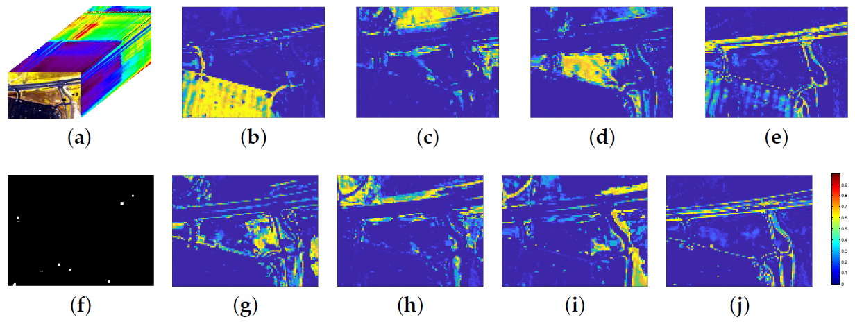
As discussed above, an accurate description of the HSI background plays a vital role in AD. The background part occupies a very high proportion of the image and in general includes multiple classes and has low-rank characteristics. AA unmixing is also a low-rank representation formulation. Therefore, each endmember obtained by the AA unmixing can be regarded as a representative of a certain background class. In fact, the AA unmixing strategy is equivalent to an effective analysis of the diversity of the background at a sub-pixel level, and the corresponding abundances can be regarded as encoded background features. After applying AA unmixing on the open source HSI data Urban (https://sites.google.com/site/feiyunzhuhomepage/datasets-ground-truths, accessed on 15 February 2015), a set of abundance maps of the different background materials of the scene were created (Figure 1). As presented in this figure, the main information conveyed by those abundance maps indicates the background. Therefore, an intuitive way to extract the anomaly target is to reconstruct the original image with the obtained endmembers and abundances summarizing the background content. Then in the reconstructed image, the difference between the reconstruction result and the background of the original image should be the smallest, and the difference between the reconstruction result and the target of the original image should be the largest. The anomaly target can be extracted with the help of this reconstruction error, and the detector can be described as follows:
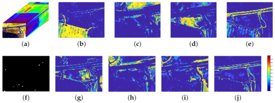
Figure 1.
Two-dimensional abundance map achieved by unmixing of a sub-image of a public hyperspectral dataset “Urban” (introduced in following Section 3.1.2). (a) Original data. (b–e) Abundance maps for the 1st, 2nd, 3rd and 4th background materials. (f) Ground truth of the abnormal targets (cars and roofs) which were embedded in the different background types. (g–j) Abundance maps for the 5th, 6th, 7th and 8th background materials.
2.2. SSRRE Based on the Sparse Representation
As discussed in Section 1, a sparse representation-based AD algorithm achieves good performance because of its ability of background feature extraction. Our proposed method will also make use of the sparse representation to improve the detection performance based on the AA unmixing strategy. For simplicity, we rewrite a 3D HSI as a 2D matrix using band sequential ordering, and denote it as (b is the band number, n is the pixel number). Each row of represents n pixels contained in a certain spectral band, and each column represents b spectral band vectors of a certain pixel. The sparse representation-based AD model is as follows:
where is the background dictionary, s is the number of atoms in the dictionary ; is the sparse representation coefficients, and each is the sparse representation coefficient with respect to the ith pixel being sparsely represented by ; represents noise. According to the sparse representing theory, when given an appropriate background dictionary, the objective function of Equation (9) can be transformed into the following optimization question:
where indicates 0 norm which constrains the sparseness of . In this model, only if is a background pixel, it can be accurately represented by . Therefore, when the sparse vector is obtained, the error between and can be used to detect the target. The detector is specifically formulated as:
where is threshold and , is considered as target, otherwise is marked as the background.
An accurate construction of the background dictionary and a well-optimized sparse representation are the two prerequisites of a precise target detection. In our previous work [33], the background dictionary is obtained by combining a local RX algorithm with a PCA learning method. To include a mixed pixel-consideration and to account for the multi-class characteristics of the background, this paper uses the endmember matrix obtained from the AA unmixing as the background dictionary. A sparse representation model based on AA spectral unmixing can be obtained as follows:
where is the endmember matrix used as the background dictionary, and is the sparse representation coefficient of the model. It has the following advantages. Firstly, the new background dictionary covers the diversity of the scene, which makes the background representation more consistent with the actual physical situation. Secondly, compared with the dictionary in [33], an AA unmixing-based dictionary has a smaller size. The dictionary size in [33] is . After unmixing, the new dictionary size is where m represents the number of endmembers, i.e., the number of background categories. Generally, the number of ground object categories in HSIs is less than the number of bands, so the size of the dictionary based on the endmember matrix is smaller.
It has been proved that introducing structural information can improve the accuracy of the coefficient estimation in sparse representation-based AD. To solve the sparse representation coefficients more accurately, a reweighted Laplace prior has been employed to model the structure in the sparse representation of HSIs as proposed in [34]. Specifically, in Equation (12) denotes the sparse representation matrix. Each column is a sparse representation vector. N indicates the sparse representation error. To model the structured sparsity during sparse representation learning, the reweighted Laplace prior is imposed on , which is a hierarchical prior. First, a matrix normal distribution is imposed on as with . I is an identity matrix with proper size, controls the noise level, the covariance matrix is a -dependent diagonal matrix, where . Then, a Gamma distribution is employed on as . By assuming N is Gaussian as with , we have the likelihood of the sparse representation model as . With the reweighted Laplace prior and the likelihood , an empirical Bayes framework is employed to learn the sparse matrix . We have the final optimization formulation for sparse learning as:
The detailed solution of Equation (13) can be found in [33,34]. Once the coefficient is obtained, the endmember based structured sparse representation reconstruction error (SSRRE) can be calculated as follows:
Instead of using only a part of the unmixing result [27], SURE simultaneously utilizes the endmember and abundance information obtained from unmixing. SSRRE utilizes endmembers as the background dictionary which describes the multi-class features of the background. The reconstruction model is capable of suppressing the target and to accurately describe the background. To effectively improve the detection performance, the proposed method uses collaborative fusion formulated as:
where is the parameter to balance the SURE part and SSRRE part, and is the segmentation threshold. When is larger than the threshold , the pixel is identified as the target; otherwise, it is a background pixel. The detailed procedure of AA spectral unmixing and structured sparse representation (AASSR) algorithm is shown in Algorithm 1.
| Algorithm 1: The Proposed AASSR Method. |
| Input: HSI , Number of endmembers m (1) Calculating the endmember matrix E and abundance matrix A using the AA spectral unmixing model: Equation (5); (2) Calculating the spectral unmixing reconstruction error (SURE) by Equation (7); (3) Obtaining the structured sparse representation model (Equation (12)) based on endmember matrix by combining the obtained endmember as background dictionary and structured sparse representation; (4) Solving the model Equation (12), and calculating the structured sparse representation reconstruction error (SSRRE) by Equation (14); (5) Calculating the reconstruction error based on SURE and SSRRE by Equation (15) Output: Reconstruction error, . |
3. Experimental Results
3.1. Datasets Description
In this paper, four datasets are utilized to evaluate the detection performance of the proposed method.
3.1.1. Simulated Dataset
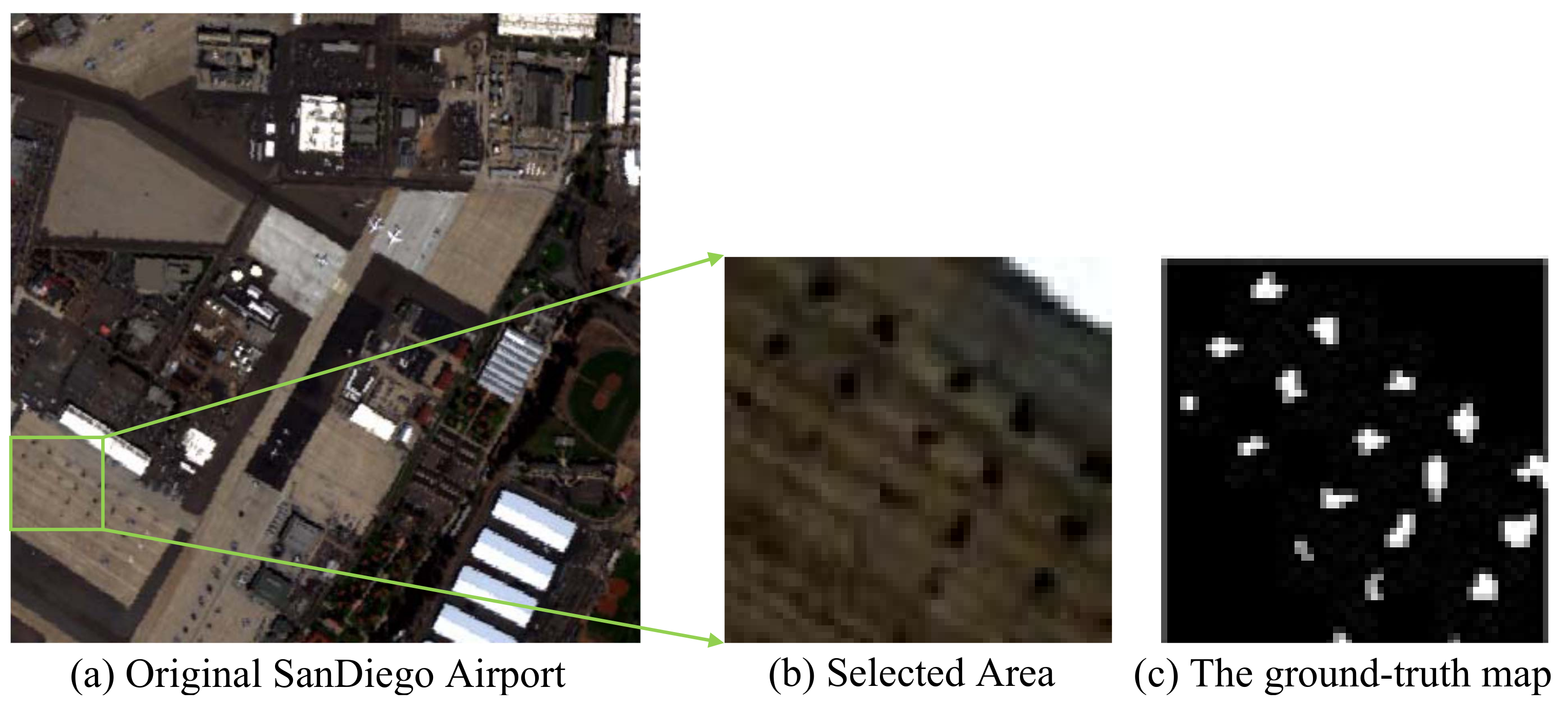
The simulated data, created using the linear weighting method, is based on real-world hyperspectral data. The real hyperspectral reflectance data was collected by AVIRIS (Airborne Visible Infrared Imaging spectrometer) at San Diego Airport, CA, USA. The spatial resolution is 3.5 m and the dataset has 224 spectral bands from 370 nm to 2510 nm. After removing the water absorption bands and bands with low signal-to-noise ratios or spurious data, 189 bands were left for further analysis. The original size of the image is pixels. In this paper, a sub-image of size pixels was selected to create simulated data. The original image and the selected area are shown in Figure 2. The method to generate the simulated data is discussed in [25,35] and will not be repeated here. The targets were embedded into the background using the target implantation technology. Specifically, according to the linear mixing model, the current background pixel q was replaced by the new pixel x which is formed as the linear combination of the target spectrum t and the current background pixel q according to the abundance fraction as follows:
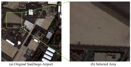
Figure 2.
San Diego Airport Dataset.
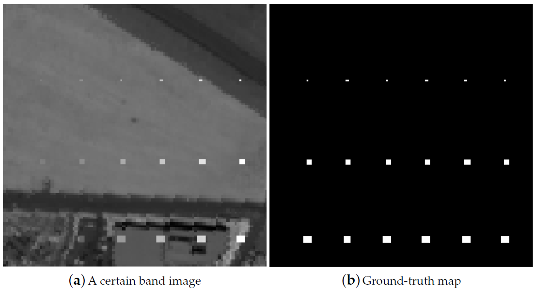
Figure 3 shows the simulated data and the ground truth. A total of 18 targets were implanted into the background and evenly distributed in the image in the form of 3 rows and 6 columns. The targets in each row are of the same size. The size (in pixel unit) of the targets, from top to bottom, is , respectively. The value of is the same in each column, from left to right, it is , respectively. The man-made aircraft in the HSI was treated as the target, and the spectrum from the aircraft pixels was extracted and used as the spectral target t.
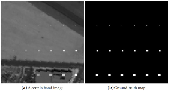
Figure 3.
Simulated dataset.
3.1.2. Real-World Dataset
There are three real-world datasets. The first is the Urban dataset shown in Figure 4a, which is collected with HYDICE. The spectral coverage is 400∼2500 nm, the spectral resolution is 10 nm, and the spatial resolution is 2 m. The entire image contains 210 bands, and has a size of pixels.This urban area has vegetation, construction, and several roads including some vehicles. The background of this dataset mainly includes trees, soil, grass, and asphalt, etc., and thus, man-made elements were used as anomaly targets. The ground reference target of the entire image is not easy to obtain [36]. A sub-image (shown in Figure 4b) of the size of from the upper right corner was selected as the test image. The low signal-to-noise ratio and water vapor absorption bands (1∼4, 76, 87, 101∼112, 136∼153, 197∼210) were removed, leaving 160 spectral bands. In this dataset, 21 man-made small targets (including cars and roofs) were used as the anomaly targets [25,37]. The anomalous targets, including cars and roofs, are embedded in different backgrounds and the anomalous target pixels include vehicles with different sizes. And the ground-truth map is shown in Figure 4c.
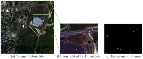
Figure 4.
Urban dataset.
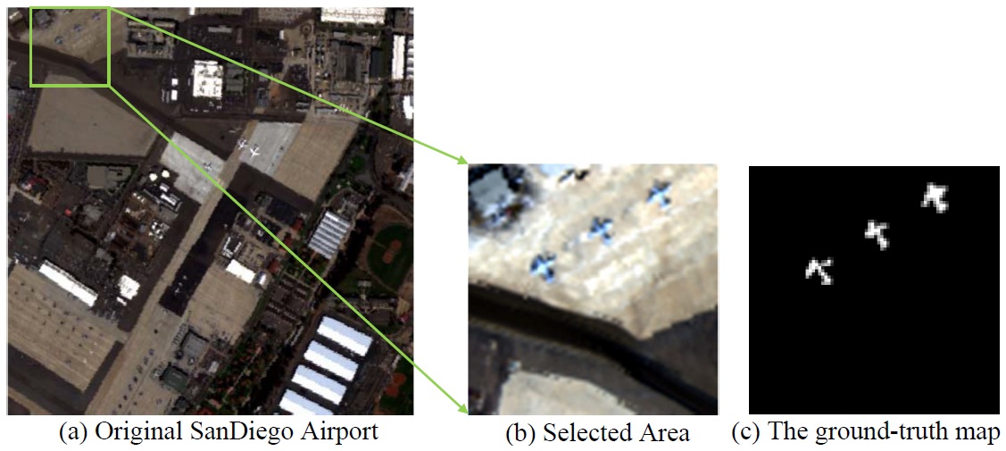
The second and third real-world datasets were selected from the San Diego Airport dataset, and the selected area and size are the same as in previous studies [13,24,25]. The second dataset is a pixels sub-image from the bottom left of the original HSI. As shown in Figure 5, the dataset is named “Sandiego60” and the aircrafts were used as the target. The third dataset is named “Sandiego80”. It is a sub-image with a size of pixels from the upper left corner of the original image. The selected scene is mainly composed of buildings with different roofs, an airport runway and a small amount of vegetation. The aircrafts represent the anomaly targets. The selected area and the groundtruth map are shown in Figure 6.

Figure 5.
Sandiego60 dataset.

Figure 6.
Sandiego80 dataset.
3.2. Comparison Methods
To evaluate the performance of the proposed method, eight state-of-the-art methods were employed for comparison. They are GlobalRX (GRX) [4], LocalRX (LRX) [6], Background Joint Sparse Representation Detection (BJSRD) [20], Local Summation Anomaly Detector (LSAD) [38], Collaborative Representation for Hyperspectral Anomaly Detection (CRD) [39], Cluster-Based Anomaly Detector (CBAD) [7], Low-Rank and Sparse Representation (LRASR) [25], Abundance and Dictionary-based Low Rank Decomposition (ADLR) [27]. Among those methods, a Matlab Toolkit (https://github.com/davidkun/HyperSpectralToolbox, accessed on 15 February 2016) was used to run the first two state-in-art methods. The code of CRD algorithm is available at https://sites.google.com/site/godecomposition/code, accessed on 15 June 2017. The codes of other methods are not accessible. However, the low-rank representation and clustering used by the other methods were realized by utilizing the corresponding toolboxes in Matlab.
(a). GRX and LRX are the benchmark algorithms to be compared. They assume that the background obeys a fixed model in AD.
(b). BJSRD is a new AD algorithm based on the sparse representation theory. This algorithm uses the traditional OMP algorithm [40] for sparse coefficients optimization.
(c). The LSAD algorithm is similar to the single-window LRX algorithm. It uses a multi-window sliding filter to obtain various spatial distributions of pixels adjacent to the cells to be measured, and this local aggregating strategy integrates spectral and spatial information to improve the detection performance.
(d). The CRD algorithm is based on the principle that each pixel in the background can be approximated by its spatial neighborhood, while the anomaly target cannot. The background estimation is realized by sliding the double window to approximate each central pixel as a linear combination of the surrounding samples. The anomaly target is extracted based on the residual image obtained by subtracting the predicted background from the original HSI.
(e). The CBAD method divides the HSI into clusters using the Gaussian mixture model (GMM). The Mahalanobis distance is then calculated between the pixel under test and the center of each class. The anomaly targets are those with a distance larger than a pre-defined threshold.
(f). LRASR decomposes the background into low-rank and sparse matrices, and the anomaly target is included in the residual. The k-means clustering method is used for dictionary construction.
(g). ADLRS is a typical anomaly target detection method based on spectral unmixing. This method first uses the traditional MV-NMF to unmix the input HSI. It then constructs the dictionary with clusters obtained from the abundance matrix using a meanshift clustering algorithm. The dictionary is further used in a low-rank matrix decomposition model to divide the abundance matrix into the low-rank part (background) and the sparse part (the target). The anomaly target is extracted from the sparse part. Similar to the proposed method, ADLRS analyzes the HSI at a sub-pixel level using spectral unmixing.
Since the proposed method integrates SURE and SSRRE for AD, the detection results are presented separately in the experiments, and they are defined as the SURE detector (SUREAD) and the SSRRE detector (SSRREAD).
3.3. Experimental Results and Analysis
The Receiver Operating Characteristic (ROC) curve generated on a per pixel basis and the Area Under the ROC Curve (AUC) indexes are used to evaluate the methods. Given a threshold, the detection result can be transformed to a binary image, where value 1 represents that targets are present in the pixel and value 0 represents that targets are absent. Based on the ground truth, the ROC curve presents the varying trend between the detection probability and false alarm rate by taking all possible thresholds. and are defined as
where represents the number of anomalous target pixels detected with certain threshold, represents the total number of anomalous target pixels in the image, represents the number of background pixels having been detected and represents the total pixel number of the image. The parameters with respect to a more superior detector would lie nearer the top left of the ROC curve or are with a larger area under the curve (AUC). The AUC is also quantitatively computed to evaluate the detection performance for further validation. A detailed explanation about these two indexes can be found in [41].
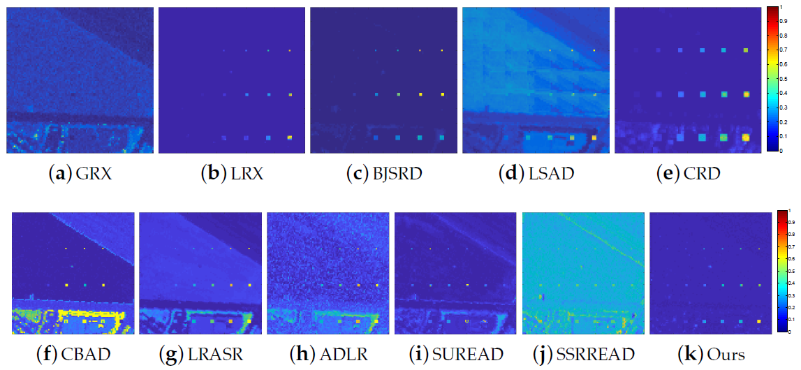
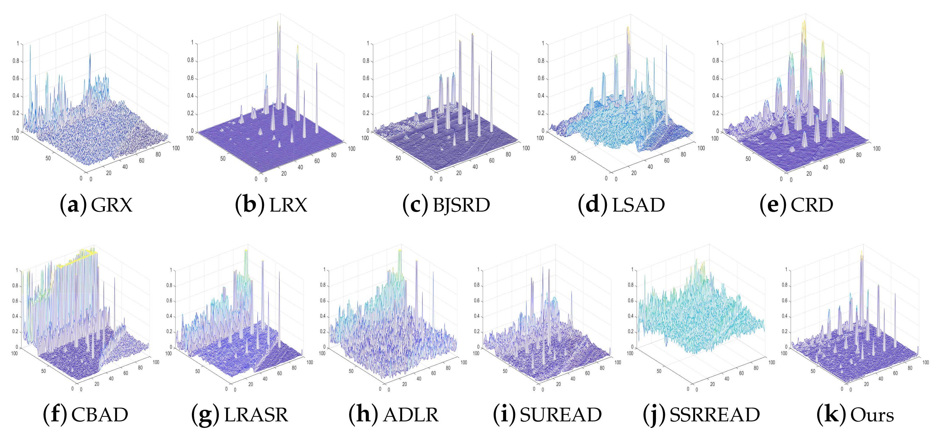
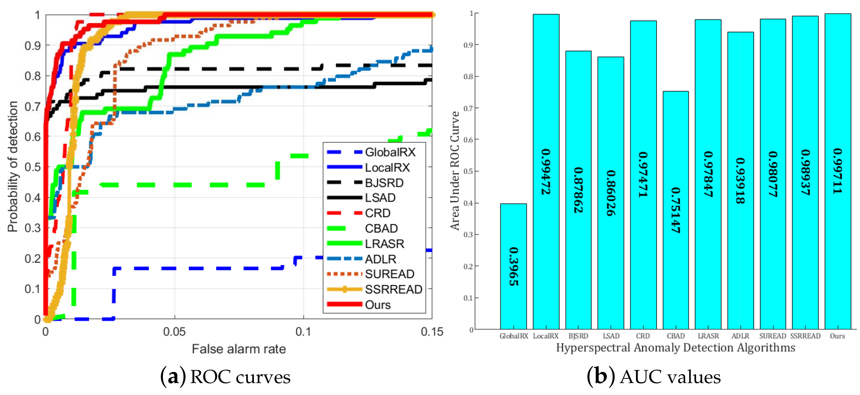
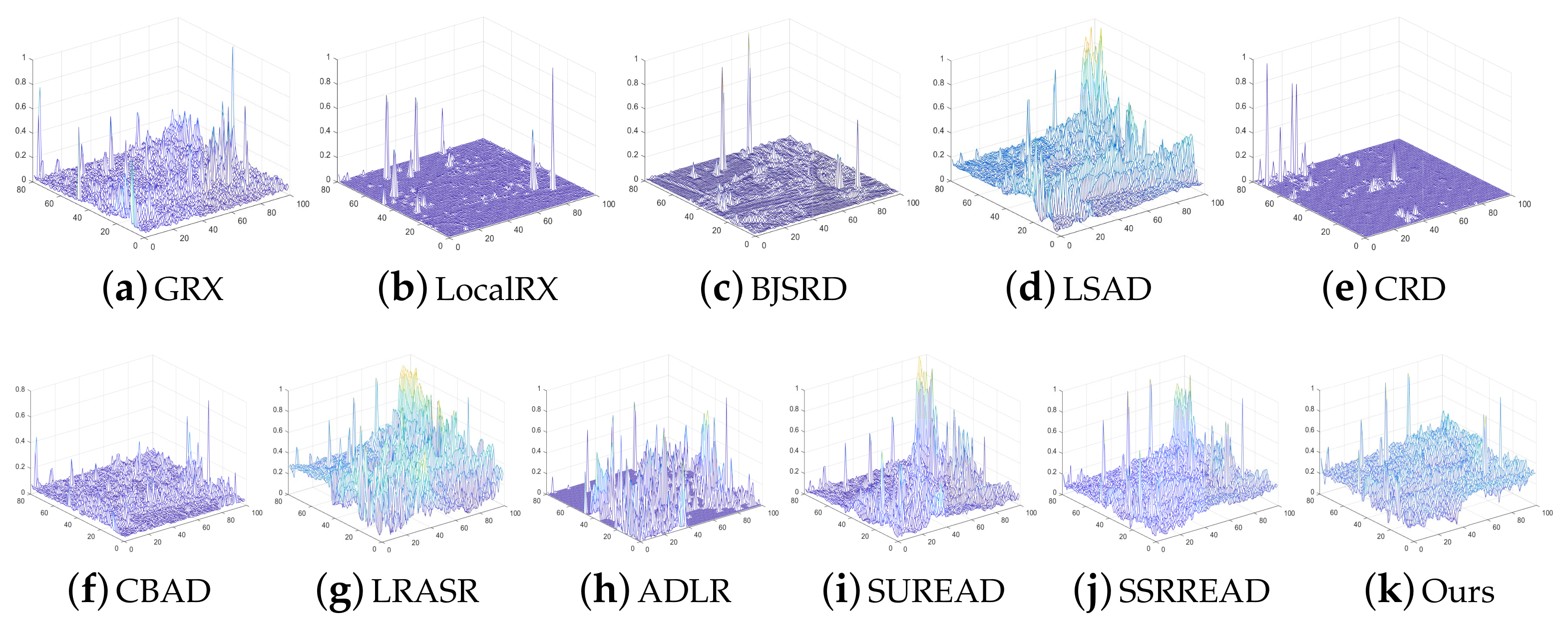
Figure 7 and Figure 8 present the detection probabilities of the methods on the simulated data in the 2-D and 3-D space. The targets in this dataset were obtained as a linear combination of the background pixels and the target spectrum. Thus, the mixed pixels in the image account for a high proportion. Those two figures show that the simulated targets detected by our proposed method (see Figure 7k) were visually closest to the ground truth shown in Figure 3b. It is further confirmed by the visible number of detected targets in Figure 8k. The results of SURE, shown in Figure 7i, were achieved by reconstructing the original image via AA unmixing. The results show that the method managed to suppress the background to a large extent. After the dictionary was constructed by the endmembers and inserted into the structured sparse representation model for AD, the detection probability of SSRRE is shown in Figure 7j. Even if the targets are highlighted against the background, there are also false alarms. Figure 7k shows the final fused results of SURE and SSRRE, which realize the background suppression and target highlighting at the same time. The ROC curves and AUC values of the detection results on the simulated data are shown in Figure 9. The proposed algorithm achieved an highest AUC value of 0.99711 indicating its effectiveness, even though the LRX was very approaching.
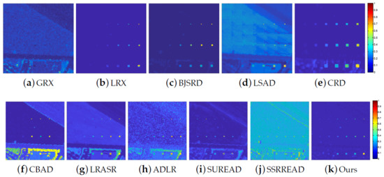
Figure 7.
2-D target probability color maps of the detection algorithms for the simulated dataset.

Figure 8.
3-D mesh of the detection algorithms for the simulated dataset.

Figure 9.
ROC curves and AUC values for the simulated dataset.
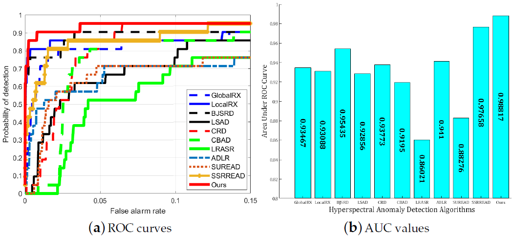
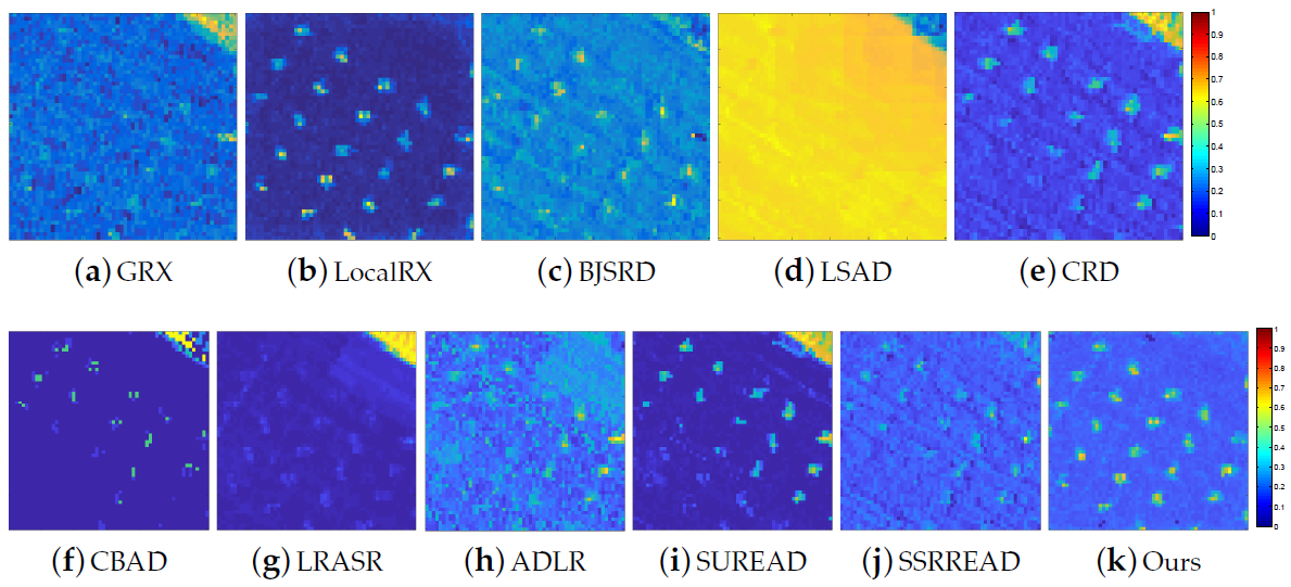
For the Urban data, the detection results expressed in a 2D and 3-D space are shown in Figure 10 and Figure 11, and the corresponding ROC and AUC results are summarized in Figure 12. It is clear the detection results via SURE (shown in the Figure 10i) have not achieved background suppression. However, when combined with SSRRE, the targets can be prominently highlighted as shown in the Figure 10k. The AUC value of the proposed method is the highest at 0.98817 (Figure 12) which dominantly surpassed the other methods. Different from the results achieved on the simulated dataset, it was in particular far more than the LRX method on the Urban data.
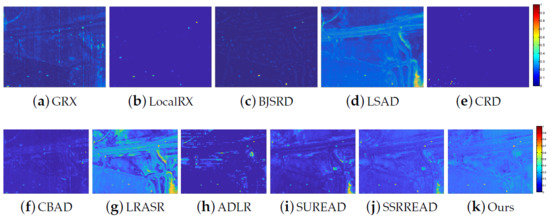
Figure 10.
2-D target probability color maps of the detection algorithms for the Urban dataset.

Figure 11.
3-D mesh of the detection algorithms for the Urban dataset.

Figure 12.
ROC curves and AUC values for the Urban dataset.
The last two real-world datasets, Sandiego60 and Sandiego80, are both from the San Diego Airport dataset. The 18 aircrafts in Sandiego60 are smaller in size and the study area has a relatively low background complexity. There are three aircrafts in Sandiego80, larger than those in Sandiego60, but the background objects presented are more challenging.
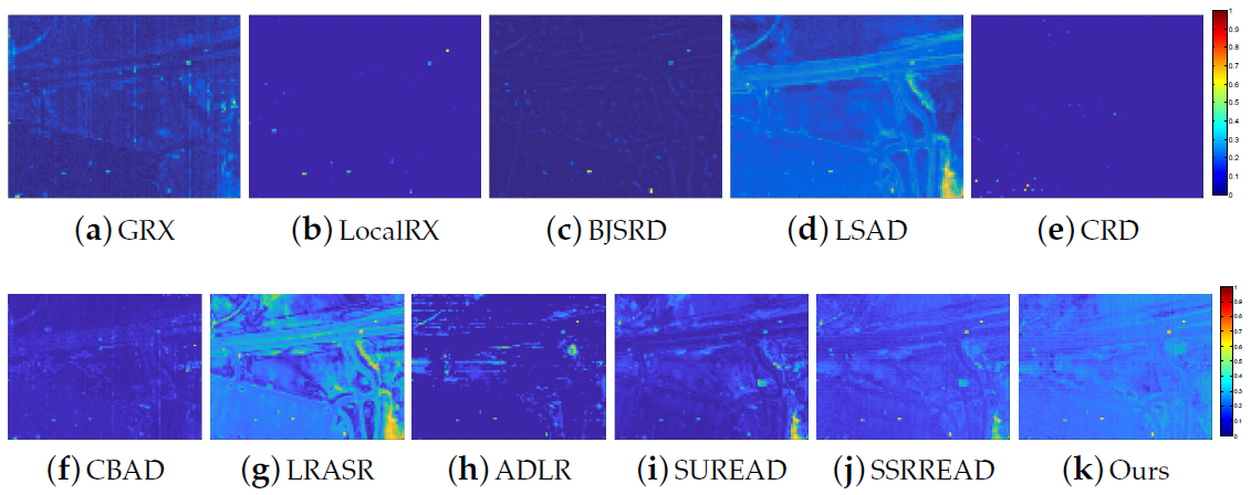
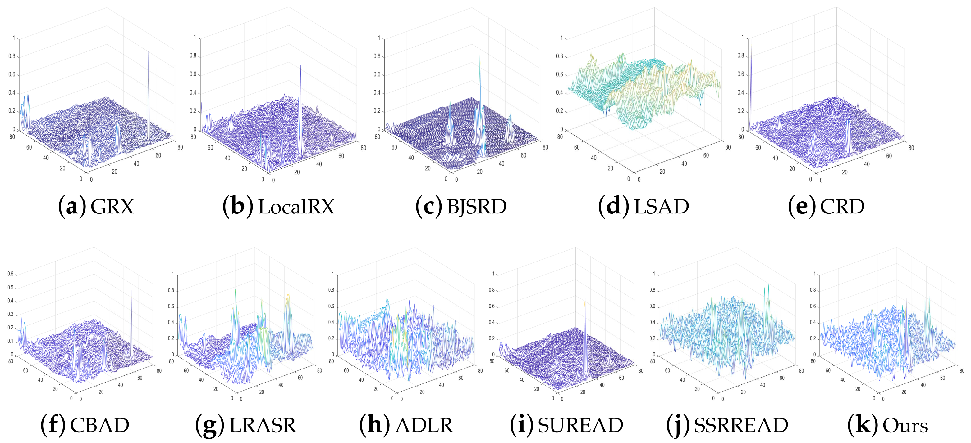
The detection results, ROC cures and AUC values achieved on Sandiego60 are shown in the Figure 13, Figure 14 and Figure 15. The detection results, ROC cures and AUC values achieved on Sandiego80 are shown in the Figure 16, Figure 17 and Figure 18. The traditional statistics-based methods (such as GRX, LRX, LSAD) assume that the background obeys a fixed model and as a result, their detection accuracies are low. Although representation-based methods (such as CRD, LRASR) can better describe the background features, they do not consider spectral mixing and their detection results are not satisfactory. Spectral unmixing based ADLR method only uses the abundance matrix after unmixing, which leads to poor detection results. The proposed algorithm employs the sparse representation theory to model the background features accurately, and also collaboratively considers the mixed pixel characteristic at a sub-pixel level. The best AUC values present more precise comparisons, all the detection methods include ours worked better on Sandiego80 data than that on Sandiego60 data. Under this condition, the best AUC value of our method obtained on Sandiego80 data surpassed that of the second-ranked method with more value.

Figure 13.
2-D target probability color maps of the detection algorithms for the Sandiego60 dataset.
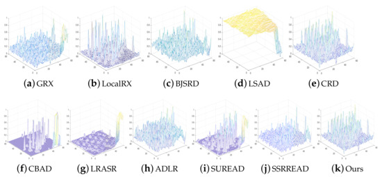
Figure 14.
3-D mesh of the detection algorithms for the Sandiego60 dataset.
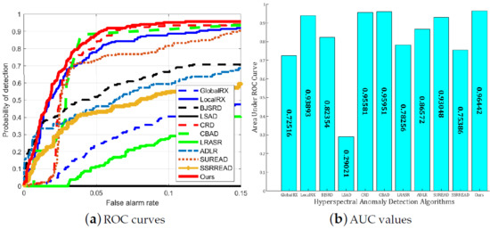
Figure 15.
ROC curves and AUC values for the Sandiego60 dataset.
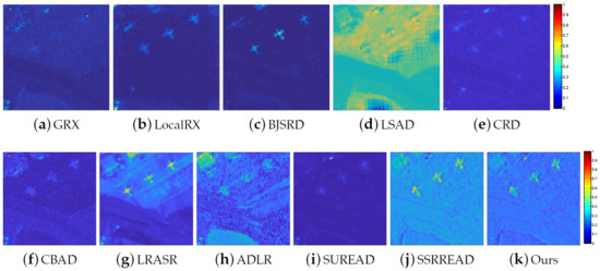
Figure 16.
2-D target probability color maps of the detection algorithms for the Sandiego80 dataset.
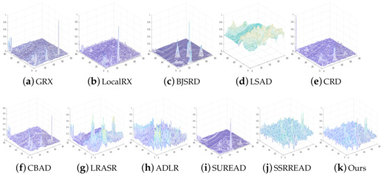
Figure 17.
3-D mesh of the detection algorithms for the Sandiego80 dataset.
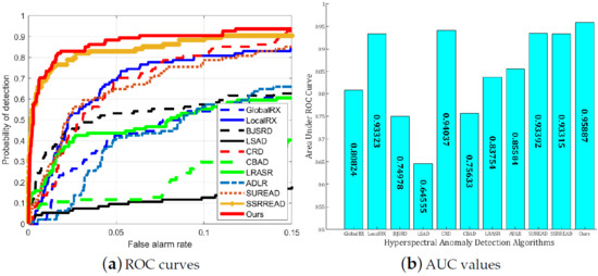
Figure 18.
ROC curves and AUC values for the Sandiego80 dataset.
To evaluate the computational complexity of the proposed method, the running times of all methods are summarized in Table 1. All experiments were implemented with MATLAB software on the laptop which has 16 GB RAM and the CPU as 64-bit Intel Core i7-9750H working at 2.6-GHz. It is obvious that as the data size increases, the running time of all algorithms increases. Compared with other methods, the time consumed by the proposed method is moderate and acceptable.

Table 1.
Running Times (s) of All Methods for All Datasets.
3.4. Analysis of Parameters and Unmixing Method
In this section, the main parameters involved in the proposed algorithm are briefly summarized and analyzed. In addition, the AA unmixing method was compared with the well-known Minimum Volume constrained Nonnegative Matrix Factorization (MV-NMF) spectral unmixing method [27] on all of the datasets to indirectly verify the effectiveness of the proposed method.
3.4.1. Parameter Analysis
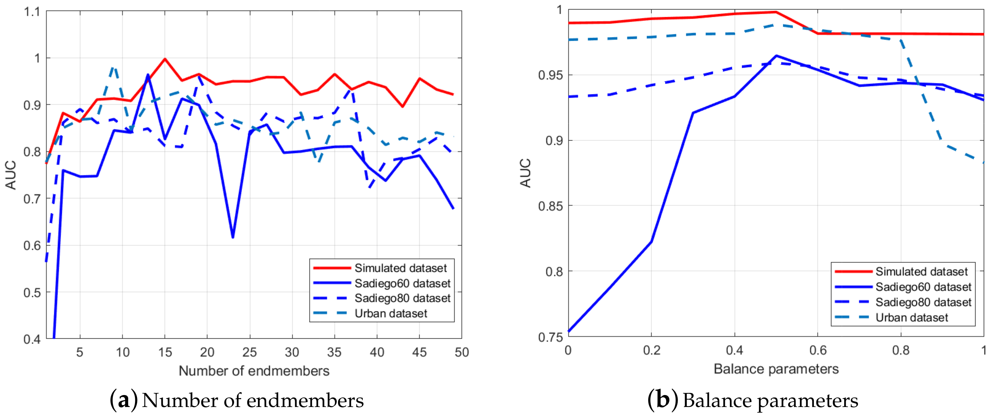
The main parameters of the proposed method are the number of endmembers m and the balance parameter in the final fusion error. When analyzing the influence of the varied number of endmembers on the detection performance in terms of AUC, a total of 25 values were taken in the range of 1–50 at an interval of 2 to calculate the AUC value with the balance parameter fixed at the best value of . Figure 19a presents the AUC values obtained by the proposed method with varied numbers of the endmember. It can be seen that when the number of endmembers is too small or too large, their representation of the background information results in poor detection performance on all datasets. Different levels of fluctuation are observed on different datasets. Comparatively, relatively smaller variation was observed on the synthetic data than that on the other three real data. From Figure 19a, it can be seen that the proposed detection method performs well on the simulated data when the endmember number is in the range of 10–18. For the Urban datasets, the performance is better when the number of endmembers is 8–10. On the two subsets of San Diego data, more number of endmembers was needed for our method to represent the background well and get a promising detection result of Sandiego80 subset compared to that of Sandiego60 subset.
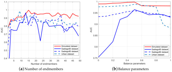
Figure 19.
Analysis of main parameters.
As for the balance parameter, 11 values were selected in the range of at a step of . As shown in Figure 19b, good results are obtained at values near 0.5. So the presented best results achieved by our method on all the datasets were all obtained with the balance parameter set as 0.5. When the balance parameter takes values between 0 and 1, they represent special cases where only a single reconstruction error is used to extract anomaly targets. In such cases, SUREAD or SSRREAD are working independently. Note that the detection performance is poor in these two special cases. Figure 19b further demonstrates the necessity to fuse these two parts.
3.4.2. Unmixing Method Analysis
The proposed method is inspired by the AD detection strategy based on spectral unmixing, which attempts to analyze and extract the background features at a sub-pixel level. The proposed method adopts the AA spectral unmixing strategy. To analyze the advantages of an AA unmixing algorithm, we replaced the AA unmixing with the well-known MVNMF [27]. In order to comprehensively evaluate the performance, a total of 25 values were taken between 1–50 at intervals of 2 to calculate the AUC value. Figure 20 shows the detection performance in terms of AUC obtained by AA and MVNMF on each dataset. It is apparent that the AA unmixing based AD outperforms the MV-NMF based AD under every background representation condition. This shows the AA unmixing method is the right choice for AD.

Figure 20.
Detection accuracy of different unmixing methods.
4. Discussion
Anormaly detection through hyperspectral remote sensing technique is a significant application task demanded for both military and civilian monitoring. To accurately identify the abnormal targets, a good representation of the background information plays a vital role. This task is particular difficult due to the fact that mixed pixels commonly exist in the remote sensing images. Available studies have consider this problem by using spectral unmixing approach to generate more representative features used for AD. Simple low-rank representation methods, such as PCA [20] and MN-NMF [27], have been adopted for the background information learning, which render the improvement of detection performance being limited. In this study, a well-constrained spectral unmiixng model of AA is introduced to conduct spectral unmixing which is mainly intended for representative signature extractions for direct representation of background information. Here, we discuss the implications of our results with respect to the applicability of AA unmixing model for the background representation, the key parameter in spectral unmixing and the complexity of background.
In concern of the mixed pixels in hyperspectral images, the precise target detection needs to be conducted at a sub-pixel level. Therefore spectral unmixing is a essential step used for accurate target detection. As has been mentioned in previous section that AD methods based on low rank and sparse representation have been proposed to decompose the HSI into the low-rank and sparse parts. It assumes that the target can be extracted from the sparse part if the background has low-rank characteristics and the target is sparse [21,22]. The fact that AA also enables low-rank and sparse representations motivates us to conduct this initial exploration of using AA unmixing to generate representative background dictionary. From a physical point of view, the model of AA finds distinct patterns in the data [28]. It has been demonstrated to be of potential value in spectral unmixing which is used to generate pure representative endmembers of the data. It is well-known for those who work on spectral unmixing that mixed data is distributed as simplex in the low dimensional feature space and the pure endmembers are located as the vertices of the simplex in idea conditions (in practical cases, it would not be a very regular simplex structure).The archetypes obtained by the AA associated models are the main representatives for the different class types of the data. Abnormal targets are, in general, very small and occupy only a small proportion of the image which also would be very different from the background materials. Thus, the targets may distribute far from the background data samples which means AA can be used to get endmember signatures for background representation with proper setting of number of endmembers. Figure 1 is a case which proves this. As has also been mentioned, the well constrained AA is superior to MV-NMF [27] in endmember extraction. The practical evaluation is in accordance with such theoretical assumptions referring to what is presented in Figure 20. Moreover, all the detection results achieved on both simulated and real datasets verify the effective of our AA unmixing based AD methods.
The number of endmembers in fact plays a vital role in our study with our initial trying to use AA unmixing technique to provide a low dimension representation of the background data. As is observed in Figure 19a, the method is a little sensitive to this parameter setting. Many variants of NMF models have been developed for the unsupervised unmixing where the endmember number is also often provided as prior information. So we also manually set this number with a general understanding of the background from available studies. Therefore, it needs to mention that a priori knowledge of the background is needed to ensure a good behavior of the proposed method and consequently interpretable and exploitable results at output.
A priori knowledge of the background relates to know about the background complexity. It is difficult to give a clear definition of the “complex background”. However, it at least refers to the background where there are more different classes than the targets. What’s more important, heterogeneous region existed obviously. Among the four experimental datasets, the Urban data and Sandiego80 are assumed as more complex. This is because the targets in the simulated data and in Sandiego80 data are less (more sparse) than that in the other two datasets, and the backgrounds in the former two datasets have more heterogeneous regions than the latter ones. As comparison, dominant and large homogeneous regions can be found in the simulated and Sandiego60 datasets. So the former two datasets were assumed to be more complex. We have pointed out that our method is mainly intended for complex background cases. The best AUC of each method achieved on those four datasets also indicated that the traditional statistical modeling based AD methods (such as GRX, LRX) fell more behind our method on the former datasets, whereas in the case of the latter two datasets its accuracy approached the accuracy of our methods. However, Figure 19a also shows the latter two datasets needed more endmembers used in the proposed algorithm though they were assumed to have simple backgrounds. In fact, this is more possible as for the intra-class spectral variability. As large homogeneous regions can be observed in those two scenes, the intra-class spectral variability is a more dominant problem in such a scene than that in a scene with more heterogeneous regions. So there must be multiple endmembers from the same background types, which under certain condition, would also decrease the chance to include target in the endmembers extraction of our method. It is recommended that question, the related factors and verification be studied more deeply in the future. In addition, this also throw light on the future study to extend our study by exploration of effective strategy to realize multiple endmembers extraction for better background representation for AD.
5. Conclusions
Mixed pixels in HSIs hinder the accurate detection of background features in AD analysis. In this paper, a novel AASSR target detection method is proposed to extract the anomaly target at a sub-pixel level. Specifically, a well constrained AA unmixing method is deployed to obtain representative background endmembers. By using the AA unmixing model, the unmixing reconstruction error can be used for AD. Moreover, The endmembers obtained by AA unmixing was also used as a background dictionary in the structured sparse representation model for AD. The final target detector is realized using both unmixing error and the sparse representation error which are fused into a linear weighted framework to provide the final AD results. Experiments on four hyperspectral datasets and comparisons with ten methods show the potential of the proposed method. Basing the parameter analysis results, the use of AA for AD is demonstrated of great priority over the state-in-art MV-NMF unmixing strategy for AD. However, at the same time, it also needs to be highlighted that our initial trying with AA for AD needs a priori knowledge of the background information to get a promising result. The experimental results indicate that on the complex background which has more class types and heterogeneous region, our method is observed as having more potential. For the background with large homogeneous regions, a large value should be set for the endmember number. The spectral variability (intra-class or inter-class) would be a potential influencing factor which demands further investigation.
Author Contributions
Methodology, F.L. and G.Z.; software, F.L.; validation, F.L. and G.Z.; data curation, F.L.; writing—original draft preparation, F.L. and G.Z.; writing—review and editing, X.Z., K.L. and J.C.-W.C.; funding acquisition, G.Z. All authors have read and agreed to the published version of the manuscript.
Funding
This research was funded by the National Natural Science Foundation of China under Grant (61701123), Guangdong Provincial Key Laboratory of Cyber-Physical System under Grant (2020B1212060069), High Resolution Earth Observation Major Project under Grant (83-Y40G33-9001-18/20).
Institutional Review Board Statement
Not applicable.
Informed Consent Statement
Not applicable.
Acknowledgments
This work was sponsored in part by the National Natural Science Foundation of China under Grant (61701123), Guangdong Provincial Key Laboratory of Cyber-Physical System under Grant (2020B1212060069), High Resolution Earth Observation Major Project under Grant (83-Y40G33-9001-18/20).
Conflicts of Interest
The authors declare no conflict of interest.
References
- Ma, J.; Sun, D.W.; Pu, H.; Cheng, J.H.; Wei, Q. Advanced Techniques for Hyperspectral Imaging in the Food Industry: Principles and Recent Applications. Annu. Rev. Food Sci. Technol. 2019, 39, 197–220. [Google Scholar] [CrossRef]
- Basantia, N.; Nollet, L.M.; Kamruzzaman, M. Hyperspectral Imaging Analysis and Applications for Food Quality; CRC Press: Boca Raton, FL, USA, 2018. [Google Scholar]
- Shaw, G.; Manolakis, D. Signal Processing for Hyperspectral Image Exploitation. Signal Process. Mag. IEEE 2019, 19, 12–16. [Google Scholar] [CrossRef]
- Reed, I.S.; Yu, X. Adaptive Multiple-band CFAR Detection of an Optical Pattern with Unknown Spectral Distribution. IEEE Trans. Acoust. Speech Signal Process. 1990, 38, 1760–1770. [Google Scholar] [CrossRef]
- Qu, Y.; Guo, R.; Wang, W.; Qi, H.; Ayhan, B.; Kwan, C.; Vance, S. Anomaly Detection in Hyperspectral Images Through Spectral Unmixing and Low Rank Decomposition. In Proceedings of the 2016 IEEE International Geoscience and Remote Sensing Symposium (IGARSS), Beijing, China, 10–15 July 2016; pp. 1855–1858. [Google Scholar]
- Borghys, D.; Kåsen, I.; Achard, V.; Perneel, C. Comparative Evaluation of Hyperspectral Anomaly Detectors in Different Types of Background. In Proceedings of the SPIE Defense, Security, and Sensing, Baltimore, MD, USA, 23–27 April 2012; Volume 83902. [Google Scholar]
- Carlotto, M.J. A Cluster-Based Approach for Detecting Man-Made Objects and Changes in Imagery. IEEE Trans. Geosci. Remote Sens. 2005, 43, 374–387. [Google Scholar] [CrossRef]
- Zhang, X.; Wen, G.; Dai, W. A Tensor Decomposition-Based Anomaly Detection Algorithm for Hyperspectral Image. IEEE Trans. Geosci. Remote Sens. 2016, 54, 5801–5820. [Google Scholar] [CrossRef]
- Veracini, T.; Matteoli, S.; Diani, M.; Corsini, G. Fully Unsupervised Learning of Gaussian Mixtures for Anomaly Detection in Hyperspectral Imagery. In Proceedings of the 2009 Ninth International Conference on Intelligent Systems Design and Applications, Pisa, Italy, 30 November–2 December 2009; pp. 596–601. [Google Scholar]
- Guo, Q.; Zhang, B.; Ran, Q.; Gao, L.; Li, J.; Plaza, A. Weighted-Rxd and Linear Filter-Based RXD: Improving Background Statistics Estimation for Anomaly Detection in Hyperspectral Imagery. IEEE J. Sel. Top. Appl. Earth Obs. Remote Sens. 2014, 7, 2351–2366. [Google Scholar] [CrossRef]
- Kwon, H.; Nasrabadi, N.M. Kernel RX-Algorithm: A Nonlinear Anomaly Detector for Hyperspectral Imagery. IEEE Trans. Geosci. Remote Sens. 2005, 43, 388–397. [Google Scholar] [CrossRef]
- Banerjee, A.; Burlina, P.; Diehl, C. A Support Vector Method for Anomaly Detection in Hyperspectral Imagery. IEEE Trans. Geosci. Remote Sens. 2006, 44, 2282. [Google Scholar] [CrossRef]
- Zhao, R.; Du, B.; Zhang, L. A Robust Nonlinear Hyperspectral Anomaly Detection Approach. IEEE J. Sel. Top. Appl. Earth Obs. Remote Sens. 2014, 7, 1227–1234. [Google Scholar] [CrossRef]
- Gao, Y.; Cheng, T.; Wang, B. Nonlinear Anomaly Detection Based on Spectral-Spatial Composite Kernel for Hyperspectral Images. IEEE Geosci. Remote Sens. Lett. 2021, 18, 1269–1273. [Google Scholar] [CrossRef]
- Song, S.; Zhou, H.; Qin, H.; Qian, K.; Cheng, K.; Qian, J. Hyperspectral Image Anomaly Detecting Based on Kernel Independent Component Analysis. In Proceedings of the Fourth Seminar on Novel Optoelectronic Detection Technology and Application, Nanjing, China, 24–26 October 2018; Volume 10697. [Google Scholar]
- Zhou, J.; Kwan, C.; Ayhan, B.; Eismann, M.T. A Novel Cluster Kernel RX Algorithm for Anomaly and Change Detection Using Hyperspectral Images. IEEE Trans. Geosci. Remote Sens. 2016, 54, 6497–6504. [Google Scholar] [CrossRef]
- Chang, C.I. Orthogonal Subspace Projection (OSP) Revisited: A Comprehensive Study and Analysis. IEEE Trans. Geosci. Remote Sens. 2005, 43, 502–518. [Google Scholar] [CrossRef]
- Chen, Y.; Nasrabadi, N.M.; Tran, T.D. Sparse Representation for Target Detection in Hyperspectral Imagery. IEEE J. Sel. Top. Signal Process. 2011, 5, 629–640. [Google Scholar] [CrossRef]
- Wright, J.; Ma, Y.; Mairal, J.; Sapiro, G.; Huang, T.S.; Yan, S. Sparse Representation for Computer Vision and Pattern Recognition. Proc. IEEE 2010, 98, 1031–1044. [Google Scholar] [CrossRef] [Green Version]
- Li, J.; Zhang, H.; Zhang, L.; Ma, L. Hyperspectral Anomaly Detection by the Use of Background Joint Sparse Representation. IEEE J. Sel. Top. Appl. Earth Obs. Remote Sens. 2015, 8, 2523–2533. [Google Scholar] [CrossRef]
- Cheng, T.; Wang, B. Manifold Regularized Low-Rank Representation for Hyperspectral Anomaly Detection. In Proceedings of the IEEE International Geoscience and Remote Sensing Symposium, Valencia, Spain, 22–27 July 2018; pp. 2853–2856. [Google Scholar]
- Niu, Y.; Wang, B. Hyperspectral Anomaly Detection Based on Low-Rank Representation and Learned Dictionary. Remote Sens. 2016, 8, 289. [Google Scholar] [CrossRef] [Green Version]
- Sun, W.; Liu, C.; Li, J.; Lai, Y.M.; Li, W. Low-Rank and Sparse Matrix Decomposition-Based Anomaly Detection for Hyperspectral Imagery. J. Appl. Remote Sens. 2014, 8, 083641. [Google Scholar] [CrossRef]
- Zhang, Y.; Du, B.; Zhang, L.; Wang, S. A Low-Rank and Sparse Matrix Decomposition-Based Mahalanobis Distance Method for Hyperspectral Anomaly Detection. IEEE Trans. Geosci. Remote Sens. 2016, 54, 1376–1389. [Google Scholar] [CrossRef]
- Xu, Y.; Wu, Z.; Li, J.; Plaza, A.; Wei, Z. Anomaly Detection in Hyperspectral Images Based on Low-Rank and Sparse Representation. IEEE Trans. Geosci. Remote Sens. 2016, 54, 1990–2000. [Google Scholar] [CrossRef]
- Erdinç, A.; Aksoy, S. Anomaly Detection With Sparse Unmixing and Gaussian Mixture Modeling of Hyperspectral Images. In Proceedings of the 2015 IEEE International Geoscience and Remote Sensing Symposium (IGARSS), Milan, Italy, 26–31 July 2015; pp. 5035–5038. [Google Scholar]
- Qu, Y.; Wang, W.; Guo, R.; Ayhan, B.; Kwan, C.; Vance, S.; Qi, H. Hyperspectral Anomaly Detection Through Spectral Unmixing and Dictionary-Based Low-Rank Decomposition. IEEE Trans. Geosci. Remote Sens. 2018, 56, 4391–4405. [Google Scholar] [CrossRef]
- Mrup, M.; Hansen, L.K. Archetypal Analysis for Machine Learning and Data Mining. Neurocomputing 2012, 80, 54–63. [Google Scholar] [CrossRef]
- Zhao, G.; Cheng, L.; Wu, H.; Hui, L.; Li, X. Relative Attribute Based Unmixing. In Proceedings of the IGARSS 2018—2018 IEEE International Geoscience and Remote Sensing Symposium, Valencia, Spain, 22–27 July 2018. [Google Scholar]
- Zhao, C.; Zhao, G.; Jia, X. Hyperspectral Image Unmixing Based on Fast Kernel Archetypal Analysis. IEEE J. Sel. Top. Appl. Earth Obs. Remote Sens. 2017, 10, 331–346. [Google Scholar] [CrossRef]
- Cutler, A.; Breiman, L. Archetypal Analysis. Technometrics 1994, 36, 338–347. [Google Scholar] [CrossRef]
- Lin, C.J. Projected Gradient Methods for Nonnegative Matrix Factorization. Neural Comput. 2007, 19, 2756–2779. [Google Scholar] [CrossRef] [Green Version]
- Li, F.; Zhang, X.; Zhang, L.; Jiang, D.; Zhang, Y. Exploiting Structured Sparsity for Hyperspectral Anomaly Detection. IEEE Trans. Geosci. Remote Sens. 2018, 56, 4050–4064. [Google Scholar] [CrossRef]
- Zhang, L.; Wei, W.; Zhang, Y.; Tian, C.; Li, F. Reweighted Laplace Prior Based Hyperspectral Compressive Sensing for Unknown Sparsity. In Proceedings of the IEEE Conference on Computer Vision and Pattern Recognition, Boston, MA, USA, 18–22 June 2018; pp. 4050–4064. [Google Scholar]
- Stefanou, M.S.; Kerekes, J.P. A Method for Assessing Spectral Image Utility. IEEE Trans. Geosci. Remote Sens. 2009, 47, 1698–1706. [Google Scholar] [CrossRef]
- Ma, L.; Crawford, M.M.; Tian, J. Anomaly Detection for Hyperspectral Images Based on Robust Locally Linear Embedding. J. Infrared Millim. Terahertz Waves. 2010, 31, 753–762. [Google Scholar] [CrossRef]
- Du, B.; Zhang, L. A Discriminative Metric Learning Based Anomaly Detection Method. IEEE Trans. Geosci. Remote Sens. 2010, 52, 6844–6857. [Google Scholar]
- Du, B.; Zhao, R.; Zhang, L.; Zhang, L. A Spectral-Spatial Based Local Summation Anomaly Detection Method for Hyperspectral Images. Signal Process. 2016, 124, 115–131. [Google Scholar] [CrossRef]
- Li, W.; Du, Q. Collaborative Representation for Hyperspectral Anomaly Detection. IEEE Trans. Geosci. Remote Sens. 2015, 53, 1463–1474. [Google Scholar] [CrossRef]
- Elad, M. Sparse and Redundant Representations—From Theory to Applications in Signal and Image Processing; Springer Publishing Company, Incorporated: New York, NY, USA, 2015. [Google Scholar]
- Fawcett, T. An Introduction to ROC Analysis. Pattern Recognit. Lett. 2005, 27, 861–874. [Google Scholar] [CrossRef]
Publisher’s Note: MDPI stays neutral with regard to jurisdictional claims in published maps and institutional affiliations. |
© 2021 by the authors. Licensee MDPI, Basel, Switzerland. This article is an open access article distributed under the terms and conditions of the Creative Commons Attribution (CC BY) license (https://creativecommons.org/licenses/by/4.0/).

