
BiFA-YOLO: A Novel YOLO-Based Method for Arbitrary-Oriented Ship Detection in High-Resolution SAR Images


College of Electronic Science and Technology, National University of Defense Technology, Changsha 410073, China
*
Author to whom correspondence should be addressed.
Remote Sens. 2021, 13(21), 4209; https://doi.org/10.3390/rs13214209
Submission received: 25 September 2021
/
Revised: 16 October 2021
/
Accepted: 19 October 2021
/
Published: 20 October 2021
(This article belongs to the Special Issue Object-Level Remote Sensing Image Information Extraction and Applications)
Abstract
:Due to its great application value in the military and civilian fields, ship detection in synthetic aperture radar (SAR) images has always attracted much attention. However, ship targets in High-Resolution (HR) SAR images show the significant characteristics of multi-scale, arbitrary directions and dense arrangement, posing enormous challenges to detect ships quickly and accurately. To address these issues above, a novel YOLO-based arbitrary-oriented SAR ship detector using bi-directional feature fusion and angular classification (BiFA-YOLO) is proposed in this article. First of all, a novel bi-directional feature fusion module (Bi-DFFM) tailored to SAR ship detection is applied to the YOLO framework. This module can efficiently aggregate multi-scale features through bi-directional (top-down and bottom-up) information interaction, which is helpful for detecting multi-scale ships. Secondly, to effectively detect arbitrary-oriented and densely arranged ships in HR SAR images, we add an angular classification structure to the head network. This structure is conducive to accurately obtaining ships’ angle information without the problem of boundary discontinuity and complicated parameter regression. Meanwhile, in BiFA-YOLO, a random rotation mosaic data augmentation method is employed to suppress the impact of angle imbalance. Compared with other conventional data augmentation methods, the proposed method can better improve detection performance of arbitrary-oriented ships. Finally, we conduct extensive experiments on the SAR ship detection dataset (SSDD) and large-scene HR SAR images from GF-3 satellite to verify our method. The proposed method can reach the detection performance with precision = 94.85%, recall = 93.97%, average precision = 93.90%, and F1-score = 0.9441 on SSDD. The detection speed of our method is approximately 13.3 ms per 512 × 512 image. In addition, comparison experiments with other deep learning-based methods and verification experiments on large-scene HR SAR images demonstrate that our method shows strong robustness and adaptability.
1. Introduction
Synthetic aperture radar (SAR) can provide massive space-to-earth observation data under 24-h all-weather conditions, widely used in military and civilian fields [1,2,3,4]. Nowadays, with the continuous development of spaceborne SAR imaging technology, the quality and resolution of the acquired SAR images have been continuously improved [5,6]. Recently, ship detection in high-resolution (HR) SAR images has caught the increasing attention and has been widely investigated in recent decades [7,8,9]. Unlike ships in low-resolution and medium-resolution SAR images, ship targets in HR SAR images show the clear geometric structure and scattering characteristics, which are no longer the point targets but the extended targets [10]. Therefore, traditional constant false alarm rate (CFAR) detection algorithms [11,12,13,14] based on pixel-level cannot achieve good performance in HR SAR images.
In recent years, with the application and development of deep-learning technology in the field of target detection, deep learning-based SAR ship detection methods have also been extensively studied. However, unlike most objects in natural or optical remote sensing images, ship targets in HR SAR images contain weak texture and contrast information. Meanwhile, due to the characteristics of SAR imaging technology, ship targets in SAR images often have unique properties such as imaging defocus, sidelobe effects and so on. In addition, ship targets in complex scene SAR images are arbitrarily oriented and often densely distributed, making it more difficult to detect accurately than other targets. Although compelling results have been achieved by current deep learning-based SAR ship detection methods, the detection performance still has much room for improvement.
To improve the ship detection performance in HR SAR images, ship detection methods with the oriented bounding box (OBB) have attracted much attention. However, most existing algorithms directly introduce an additional angle variable into the framework, which is predicted with the bounding box’s width, height and center location together. Although these current methods can generate bounding boxes with directions, the quality of the obtained bounding boxes is relatively low, and angle prediction is not accurate (caused by angular periodicity). It can be found that the ship targets in HR SAR images have significant characteristics of large aspect ratios. Therefore, a slight angle prediction deviation will lead to a severe Intersection-over-Union (IoU) drop, resulting in inaccurate, false object detection [15,16]. In addition, applying target feature extraction and fusion methods from optical remote sensing images to SAR images directly cannot improve the performance effectively but it increases the complexity of the designed model and the number of parameters.
Motivated by the multiscale feature fusion and arbitrary-oriented object detection methods in optical remote sensing scenes, in this paper, we propose a novel detector based on the YOLO framework for arbitrary-oriented ship detection in HR SAR images by combining bi-directional feature fusion with angular classification. Specifically, a novel bi-directional feature fusion module is developed to aggregate features (generated by the backbone network) at different resolutions, significantly improving the underlying information in the feature map. Afterward, a relevant angle prediction structure is applied to the head network according to the proposed corresponding angular classification task. Then, the three-scales fused features are sent to the head network for the prediction of target category, position and angular. Furthermore, prediction information is adjusted based on the improved multi-task loss function. Finally, we leverage the designed rotation non-maximum suppression algorithm to process the results predicted by the three scales and obtain the final prediction results. Combing bi-directional feature fusion and angular classification as a whole, extensive experiments and visual analysis on SSDD and large-scene images obtained from the GF-3 satellite prove that the proposed model can achieve better detection performance than other deep learning-based methods.
In summary, the main contributions of this paper are summarized as follows:
1. Considering the ships’ characteristics in HR SAR images, an efficient bi-directional feature fusion module is applied to the YOLO detection framework. This module can efficiently fuse these features from different resolutions and enhance information interaction in the feature maps with faster calculation efficiency, which is helpful for detecting multi-scale ships.
2. Proposed detection framework incorporates a novel angular classification component to generate arbitrary-orientated ship candidates, which can significantly improve detection performance for arbitrary-oriented and densely arranged ships in HR SAR images without incurring extra computation burden.
3. To suppress the imbalance of angle category in the angular classification task, a random rotation mosaic data augmentation method is proposed. Specifically, we introduce the angular randomness based on the initial mosaic data augmentation, effectively increasing the number of target samples and significantly improving detection performance of arbitrary-oriented ships.
4. Extensive experimental results on SSDD and GF-3 large-scene HR SAR images show that the proposed method has powerful abilities to locate and find arbitrary-oriented ship regions more effectively than other deep learning-based horizontal or arbitrary-oriented SAR ship detection methods.
The rest of this paper is organized as follows. In Section 2, we briefly review the related work. Section 3 describes the overall architecture of our method and several proposed improvements in detail. Experimental results and detailed comparisons are shown in Section 4 to verify the superiority of our model. Discussions of proposed improvements are presented in Section 5. Finally, conclusions are drawn in Section 6.
2. Related Work
This section briefly introduces deep learning-based horizontal SAR ship detection methods, deep learning-based arbitrary-oriented SAR ship detection methods and arbitrary-oriented object detection with angular classification. Figure 1 shows some deep learning-based SAR ship detection methods.
2.1. Deep Learning-Based Horizontal SAR Ship Detection Methods
The automatic feature extraction capabilities of convolutional neural networks have effectively promoted their development in the field of target detection. In recent years, many studies have successfully applied the deep-learning method to ship horizontal detection in SAR images. Li et al. [17] first introduced the detector based on deep-learning method into the field of SAR ship detection. Then, they analyzed the advantages and limitations of the Faster-RCNN [18] detector for detecting ships in SAR images. Meanwhile, they proposed the SAR ship detection dataset (SSDD), which has been widely used to verify model performance. After that, Lin et al. [19] proposed a new Faster-RCNN framework by using squeeze and excitation mechanisms to improve ship detection performance. Deng et al. [20] proposed a novel model which can learn deep SAR ship detector from scratch without using a large number of annotated samples. Wang et al. [21] conducted a SAR ship detection dataset and applied SSD [22], Faster-RCNN [18] and RetinaNet [23] to the proposed dataset. Ai et al. [24] combined the low-level texture and edge features with the high-level deep features, proposing a multiscale rotation-invariant haar-like (MSRI-HL) feature integrated convolutional neural network (MSRIHL-CNN) detector. Wei et al. [25] proposed a novel high-resolution feature pyramid network (HRFPN) for ship detection in HR SAR imagery. Cui et al. [26] proposed a dense attention pyramid network (DAPN) for ship detection in SAR images. Wang et al. [27] applied the RetinaNet [23] to ship detection in multi-resolution Gaofen-3 imagery. Fu et al. [28] proposed a novel feature balancing and refinement network (FBR-Net), which can detect multiscale ships by adopting a general anchor-free strategy with an attention-guided balanced pyramid. Gao et al. [29] proposed an anchor-free convolutional network with dense attention feature aggregation for ship detection in SAR images. Cui et al. [30] proposed an anchor-free detector via CenterNet [31] and spatial shuffle-group enhance attention for ship targets in large-scale SAR images. Zhao et al. [32] combined receptive fields block (RFB) and convolutional block attention module (CBAM) to improve the performance of detecting multiscale ships in SAR images with complex backgrounds. Chen et al. [33] proposed a lightweight ship detector called Tiny YOLO-Lite, detecting ship targets in SAR images using network pruning and knowledge distillation. Yu et al. [34] proposed a two-way convolution network (TWC-Net) for SAR ship detection. Zhang et al. [35] proposed a lightweight SAR ship detector with only 20 convolution layers and a 0.82 MB model size. Geng et al. [36] proposed a two-stage ship detection for land-contained sea. Sun et al. [37] first applied the fully convolutional one-stage object detection (FCOS) network to detect ship targets in HR SAR images, and the proposed method can obtain encouraging detection performance on different datasets. Bao et al. [38] designed an optical ship detector (OSD) pretraining technique and an optical-SAR matching (OSM) pretraining technique to boosting ship detection in SAR images. Zhang et al. [39] proposed a novel quad feature pyramid network (Quad-FPN) for SAR ship detection. Hong et al. [40] proposed a “you only look once” version 3 (YOLOv3) framework to detect multiscale ships from SAR and optical imagery. Zhang et al. [41] proposed a multitask learning-based object detector (MTL-Det) to distinguish ships in SAR images. Li et al. [42] designed a novel multidimensional domain deep learning network and exploited the spatial and frequency-domain complementary features to SAR ship detection. Jiang et al. [43] proposed the YOLO-V4-light network using the multi-channel fusion SAR image processing method. Tang et al. [44] proposed the N-YOLO consisted of a noise level classifier (NLC), a SAR target potential area extraction module (STPAE) and a YOLOv5-based detection module. Xu et al. [45] combined the traditional constant false alarm rate (CFAR) method with a lightweight deep learning module for ship detection HISEA-1 SAR Images. Wu et al. [46] proposed an instance segmentation assisted ship detection network (ISASDNet) (2021). The methods mentioned above have successfully applied the deep learning technology to the ship detection in SAR images and achieved more significant performance than traditional methods. However, unlike targets such as vehicles and airplanes, ship targets have the remarkable characteristics of large aspect ratio, arbitrary direction and dense distribution. Therefore, ship detection with the horizontal bounding box cannot meet the corresponding requirements.
2.2. Deep Learning-Based Arbitrary-Oriented SAR Ship Detection Methods
Arbitrary-oriented detectors are mostly used for targets detection in aerial image targets and scene text detection. Nowadays, considering the geometric characteristics of ship targets, some arbitrary-oriented detectors for ship targets in SAR images have been proposed. Among them, Wang et al. [47] first embedded angular regression into the bounding box regression module and proposed a top-down semantic aggregation method for arbitrary-oriented SAR ship detection. Chen et al. [48] proposed a rotated detector for SAR ship detection, and they designed a lightweight non-local attention module to suppress background interference. Pan et al. [49] proposed a multi-stage rotational region-based network (MSR2N), which consisted of three modules: feature pyramid network (FPN), rotational region proposal network (RRPN) and multi-stage rotational detection network (MSRDN). Yang et al. [50] proposed an improved one-stage object detection framework based on RetinaNet [23] and rotatable bounding box. In addition, to correct the unbalanced distribution of positive samples, they proposed an adaptive intersection over union (IoU) threshold training method. An et al. [51] proposed an improved RBox-based target detection framework based on DRBox-v1 named DRBox-v2 and applied it to ship detection in SAR images. They designed a multi-layer prior box generation strategy and a focal loss (FL) combined with hard negative mining (HNM) technique to mitigate the imbalance between positive and negative samples. Yang et al. [52] designed a new loss function to balance the loss contribution of different negative samples for the RBox-based detection model. Chen et al. [53] proposed a multiscale adaptive recalibration network named MSARN to detect multiscale and arbitrarily oriented ships. An et al. [54] proposed a transitive transfer learning-based anchor-free rotatable detector framework to improve ship detection performance under small sample conditions. At present, most of these arbitrary-oriented ship detectors just added a direction vector to the regression task. They then obtained the rotatable bounding box of ships by combining five parameters (x, y, w, h, ) regression. However, unlike the vector length and width, the angle vector has the characteristics of periodicity, which cannot be predicted accurately by vector regression. In particular, for ship targets with large aspect ratios, the final detection performance is largely determined by the accuracy of angle prediction. Therefore, we apply the angular classification method to ship detection in HR SAR images, and extensive experiments are conducted to verify the effectiveness of our method.
Figure 1.
Deep learning-based SAR ship detection methods.

2.3. Arbitrary-Oriented Object Detection with Angular Classification
To address the discontinuous boundaries problem (caused by angular periodicity or corner ordering), Yang et al. [15,16] transformed angular prediction from a regression problem to a classification task and designed the circular smooth label (CSL) [15] and Densely Coded Labels (DCL) [16] technique to handle the periodicity of the angle and increase the error tolerance to adjacent angles. CSL directly uses the object angle as its category label, and the number of categories is related to the angle range. For example, if the ship’s direction angle is set to (0, 180°) and each degree is set an angle category, then there are a total of 180 angle categories for network classification. If every two degrees is set as an angle category, there will be a total of 90 angle categories. If the angle interval is set as , then the relationship between the number of angle category and the angle interval is shown in Table 1.
Angular classification will cause different accuracy losses according to the classification interval. Specifically, the maximum accuracy loss Maxloss and the expected accuracy loss Eloss can be calculated as follows:
where x denotes the angular loss, denotes probability density function, assuming that x obeys uniform distribution. According to Equations (1) and (2), when the angle interval is set to 1, the maximum accuracy loss is 0.5. The expected accuracy loss is 0.25, which can be ignored for ships with large aspect ratios.
Furthermore, to enhance the angular classification performance, the CSL is proposed as follows:
where t represents the original label and g(t) represents the window function, and it is usually one of the following four functions: rectangular function, triangle function, Gaussian function or pulse function. r denotes the radius of the window function and is the angle of the current bounding box.
To address the issue of thick prediction layer and difficulty in handling square-like objects, Yang et al. [16] further studied the angular classification method and designed two Densely Coded Labels (DCL), including Binary Coded Label (BCL) and Gray Coded Label (GCL). When the angle interval is set to 180°/256, the corresponding angle coding method is shown in Table 2.
As shown in Table 2, Binary Coded Label and Gray Coded Label can represent a larger range of values with less coding length, which can significantly reduce the thickness of the prediction layer. The prediction layer thickness of the DCL method can be calculated as follows:
where ThiDCL represents the prediction layer thickness, Anchor denotes the number of anchors in the prediction layer and AR represents the angle range, which is set as 180.
However, the prediction layer thickness of the CSL method is equivalent to the angle category and usually set at 180. In contrast, the thickness of the prediction layer of DCL is significantly reduced, reducing the complexity of the designed model and improving the prediction efficiency. Based on the appeal analysis, we apply different angular classification methods to the latest YOLO detection framework to improve ship detection performance in HR SAR images.
3. Proposed Method
This section mainly introduces the overall structure of proposed method in this paper and several specific improvement measures, including random rotation mosaic data augmentation (RR-Mosaic), a novel bi-directional feature fusion module (Bi-DFFM) and direction prediction based on angular classification.
3.1. Overall Scheme of the Proposed Method
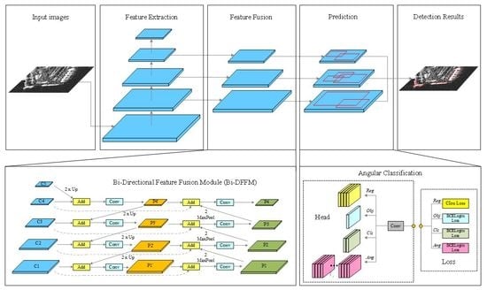
This paper proposes an arbitrary-oriented ship detector based on the YOLO detection framework using bi-directional feature fusion and angular classification. The overall scheme of the proposed method is shown in Figure 2.
As shown in Figure 2, we first send the preprocessed SAR image to Cross Stage Partial Networks (CSPDarknet53 [55]) for feature extraction, then five different feature maps (C1, C2, C3, C4, C5) can be obtained. In order to integrate shallow information into high-level features and achieve multiscale feature fusion at different resolutions more efficiently, we designed a bi-directional feature fusion module (Bi-DFFM). Based on the fused feature maps (P2, P3, P4), the bounding box (x, y, w, h), confidence scores (s), class (c) and angle category (Ac) of the targets are predicted at the improved head network. The predicted results are continuously optimized by iterating the new loss function. Finally, the final detection results are obtained via the modified rotated non-maximum suppression (R-NMS).
3.2. Random Rotation Mosaic Data Augmentation (RR-Mosaic)
To reduce the use of GPU and enrich the training dataset, Bochkovskiy et al. [55] proposed a new method of data augmentation named mosaic data augmentation. The specific implementation process can be summarized as follows: First, four pictures (f1, f2, f3, f4) are randomly selected from the training dataset; then, the selected pictures are randomly scaled and cut to obtain the processed images; finally, these processed pictures are randomly arranged and mosaiced to get the final expanded dataset (F1, F2, F3, F4). The mosaic data augmentation method can greatly enrich the training dataset, especially for small targets, and improve the robustness of the detection network. However, it can be found that the mosaic data augmentation method does not change the sample distribution on the original dataset but increases the imbalance of angle category. Specifically, for the proposed angular classification task, if there are many samples with angle () in the training dataset, then traditional mosaic data augmentation will increase the number of samples with angle (), thereby reducing the generalization performance of proposed model. To address this issue, we propose a new random rotation mosaic (RR-Mosaic) data augmentation method, as shown in Figure 3.
Unlike the conventional mosaic data augmentation method, the angle category is balanced by adding random rotation when processing the image. In our method, we first randomly select four pictures (f1, f2, f3, f4) from the overall training dataset, similar to the process described in the original mosaic method. After that, we randomly select four rotation angles () within the range of 0–180° and rotate these images according to the corresponding angle. At the same time, we transform the bounding box of all targets with the selected rotation angle to obtain the new labels. Then, we randomly flip, scale and transform the rotated image, finally obtaining the new training dataset by using the mosaic method. It can be found that the data augmentation method proposed in this paper not only increases the number of samples but also reduces the imbalance of angle categories (see Section 4 for more detailed experiment results).
3.3. Bi-Directional Feature Fusion Module (Bi-DFFM)
The conventional deep learning-based target detection algorithms, whether one-stage or two-stage, usually directly connect the head network with the last feature layer (generated by the backbone network) to predict the target position and category. However, it can be found that these conventional object detection algorithms cannot use a single feature map to effectively represent multi-scale objects at the same time. Therefore, object detection algorithms gradually developed to use different scales feature maps to predict the multi-scale objects. The feature pyramid network (FPN) [56] first proposed a top-down pathway to combine multiscale features. PANet [57] proposed an extra bottom-up path aggregation network based on FPN. ASFF [58] leveraged the attention mechanism to control the contribution value of different feature maps. NAS-FPN [59] proposed a merging cell to re-merge the features extracted from the backbone. Recursive-FPN [60] proposed a recursive feature fusion method. To optimize multi-scale feature fusion, Bi-FPN [61] proposed a bi-directional (top-down and bottom-up) fusion method. Inspired by Bi-FPN, we propose a novel bi-directional feature fusion module (Bi-DFFM) to efficiently aggregate features at different resolutions for ship detection in HR SAR images. Figure 4 illustrates the structure of the proposed Bi-DFFM. Proposed structure leverages weighted cross-scale connections to enable more high-level feature fusion without incurring extra computation burden. Meanwhile, this module can efficiently aggregate multi-scale features through bi-directional (top-down and bottom-up) information interaction, improving the detection performance of multi-scale ships.
As shown in Figure 4, the proposed Bi-DFFM takes level 1–5 features (extracted by backbone network) as input features , where denotes a feature level with a resolution of 1/2i of the input images. In our experiments, our input resolution is 512 × 512, so represents level 2 (512/22 = 128) feature with resolution 128 × 128, represents level 3 feature with resolution 64 × 64, represents level 4 feature with resolution 32 × 32, represents level 5 feature with resolution 16 × 16. To enhance the shallow information and high-level semantic information on the predicted features, we add a bi-directional (top-down and bottom-up) path to each level feature. In addition, we apply the fast normalized fusion method [61] to add additional weight for each input feature, reflecting the different contributions of different features. The Bi-DFFM aggregates multiscale features can be described as follows:
where P1′, P2′, P3′, P4′ denote the intermediate feature at level 1–level 4 on the top-down pathway. P1, P2, P3, P4 denote the corresponding output feature on the bottom-up pathway. () represents different learnable weights, is used to avoid numerical instability. represents a convolutional operation, and represent the upsampling and max-pooling operation.
3.4. Direction Prediction Based on Angular Classification
Most regression-based rotation detection methods leverage five tuples () to represent the oriented bounding box of a ship, where () is the coordinate of the center of the oriented bounding box, and are the width and length of the ship, respectively. The angle denotes the orientation angle, which is determined by the long side of the rectangle and x-axis, as shown in Figure 5. However, these methods essentially suffer the regression inconsistency issue near the boundary case, which makes the model’s loss value at the boundary suddenly increase. To avoid the inconsistency problem, we applied the Circular Smooth Label (CSL) [15] and Densely Coded Label (DCL) [16] to the head network to transform angular regression to angular classification. Specifically, CSL adopt the so-called Sparsely Coded Label (SCL) encoding technique to discretize the angle into a finite number of intervals. Note that the assigned label value for special angle is smooth with a certain tolerance, and then predicts a discrete angle by classification [15]. Unlike the CSL, DCL applied Binary Coded Label (BCL) and Gray Coded Label (GCL) to represent a larger range of values with less coding length, which effectively solve the problem of excessively long coding length in CSL [16].
Inspired by CSL-based and DCL-based detectors, we first convert the angle range from [−90, 0) to [0, 180), which can be summarized as the following equation:
where represents the original angle and represents changed angle which is used for angular classification.
Then, we treat degree per interval as an angle category. To obtain more robust angular prediction, we encode the angle category through different encoding methods, which can be formulated as
where AR denotes angle range (default is 180), NA represents the number of angle categories. Round function returns a numeric value that is the result of rounding to the specified number. and represent Circular Smooth Label and Densely Coded Label (see Equation (3) and Table 2), respectively. In the DCL-based method, only the number of categories is a power of 2 to ensure that each coding corresponds to a valid angle [16].
In this paper, we applied all angular classification methods to the designed detection framework. Furthermore, we conducted a series of comparative analyses to explore which angle representation method is more suitable for the direction prediction of ship targets in SAR images.
3.5. Multi-Task Loss Function
For the proposed arbitrary-oriented ship detection method, we add an angular classification prediction layer to the head network based on the YOLO framework, shown in Figure 2. Therefore, we add the angular classification loss to the original loss function.
where , , and denote the regression loss, confidence loss, classification loss and angular classification loss, respectively. The hyper-parameter , , and control the trade-off and are set to {1,1,1,1} by default.
The CIou_Loss [62] is adopted for , which is calculated as
where represents the thickness of predict layer (the default value is 3), represents the bounding boxes predicted by model, is the corresponding bounding boxes of ground truth, represents the number of ship targets. The , and are all calculated with binary cross-entropy (BCE) logits loss as follows:
where denotes the predicted offset vector, denotes the true vector, represents the width of feature maps in predict layer and represents the height of feature maps in predict layer. represents the predicted probability distribution of various classes, is the probability distribution of ground truth, is the number of ship types (the default value is 1). and denote the label and predict of angle with coding by CSL or DCL, respectively. represents the coding length of different angular classification methods. is defined as
where denotes the number of input vector, and represent corresponding predicted and true vector and is the Sigmoid function.
4. Experiments
Experimental dataset, implementation details and related evaluation metrics are first introduced in this section. Furthermore, extensive experiments are conducted to show the effectiveness and robustness of the proposed method.
4.1. Dataset Introduction
The dataset SSDD and large-scene HR SAR images from the GF-3 satellite are used to evaluate our proposed method. SSDD is the first published dataset for ship detection in SAR images. At present, there are two detection tasks for SSDD: horizontal bounding boxes (HBB) detection and oriented bounding boxes (OBB) detection. The SSDD dataset contains 1160 images and has 2456 ships ranging from the most miniature scale of 7 × 7 to the largest scale of 211 × 298. The polarization modes of these images include HH, HV, VV, and VH; resolutions also range from 1 to 15 m. The distributions of the sizes, aspect ratios, angle and corresponding error of the horizontal bounding boxes and oriented bounding boxes in SSDD are shown in Figure 6.
As shown in Figure 6d,e, there are large errors in the target information obtained based on HBB and OBB, which is also one of the motivations of this paper. In our experiments, 7/10 of the original images are randomly selected as the training set, 3/10 as the test set, as shown in Table 3. To make full use of the original size information, we adjust all images to 512 × 512 with padding operation. In addition, to verify the robustness of our model, we conduct experiments on large-scale HR SAR images obtained from the GF-3 satellite. GF-3 satellite has different imaging modes, such as the Spotlight (SL), Strip-Map (UFS), Fine Strip-Map 1 (FSI), Full Polarization 1 (QPSI), Full Polarization 2(QPSII) and Standard Strip (SS) modes. In our experiments, we mainly leverage HR SAR images from SL mode. We first divide the large-scale images into 512 × 512 sub-images with an overlap of 256 pixels, then we obtain about 14,879 patches and 24,849 ships with different sizes. After that, we divide all patches into training dataset and test dataset with the ratio of 7:3, as shown in Table 3. In the testing stage, all test patches are passed through a different model to get the predicted offsets, and the real coordinates in the large image are obtained by transforming the offsets according to corresponding overlap area. Figure 7 shows the large-scene HR SAR image and corresponding optical image. The distributions of the sizes, aspect ratios and angle of the horizontal bounding boxes in GF-3 dataset are shown in Figure 8.
4.2. Implementation Details
In this article, all experiments were implemented in PyTorch on a PC with Intel Core(TM) i7-10875H CPU @ 2.30GHz, NVIDIA RTX 2070 GPU. The PC operating system was Windows 10. We employ the Stochastic Gradient Descent (SGD) algorithm as the optimizer with 32 images per minibatch. The network weights are updated by using the initial learning rate of 1 × 10⁻², weight decay of 5 × 10⁻⁴ and momentum of 0.937. During the training phase, we use flip, rotation, random rotation, mosaic and RR-mosaic for data augmentation. During the test phase, we merge the detection results of all the slices to restore the detecting results on the large-scene SAR images. Finally, we apply rotated-Non-Maximum-Suppression (R-NMS) with an IoU threshold of 0.1 to discard repetitive detections, as shown in Figure 2. The computer and deep-learning environment configuration for our experiments is presented in Table 4.
4.3. Evaluation Metrics
We mainly leverage the precision, recall, average precision (AP), F1-score and precision-recall curve to evaluate the detection performance of different methods. Furthermore, we apply inference time per image to evaluate the detection efficiency of other methods. As for the algorithm complexity, we use the number of parameters and model size to evaluate different methods. The definition of precision and recall are as follows:
where TP (true positives), FP (false positives) and FN (false negative) refer to the number of correctly detected ships, false alarms and missing ships. F1 score combines the precision and recall as follows:
The AP is the average value of precisions based on different recalls, which is defined as
where P represents precision and R represents recall. The AP and F1-score metrics are applied to evaluate the comprehensive detection performance of the different models, and a larger value means a better detector performance. The PR curve reveals the relation between precision and recall, and the larger the area it covers, the better the detection result is.
4.4. Analysis of Results
To verify the effectiveness of each improvement proposed in this paper, we conducted a series of ablation experiments on the SSDD and GF-3 dataset. Furthermore, our method is compared with other methods to show the advantages of the proposed method in ship detection. Finally, we analyzed the detection results of our method in inshore, offshore and large-scenes SAR images, verifying the robustness of our model.
4.4.1. Effect of RR-Mosaic
Data augmentation methods can make a significant contribution to improving the performance of deep learning-based models and avoiding over-fitting effectively. However, for the angular classification-based method proposed in this paper, the conventional data augmentation methods such as flip, rotation and transform may enlarge the imbalance of angle category on original data, resulting in a decrease in detection performance. For this reason, we propose a new data augmentation method based on the classic mosaic method, named RR-Mosaic. To verify the effectiveness of the proposed method, we compare the detection performance of the different models under the same conditions. The angle distribution of different methods is shown in Figure 9, and corresponding detection results are shown in Table 5.
As shown in Table 5, compared with other data augmentation methods, the proposed RR-Mosaic can increase the randomness of angles in the augmented dataset and reduce the imbalance of angle category. In Table 5, almost scores of all indicators of RR-Mosaic are higher than those of Flip, Rotation, Random Rotation, Flip Mosaic and Rotation Mosaic. Especially, precision, AP and F1-score of RR-Mosaic are 1.36%, 0.84% and 0.061 higher than that of Flip Mosaic. Besides, the precision, recall, AP and F1-score of RR-Mosaic are 1.6%, 0.51%, 1.41% and 0.106 higher than that of Rotation Mosaic. It might be because of the increment of angle randomness by the proposed RR-Mosaic data augmentation method.
4.4.2. Effect of Angular Classification
Unlike the detection method with angular regression, the paper combines the YOLO detection framework with angular classification to predict the direction angle of the ship targets in HR SAR images. Figure 10 shows the detection results of the proposed method on the SSDD dataset. It can be seen that the proposed arbitrary-oriented ship detection framework based on angular classification can obtain the direction information of ship targets effectively and accurately. Compared with horizontal SAR ship detection methods, the bounding box generated by the proposed method best matches the real ship. For ships docked in the port intensively, our method can distinguish each target well by using the oriented bounding box. At the same time, the proposed method can accurately detect small-scale ship targets at open sea and obtain corresponding direction information, which further verifies the effectiveness of angular classification. Meanwhile, we compare the detection performance of our model using the two different angular classification methods with the original YOLOv5 detection model. Furthermore, comparison results of the methods without and with angular classification are listed in Table 6. As shown in Table 6, the proposed model with different angular classification methods shows a better performance than that without angular classification. Specifically, the precision, recall, AP and F1-score of BiFA-YOLO using CSL angular classification are 4.55%, 1.97%, 3.1% and 3.27% higher than that of YOLOv5, which further verifies that angular classification can effectively improve the model’s comprehensive detection performance. In addition, the angular classification method based on CSL is superior to the detection method based on DCL (using Gray Coded Label) in all indicators. Specifically, the AP value of the proposed method using CSL is 93.90%, which is 1.31% higher than that of proposed method using DCL. Furthermore, the F1 score of proposed method using CSL is 0.9441, which is higher than 0.9395 of proposed method using DCL. This may be because the ship targets in SAR images have significant characteristics of large aspect ratios. However, the DCL dense coding method is mainly used to improve the detection performance of square-like targets. Nevertheless, the experimental results shown in Figure 10 and Table 6 can thoroughly verify the impact of angular classification on detection performance.
4.4.3. Effect of Bi-Directional Feature Fusion Module
In this section, we compare the detection performance of the proposed model with different YOLOv5 models. The comparison of the detection results of the different models using CSL or DCL is presented in Table 7 and Table 8. Note that the inference time is measured at a resolution of 512 × 512 under the same experimental configuration. Furthermore, the number of parameters and the size of model are used to compare the complexity of different methods. The corresponding PR curves of different models are shown in Figure 11a,b. It can be seen from Table 7 and Table 8 that the detection performance of BiFA-YOLO is completely better than other models. For instance, the precision, recall, AP and F1 score of proposed BiFA-YOLO is 94.85%, 93.97%, 93.90% and 0.9441, which are 3.12%, 5.18%, 7.24% and 0.417 higher than that of YOLOv5s-CSL. Although our inference time is 13.3 ms (slower than 12.1 ms of YOLOv5s-CSL) and the parameters and model size are slightly larger than YOLOv5s-CSL, our method still has obvious advantages in detection performance. It might be because YOLOv5s has a simple network structure that cannot extract target feature information fully. Moreover, although the precision, recall, AP and F1 score of the proposed BiFA-YOLO are 0.25%, 0.31%, 1.17% and 0.019 slightly higher than that of YOLOv5x-CSL, the inference time of our model is 2.9 ms faster than that of YOLOv5x-CSL. In addition, the parameters and model size of the proposed model is 19.57 M and 39.4 M, which are obviously smaller than 85.50 M and 171.0 M of YOLOv5x-CSL. This may be because our B-DFFM leverages the most efficient cross-scale feature connection method, which does not require too many complicated calculations.
As shown in Figure 11 a,b, the purple curve of BiFA-YOLO is always above the other curves. It can be seen that whether the angular classification method is CSL or DCL, the performance of the four different YOLOv5 detection models is obviously lower than that of the proposed BiFA-YOLO model. This may be because the proposed Bi-DFMM can enrich the target feature information of different scales in the prediction layer.
4.4.4. Comparison of Inshore Scene and Offshore Scene
Table 9 shows the detection performance of the proposed model in inshore and offshore scenes on SSDD. It can be seen that the AP value of our model can exceed 90%, whether in the complex inshore scene or offshore scene. This shows that the model proposed in this paper can adapt to different scenarios. Specifically, our model’s precision, recall, AP and F1 score in the offshore scene are 96.16%, 95.55%, 94.81% and 0.9585, which are 3.35%, 3.95%, 3.66% and 0.365 higher than that in the inshore scene. This may be because there are more land background interference and many densely arranged ships in the inshore scene. In addition, it also shows that ship detection in the inshore scene is a more challenging task than that in offshore scene. Figure 12 shows the comparison of curves of different methods in inshore and offshore scene on SSDD. Figure 12a shows PR curves of different methods in inshore scene, and Figure 12b shows PR curves of different methods in offshore scene. It can be seen that the PR curve of our method is almost always higher than that of other methods in both inshore and offshore scene, indicating that the overall detection performance of the model is better than that of other methods.
Figure 13 shows the detection results of different methods in the inshore scene. It can be seen that there are a large number of densely arranged ship targets in the inshore scene. It is difficult for horizontal SAR ship detection methods to distinguish these ship targets with horizontal bounding boxes. In contrast, the arbitrary-oriented detection with the angular classification proposed in this paper can obtain the ship’s oriented bounding box to distinguish each ship. As shown in Figure 13, for the first condition of inshore scene (the first row to the second row of Figure 13), there is a missed ship in the detection result of YOLOv5s-CSL, YOLOv5s-DCL and YOLOv5m-DCL and a false alarm in the result of YOLOv5l-CSL and YOLOv5l-CSL. The other methods proposed in this paper can accurately detect the densely docked ships in the port. However, comparing the detection results of regions A and B, we can see that the oriented bounding boxes obtained by the proposed BiFA-YOLO method are more accurate and can better match these ships. For the second condition of the inshore scene (the third row to the fourth row of Figure 13), there are some false alarms in the detection result of YOLOv5s-CSL, YOLOv5l-CSL, YOLOv5m-DCL and YOLOv5l-DCL. Furthermore, there are some missed ships in all detection results, and this may be because the ship targets in area D are so closely docked, making it more difficult for the network to distinguish these ships. Similarly, comparing the detection results of regions C and D, it can be seen that the oriented bounding boxes obtained by the proposed BiFA-YOLO method are more accurate than other methods. This may be because Bi-DFFM can enhance the location information of the ship targets in the network prediction feature maps.
Figure 14 shows the detection results of different methods in the offshore scene. It can be seen that there are many dense small-scale ship targets in the first condition of offshore scene (the first row to the second row of Figure 14). Except for YOLOv5x-DCL and our BiFA-YOLO model, there are some false alarms in the detection results of other models. This may be because there are some false alarms that are very similar to the ships, making it more difficult for the network to identify effectively. However, due to the fusion of multi-scale features, our method can detect all ship targets and get accurate direction information. For the second condition of the offshore scene (the third row to the fourth row of Figure 14), there are three ship targets docked side by side, which is a challenge for ship detection. It can be seen that the BiFA-YOLO proposed in this paper can distinguish each ship and obtain the oriented bounding boxes of these ships accurately. However, there are some obviously missed ships and false alarms in the detection results of other methods.
4.4.5. Comparison with State of the Arts
In this section, the proposed BiFA-YOLO is compared with other existing arbitrary-oriented SAR ship detection methods, as shown in Table 10. It can be seen that the detection performance of the two-stage or multi-stage detection methods is generally better than that of the one-stage detection methods. However, the inference efficiency (obtained from corresponding literature) of one-stage detection methods is obviously faster than that of these two-stage or multi-stage detection methods. This may be because the two-stage or multi-stage detection network has a complex network structure and requires more computation. Recently, through the improvement of the network structure, some one-stage detection methods performed better in ship rotation detection have been proposed, such as R2FA-Det [48], R-RetinaNet [50], DRBox-v2 [51] and CSAP [54]. For example, the AP value of R-RetinaNet on the SSDD is 92.34%, and the inference time per image is only 46.5ms. The AP value of DRBox-v2 on the SSDD is 92.81%, and the inference time per image is 55.1ms. The AP value of the proposed method is 93.90%, which is 1.56 and 1.09% higher than that of R-RetinaNet and DRBox-v2, respectively. Furthermore, the inference time of our model is 13.3 ms, which is 33.2 and 41.8 ms faster than that of R-RetinaNet and DRBox-v2, respectively. Although the AP value of our method is 0.82% less than R2FA-Det, the inference time of our method is only about 1/5 of R2FA-Det. This may be because our method adopts an efficient feature fusion method and does not require too much computation.
Figure 15 shows some detection results of DRBox-v1 [51], SDOE [47], DRBox-v2 [51], the improved R-RetinaNet [50] and proposed BiFA-YOLO on SSDD. DRBox-v1 added a rotating frame to SSD. SDOE is built on the SSD framework with the attention module and angular regression. DRBox-v2 is an improved RBox-based target detection framework. The improved R-RetinaNet combined rotatable bounding box (RBox) with one-stage object detection framework based on RetinaNet. From the detection results of the first and second rows in Figure 15, it can be seen that our method shows better detection performance for multi-scale ship targets. This may be because other methods do not pay attention to the underlying information in the prediction layer, resulting in smaller targets being missed. For the complex inshore scenes (the third row to the sixth row of Figure 15), there are some false alarms in the detection results of other methods. In particular, some land areas in the inshore scene are mistakenly detected as targets by DRBox-v1. This phenomenon may be because Bi-DFFM can make full use of the characteristic information of different resolutions to improve classification performance and avoid the model from misclassifying the background as ship targets.
4.4.6. Validation on Large-Scene HR SAR Image
To fully verify the detection performance of the proposed method, we conducted some experiments on GF-3 large-scene SAR images, and some detection results are shown in Figure 16. Two specific areas marked with red rectangles are enlarged and shown in the lower part of Figure 16. The corresponding quantitative detection results are listed in the upper right corner of Figure 16. First, it can be seen that most of the ships at sea can be detected, and only two smaller ships (marked with a green ellipse) have been missed. This may be because the small ships are mistaken as a part of larger ships in the low-resolution feature map. Secondly, there are still some false alarms in the inshore scene. This problem is also one of the key problems that need to be solved in ship detection in SAR images. In addition, detection results on the enlarged areas indicates that our method can accurately obtain the direction information of ship targets. This may be because our method can provide the abundant location and semantic information, which is helpful for angular classification and location. In summary, the above experimental results show that the proposed method shows competitive detection performance on large scene images.
5. Discussion
As illustrated in Section 3.3, this paper proposes a novel bi-directional feature fusion module (Bi-DFFM) to aggregate features at different resolutions efficiently. To intuitively evaluate the effectiveness of Bi-DFFM, we visualized the intermediate feature maps of the feature pyramid with and without Bi-DFFM, as shown in Figure 17. Note that the brighter colors denote greater activation values in the visualization results. Figure 17a,c,e,g,i,k represent results without Bi-DFFM. Figure 17b,d,f,h,j,l represent results with Bi-DFFM. The two columns on the left in Figure 17 represent the visualization results of the inshore scene, and the two columns on the right in Figure 17 represent the visualization results of the offshore scene. It can be seen that whether in the inshore scene or the offshore scene, the position information of the ships in the feature maps after with Bi-DFMM is brighter and more accurate than that without Bi-DFMM. In addition, cross-scale joins in Bi-DFMM can combine semantic information of different scales to suppress background interference. This may be because the Bi-DFMM module can combine the underlying information from the high-resolution feature maps into the low-resolution feature maps.
In order to visually verify the effectiveness of the proposed BiFA-YOLO, we also visualized the intermediate feature maps of three scale prediction layers with and without Bi-DFFM, as shown in Figure 18. Note that x, y, w and h represent the feature maps for regressing the center coordinates, width and height of the ship’s bounding box in the head network. The four columns on the left in Figure 18 represent the visualization results of the inshore scene, and the four columns on the right in Figure 18 represent the visualization results of the offshore scene. Furthermore, the brighter colors denote greater activation values in the visualization results. Figure 18a,b,e,f,i,j represent results without Bi-DFFM. Figure 18c,d,g,h,k,l represent results with Bi-DFFM. It can be seen that active areas in the feature maps constructed with Bi-DFFM distribute more clearly than those without Bi-DFFM. Especially, the w and h feature maps in higher head show stronger position information, which is conducive to positioning these parallel ships. Meanwhile, the x and y feature maps constructed with Bi-DFFM can enrich the target position information and weaken the background clutters, improving the detection performance of multi-scale ship targets.
6. Conclusions
Aiming at accurately and efficiently detecting multi-scale, arbitrary-oriented and densely-distributed ship targets in HR SAR images, a novel YOLO-based method using bi-directional feature fusion and angular classification is proposed in this paper. Firstly, to improve the detection performance of multi-scale and densely distributed ships, we designed a novel bi-directional feature fusion module. This module can aggregate features at different resolutions by weighted cross-scale connections, which can enhance the information interaction in the feature maps with faster calculation efficiency. Secondly, the angular classification module instead of angular regression module is adopted to the YOLO detection framework for the first time. This module can obtain the direction information of ships with large aspect ratios more accurately without the problem of boundary discontinuity. In addition, a random rotation mosaic data augmentation method is proposed to address the angle imbalance caused by the conventional data augmentation method. Extensive experiments on SSDD indicated that the improvements proposed in this article can obtain an encouraging detection performance in terms of accuracy and speed. Especially in terms of detection speed, the inference time of our method is only 13.3 ms per 512 × 512 image, which is significantly faster than other methods. Furthermore, the experimental results on the large-scene HR SAR images confirmed the robustness and generalization ability of proposed method. On the whole, the BiFA-YOLO proposed in this paper adopts a new feature fusion and angular prediction method to detect ship targets in high-resolution SAR images. The experimental results prove that our method is superior to the existing arbitrary-oriented SAR ship detection methods in terms of detection time and performance and better meets the needs of actual marine ship detection system.
Author Contributions
Conceptualization, Z.S.; methodology, Z.S.; validation, Z.S.; formal analysis, Z.S. and Y.L.; investigation, Z.S. and Y.L.; resources, Z.S.; data curation, Z.S. and Y.L.; writing—original draft preparation, Z.S.; writing—review and editing, B.X., X.L., K.J.; visualization, Z.S.; supervision, K.J.; project administration, G.K.; funding acquisition, X.L. All authors have read and agreed to the published version of the manuscript.
Funding
This work was jointly supported by National Natural Science Foundation of China (62001480) and Hunan Provincial Natural Science Foundation of China (2021JJ40684).
Institutional Review Board Statement
Not applicable.
Informed Consent Statement
Not applicable.
Data Availability Statement
Not applicable.
Acknowledgments
The authors would like to thank the Chinese National Satellite Ocean Application Service for providing the data used in this article. Meanwhile, the authors would also like to thank the pioneer researchers in SAR ship detection and other related fields.
Conflicts of Interest
The authors declare no conflict of interest.
References
- Lang, H.; Xi, Y.; Zhang, X. Ship Detection in High-Resolution SAR Images by Clustering Spatially Enhanced Pixel Descriptor. IEEE Trans. Geosci. Remote Sens. 2019, 57, 5407–5423. [Google Scholar] [CrossRef]
- Leng, X.; Ji, K.; Kuang, G. Radio Frequency Interference Detection and Localization in Sentinel-1 Images. IEEE Trans. Geosci. Remote Sens. 2021, 1–12. [Google Scholar] [CrossRef]
- Zhang, P.; Luo, H.; Ju, M.; He, M.; Chang, Z.; Hui, B. Brain-Inspired Fast Saliency-Based Filtering Algorithm for Ship Detection in High-Resolution SAR Images. IEEE Trans. Geosci. Remote Sens. 2021, 1–9. [Google Scholar] [CrossRef]
- Zhang, L.; Leng, X.; Feng, S.; Ma, X.; Ji, K.; Kuang., G.; Liu, L. Domain Knowledge Powered Two-Stream Deep Network for Few-Shot SAR Vehicle Recognition. IEEE Trans. Geosci. Remote Sens. 2021, 1–15. [Google Scholar] [CrossRef]
- Wang, X.; Chen, C.; Pan, Z.; Pan, Z. Fast and Automatic Ship Detection for SAR Imagery Based on Multiscale Contrast Measure. IEEE Geosci. Remote Sens. Lett. 2019, 16, 1834–1838. [Google Scholar] [CrossRef]
- Yang, M.; Guo, C. Ship Detection in SAR Images Based on Lognormal ρ-Metric. IEEE Geosci. Remote Sens. Lett. 2018, 15, 1372–1376. [Google Scholar] [CrossRef]
- Ao, W.; Xu, F.; Li, Y.; Wang, H. Detection and Discrimination of Ship Targets in Complex Background from Spaceborne ALOS-2 SAR Images. IEEE J. Sel. Top. Appl. Earth Obs. Remote Sens. 2018, 11, 536–550. [Google Scholar] [CrossRef]
- Guo, H.; Yang, X.; Wang, N.; Gao, X. A CenterNet++ model for ship detection in SAR images. Pattern Recognit. 2021, 112, 107787. [Google Scholar] [CrossRef]
- Liang, Y.; Sun, K.; Zeng, Y.; Li, G.; Xing, M. An Adaptive Hierarchical Detection Method for Ship Targets in High-Resolution SAR Images. Remote Sens. 2020, 12, 303. [Google Scholar] [CrossRef] [Green Version]
- Leng, X.; Ji, K.; Xiong, B.; Kuang, G. Complex Signal Kurtosis—Indicator of Ship Target Signature in SAR Images. IEEE Trans. Geosci. Remote Sens. 2021. [Google Scholar] [CrossRef]
- Liu, T.; Yang, Z.; Yang, J.; Gao, G. CFAR Ship Detection Methods Using Compact Polarimetric SAR in a K-Wishart Distribution. IEEE J. Sel. Top. Appl. Earth Obs. Remote Sens. 2019, 12, 3737–3745. [Google Scholar] [CrossRef]
- Gao, G.; Shi, G. CFAR Ship Detection in Nonhomogeneous Sea Clutter Using Polarimetric SAR Data Based on the Notch Filter. IEEE Trans. Geosci. Remote Sens. 2017, 55, 4811–4824. [Google Scholar] [CrossRef]
- Dai, H.; Du, L.; Wang, Y.; Wang, Z. A Modified CFAR Algorithm Based on Object Proposals for Ship Target Detection in SAR Images. IEEE Geosci. Remote Sens. Lett. 2016, 13, 1925–1929. [Google Scholar] [CrossRef]
- Leng, X.; Ji, K.; Yang, K.; Zou, H. A Bilateral CFAR Algorithm for Ship Detection in SAR Images. IEEE Geosci. Remote Sens. Lett. 2015, 12, 1536–1540. [Google Scholar] [CrossRef]
- Yang, X.; Yan, J.; He, T. Arbitrary-Oriented Object Detection with Circular Smooth Label. In Proceedings of the European Conference on Computer Vision (ECCV), Glasgow, UK, 23–28 August 2020; pp. 677–694. [Google Scholar]
- Yang, X.; Hou, L.; Zhou, Y.; Wang, W.; Yan, J. Dense Label Encoding for Boundary Discontinuity Free Rotation Detection. arXiv 2020, arXiv:2011.09670. [Google Scholar]
- Li, J.; Qu, C.; Shao, J. Ship detection in SAR images based on an improved faster R-CNN. In Proceedings of the BIGSARDATA, Beijing, China, 13–14 November 2017; pp. 1–6. [Google Scholar]
- Ren, S.; He, K.; Girshick, R.; Sun, J. Faster R-CNN: Towards real-time object detection with region proposal networks. IEEE Trans. Pattern Anal. Mach. Intell. 2017, 39, 1137–1149. [Google Scholar] [CrossRef] [Green Version]
- Lin, Z.; Ji, K.; Leng, X.; Kuang, G. Squeeze and Excitation Rank Faster R-CNN for Ship Detection in SAR Images. IEEE Geosci. Remote Sens. Lett. 2018, 16, 751–755. [Google Scholar] [CrossRef]
- Deng, Z.; Sun, H.; Zhou, S.; Zhao, J. Learning Deep Ship Detector in SAR Images from Scratch. IEEE Trans. Geosci. Remote Sens. 2019, 57, 4021–4039. [Google Scholar] [CrossRef]
- Wang, Y.; Wang, C.; Zhang, H.; Dong, Y.; Wei, S. A SAR Dataset of Ship Detection for Deep Learning under Complex Backgrounds. Remote Sens. 2019, 11, 765. [Google Scholar] [CrossRef] [Green Version]
- Liu, W.; Anguelov, D.; Erhan, D.; Szegedy, C.; Reed, S. SSD: Single shot multibox detector. arXiv 2015, arXiv:1512.02325. [Google Scholar]
- Lin, T.; Goyal, P.; Girshick, R.; He, K.; Dollar, P. Focal loss for dense object detection. arXiv 2017, arXiv:1708.02002. [Google Scholar]
- Ai, J.; Tian, R.; Luo, Q.; Jin, J.; Tang, B. Multi-Scale Rotation-Invariant Haar-Like Feature Integrated CNN-Based Ship Detection Algorithm of Multiple-Target Environment in SAR Imagery. IEEE Trans. Geosci. Remote Sens. 2019, 57, 10070–10087. [Google Scholar] [CrossRef]
- Wei, S.; Su, H.; Ming, J.; Wang, C.; Yan, M.; Kumar, D.; Shi, J.; Zhang, X. Precise and Robust Ship Detection for High-Resolution SAR Imagery Based on HR-SDNet. Remote Sens. 2020, 12, 167. [Google Scholar] [CrossRef] [Green Version]
- Cui, Z.; Li, Q.; Cao, Z.; Liu, N. Dense Attention Pyramid Networks for Multi-Scale Ship Detection in SAR Images. IEEE Trans. Geosci. Remote Sens. 2019, 57, 8983–8997. [Google Scholar] [CrossRef]
- Wang, Y.; Wang, C.; Zhang, H.; Dong, Y.; Wei, S. Automatic Ship Detection Based on RetinaNet Using Multi-Resolution Gaofen-3 Imagery. Remote Sens. 2019, 11, 531. [Google Scholar] [CrossRef] [Green Version]
- Fu, J.; Sun, X.; Wang, Z.; Fu, K. An Anchor-Free Method Based on Feature Balancing and Refinement Network for Multiscale Ship Detection in SAR Images. IEEE Trans. Geosci. Remote Sens. 2021, 59, 1331–1344. [Google Scholar] [CrossRef]
- Gao, F.; He, Y.; Wang, J.; Hussain, A.; Zhou, H. Anchor-free Convolutional Network with Dense Attention Feature Aggregation for Ship Detection in SAR Images. Remote Sens. 2020, 12, 2619. [Google Scholar] [CrossRef]
- Cui, Z.; Wang, X.; Liu, N.; Cao, Z. Ship Detection in Large-Scale SAR Images Via Spatial Shuffle-Group Enhance Attention. IEEE Trans. Geosci. Remote Sens. 2021, 59, 379–391. [Google Scholar] [CrossRef]
- Zhou, X.; Wang, D.; Krähenbühl, P. Objects as points. arXiv 2019, arXiv:1904.07850. [Google Scholar]
- Zhao, Y.; Zhao, L.; Xiong, B.; Kuang, G. Attention Receptive Pyramid Network for Ship Detection in SAR Images. IEEE J. Sel. Top. Appl. Earth Obs. Remote Sens. 2020, 13, 2738–2756. [Google Scholar] [CrossRef]
- Chen, S.; Zhan, R.; Wang, W.; Zhang, J. Learning Slimming SAR Ship Object Detector Through Network Pruning and Knowledge Distillation. IEEE J. Sel. Top. Appl. Earth Obs. Remote Sens. 2021, 14, 1267–1282. [Google Scholar] [CrossRef]
- Yu, L.; Wu, H.; Zhong, Z.; Zheng, L.; Deng, Q.; Hu, H. TWC-Net: A SAR Ship Detection Using Two-Way Convolution and Multiscale Feature Mapping. Remote Sens. 2021, 12, 2558. [Google Scholar] [CrossRef]
- Zhang, T.; Zhang, X. ShipDeNet-20: An Only 20 Convolution Layers and <1-MB Lightweight SAR Ship Detector. IEEE Geosci. Remote Sens. Lett. 2021, 18, 1234–1238. [Google Scholar] [CrossRef]
- Geng, X.; Shi, L.; Yang, J.; Li, P.; Zhao, L.; Sun, W.; Zhao, J. Ship Detection and Feature Visualization Analysis Based on Lightweight CNN in VH and VV Polarization Images. Remote Sens. 2021, 13, 1184. [Google Scholar] [CrossRef]
- Sun, Z.; Dai, M.; Leng, X.; Lei, Y.; Xiong, B.; Ji, K.; Kuang, G. An Anchor-Free Detection Method for Ship Targets in High-Resolution SAR Images. IEEE J. Sel. Top. Appl. Earth Obs. Remote Sens. 2021, 14, 7788–7816. [Google Scholar] [CrossRef]
- Bao, W.; Huang, M.; Zhang, Y.; Xu, Y.; Liu, X.; Xiang, X. Boosting ship detection in SAR images with complementary pretraining techniques. IEEE J. Sel. Top. Appl. Earth Obs. Remote Sens. 2021, 14, 8941–8954. [Google Scholar] [CrossRef]
- Zhang, T.; Zhang, X.; Ke, X. Quad-FPN: A Novel Quad Feature Pyramid Network for SAR Ship Detection. Remote Sens. 2021, 13, 2771. [Google Scholar] [CrossRef]
- Hong, Z.; Yang, T.; Tong, X.; Zhang, Y.; Jiang, S.; Zhou, R.; Han, Y.; Wang, J.; Yang, S.; Liu, S. Multi-Scale Ship Detection from SAR and Optical Imagery Via a More Accurate YOLOv3. IEEE J. Sel. Top. Appl. Earth Obs. Remote Sens. 2021, 14, 6083–6101. [Google Scholar] [CrossRef]
- Zhang, X.; Huo, C.; Xu, N.; Jiang, H.; Cao, Y.; Ni, L.; Pan, C. Multitask Learning for Ship Detection from Synthetic Aperture Radar Images. IEEE J. Sel. Top. Appl. Earth Obs. Remote Sens. 2021, 14, 8048–8062. [Google Scholar] [CrossRef]
- Li, D.; Liang, Q.; Liu, H.; Liu, Q.; Liu, H.; Liao, G. A Novel Multidimensional Domain Deep Learning Network for SAR Ship Detection. IEEE Trans. Geosci. Remote Sens. 2021. [Google Scholar] [CrossRef]
- Jiang, J.; Fu, X.; Qin, R.; Wang, X.; Ma, Z. High-Speed Lightweight Ship Detection Algorithm Based on YOLO-V4 for Three-Channels RGB SAR Image. Remote Sens. 2021, 13, 1909. [Google Scholar] [CrossRef]
- Tang, G.; Zhuge, Y.; Claramunt, C.; Men, S. N-YOLO: A SAR Ship Detection Using Noise-Classifying and Complete-Target Extraction. Remote Sens. 2021, 13, 871. [Google Scholar] [CrossRef]
- Xu, P.; Li, Q.; Zhang, B.; Wu, F.; Zhao, K.; Du, X.; Yang, C.; Zhong, R. On-Board Real-Time Ship Detection in HISEA-1 SAR Images Based on CFAR and Lightweight Deep Learning. Remote Sens. 2021, 13, 1995. [Google Scholar] [CrossRef]
- Wu, Z.; Hou, B.; Ren, B.; Ren, Z.; Wang, S.; Jiao, L. A Deep Detection Network Based on Interaction of Instance Segmentation and Object Detection for SAR Images. Remote Sens. 2021, 13, 2582. [Google Scholar] [CrossRef]
- Wang, J.; Lu, C.; Jiang, W. Simultaneous Ship Detection and Orientation Estimation in SAR Images Based on Attention Module and Angle Regression. Sensors 2018, 18, 2851. [Google Scholar] [CrossRef] [Green Version]
- Chen, S.; Zhang, J.; Zhan, R. R2FA-Det: Delving into High-Quality Rotatable Boxes for Ship Detection in SAR Images. Remote Sens. 2020, 12, 2031. [Google Scholar] [CrossRef]
- Pan, Z.; Yang, R.; Zhang, Z. MSR2N: Multi-Stage Rotational Region Based Network for Arbitrary-Oriented Ship Detection in SAR Images. Sensors 2020, 20, 2340. [Google Scholar] [CrossRef] [PubMed] [Green Version]
- Yang, R.; Pan, Z.; Jia, X.; Zhang, L.; Deng, Y. A Novel CNN-Based Detector for Ship Detection Based on Rotatable Bounding Box in SAR Images. IEEE J. Sel. Top. Appl. Earth Obs. Remote Sens. 2021, 14, 1938–1958. [Google Scholar] [CrossRef]
- An, Q.; Pan, Z.; Liu, L.; You, H. DRBox-v2: An improved detector with rotatable boxes for target detection in SAR images. IEEE Trans. Geosci. Remote Sens. 2019, 57, 8333–8349. [Google Scholar] [CrossRef]
- Yang, R.; Wang, G.; Pan, Z.; Lu, H.; Zhang, H.; Jia, X. A Novel False Alarm Suppression Method for CNN-Based SAR Ship Detector. IEEE Geosci. Remote Sens. Lett. 2021, 18, 1401–1405. [Google Scholar] [CrossRef]
- Chen, C.; He, C.; Hu, C.; Pei, H.; Jiao, L. MSARN: A Deep Neural Network Based on an Adaptive Recalibration Mechanism for Multiscale and Arbitrary-Oriented SAR Ship Detection. IEEE Access 2019, 7, 159262–159283. [Google Scholar] [CrossRef]
- An, Q.; Pan, Z.; You, H.; Hu, Y. Transitive Transfer Learning-Based Anchor Free Rotatable Detector for SAR Target Detection with Few Samples. IEEE Access 2021, 9, 24011–24025. [Google Scholar] [CrossRef]
- Bochkovskiy, A.; Wang, C.; Liao, H.M. YOLOv4: Optimal Speed and Accuracy of Object Detection. arXiv 2020, arXiv:2004.10934. [Google Scholar]
- Lin, T.; Dollár, P.; Girshick, R.; He, K.; Hariharan, B.; Belongie, S. Feature pyramid networks for object detection. arXiv 2016, arXiv:1612.03144. [Google Scholar]
- Liu, S.; Qi, L.; Qin, H.; Shi, J.; Jia, J. Path aggregation network for instance segmentation. arXiv 2018, arXiv:1803.01534. [Google Scholar]
- Liu, S.; Huang, D.; Wang, Y. Learning Spatial Fusion for Single-Shot Object Detection. arXiv 2019, arXiv:1911.09516. [Google Scholar]
- Ghiasi, G.; Lin, T.Y.; Pang, R.; Le, Q.V. NAS-FPN: Learning Scalable Feature Pyramid Architecture for Object Detection. arXiv 2019, arXiv:1911.09516. [Google Scholar]
- Qiao, S.; Chen, L.; Yuille, A. DetectoRS: Detecting Objects with Recursive Feature Pyramid and Switchable Atrous Convolution. arXiv 2020, arXiv:2006.02334. [Google Scholar]
- Tan, M.; Pang, R.; Le, Q.V. EfficientDet: Scalable and Efficient Object Detection. arXiv 2019, arXiv:1911.09070. [Google Scholar]
- Zheng, Z.; Wang, P.; Liu, W.; Li, J.; Ren, D. Distance-IoU Loss: Faster and Better Learning for Bounding Box Regression. arXiv 2019, arXiv:1911.08287. [Google Scholar] [CrossRef]
- Yang, X.; Yang, J.; Yan, J.; Zhang, Y.; Zhang, T.; Guo, Z.; Xian, S.; Fu, K. SCRDet: Towards More Robust Detection for Small, Cluttered and Rotated Objects. arXiv 2018, arXiv:1811.07126. [Google Scholar]
Figure 2.
The overall scheme of the proposed method.

Figure 3.
Random rotation mosaic (RR-Mosaic) data augmentation.

Figure 4.
Structure of Bi-DFFM.

Figure 5.
The oriented bounding box (OBB) of ships in SAR images, where is determined by the long side of the rectangle and x-axis. (a) belongs to [−90, 0). (b) belongs to [0, 90).
Figure 5.
The oriented bounding box (OBB) of ships in SAR images, where is determined by the long side of the rectangle and x-axis. (a) belongs to [−90, 0). (b) belongs to [0, 90).

Figure 6.
The distributions of the sizes, aspect ratios, angle and corresponding error of the horizontal bounding boxes and oriented bounding boxes in SSDD. (a) Distributions of the bounding boxes’ length in SSDD. (b) Distributions of the bounding boxes’ width in SSDD. (c) Distributions of the bounding boxes’ sizes in SSDD. (d) Distributions of the bounding boxes’ aspect ratios in SSDD. (e) Distributions of corresponding errors of the HBB and OBB in SSDD. (f) Distributions of the oriented bounding boxes’ angle in SSDD.

Figure 7.
The large-scene images. (a) GF-3 HR SAR image. (b) Corresponding optical image.

Figure 8.
The distributions of the sizes, aspect ratios and angle of the oriented bounding boxes in GF-3 dataset. (a) Distributions of the bounding boxes’ length in GF-3 dataset. (b) Distributions of the bounding boxes’ width in GF-3 dataset. (c) Distributions of the bounding boxes’ aspect ratios in GF-3 dataset. (d) Distributions of the oriented bounding boxes’ angle in GF-3 dataset.

Figure 9.
Distributions of the angle on SSDD with different data augmentation methods. (a) Flip. (b) Rotation. (c) Radom Rotation. (d) Flip Mosaic. (e) Rotation Mosaic. (f) RR-Mosaic.
Figure 9.
Distributions of the angle on SSDD with different data augmentation methods. (a) Flip. (b) Rotation. (c) Radom Rotation. (d) Flip Mosaic. (e) Rotation Mosaic. (f) RR-Mosaic.

Figure 10.
Experimental results on SSDD. The blue number represents the number of detected ships.

Figure 11.
Precision-Recall (PR) curves of different models on SSDD. (a) PR curves of YOLOv5s-CSL, YOLOv5m-CSL, YOLOv5l-CSL, YOLOv5x-CSL and BiFA-YOLO. (b) PR curves of YOLOv5s-DCL, YOLOv5m- DCL, YOLOv5l-DCL, YOLOv5x-DCL and BiFA-YOLO.
Figure 11.
Precision-Recall (PR) curves of different models on SSDD. (a) PR curves of YOLOv5s-CSL, YOLOv5m-CSL, YOLOv5l-CSL, YOLOv5x-CSL and BiFA-YOLO. (b) PR curves of YOLOv5s-DCL, YOLOv5m- DCL, YOLOv5l-DCL, YOLOv5x-DCL and BiFA-YOLO.

Figure 12.
Comparison of curves of different methods in inshore and offshore scene on SSDD. (a) PR curves of different methods in inshore scene. (b) PR curves of different methods in offshore scene.
Figure 12.
Comparison of curves of different methods in inshore and offshore scene on SSDD. (a) PR curves of different methods in inshore scene. (b) PR curves of different methods in offshore scene.

Figure 13.
Detection results of different methods in inshore scene. (a,k) ground-truths. (b,l) results of YOLOv5s-CSL. (c,m) results of YOLOv5m-CSL. (d,n) results of YOLOv5l-CSL. (e,o) results of YOLOv5x-CSL. (f,p) results of YOLOv5s-DCL. (g,q) results of YOLOv5m-DCL. (h,r) results of YOLOv5l-DCL. (i,s) results of YOLOv5x-DCL. (j,t) results of BiFA-YOLO. Note that the red boxes represent true positive targets, the yellow ellipses represent false positive targets and the green ellipses represent missed targets.

Figure 14.
Detection results of different methods in offshore scene. (a,k) ground-truths. (b,l) results of YOLOv5s-CSL. (c,m) results of YOLOv5m-CSL. (d,n) results of YOLOv5l-CSL. (e,o) results of YOLOv5x-CSL. (f,p) results of YOLOv5s-DCL. (g,q) results of YOLOv5m-DCL. (h,r) results of YOLOv5l-DCL. (i,s) results of YOLOv5x-DCL. (j,t) results of BiFA-YOLO. Note that the red boxes represent true positive targets, the yellow ellipses represent false positive targets and the green ellipses represent missed targets.

Figure 15.
Detection results of different CNN-based methods on SSDD. (a,g,m) ground-truths. (b,h,n) results of DRBox-v1. (c,i,o) results of SDOE. (d,j,p) results of DRBox-v2. (e,k,q) results of improved R-RetinaNet. (f,l,r) results of proposed BiFA-YOLO. Note that the red boxes represent true positive targets, the yellow ellipses represent false positive targets and the green ellipses represent missed targets; the blue number represents the number of detected ships.

Figure 16.
Detection results in large-scene SAR image. Note that the red boxes represent true positive targets, the yellow ellipses represent false positive targets and the green ellipses represent missed targets; and the blue number represents the number of detected ships.
Figure 16.
Detection results in large-scene SAR image. Note that the red boxes represent true positive targets, the yellow ellipses represent false positive targets and the green ellipses represent missed targets; and the blue number represents the number of detected ships.

Figure 17.
Feature map visualization results of feature pyramid with and without Bi-DFFM. (a,c,e,g,i,k) represent results without Bi-DFFM. (b,d,f,h,j,l) represent results with Bi-DFFM.
Figure 17.
Feature map visualization results of feature pyramid with and without Bi-DFFM. (a,c,e,g,i,k) represent results without Bi-DFFM. (b,d,f,h,j,l) represent results with Bi-DFFM.

Figure 18.
Feature map visualization results of three-scale prediction layers with and without Bi-DFFM. (a,b,e,f,i,j) represent results without Bi-DFFM. (c,d,g,h,k,l) represent results with Bi-DFFM.
Figure 18.
Feature map visualization results of three-scale prediction layers with and without Bi-DFFM. (a,b,e,f,i,j) represent results without Bi-DFFM. (c,d,g,h,k,l) represent results with Bi-DFFM.


Table 1.
The division of angle category.
| Range | Categories | |
|---|---|---|
| 0–180° | 1 | 180 |
| 0–180° | 2 | 90 |
| 0–90° | 1 | 90 |
| 0–90° | 2 | 45 |
Table 2.
The binary coded label and gray coded label corresponding to the angle categories.
| Angle Category | 1 | 45 | 90 | 135 | 179 |
|---|---|---|---|---|---|
| Binary Coded Label | 00000001 | 01000000 | 10000000 | 11000000 | 11111111 |
| Gray Coded Label | 00000001 | 01100000 | 11000000 | 10100000 | 10000000 |
Table 3.
Division of different datasets.
| Dataset | Training | Test | ALL |
|---|---|---|---|
| SSDD | 812 | 348 | 1160 |
| GF-3 Dataset | 10,150 | 4729 | 14,879 |
Table 4.
Experimental environment.
| Project | Model/Parameter |
|---|---|
| CPU | Intel i7-10875H |
| RAM | 32 GB |
| GPU | NVIDIA RTX 2070 |
| System | windows 10 |
| Code | python3.8 |
| Framework | CUDA10.1/cudnn7.6.5/torch 1.6 |
Table 5.
Detection results with different data augmentation methods.
| Method | Precision (%) | Recall (%) | AP (%) | F1 |
|---|---|---|---|---|
| Flip | 93.84 | 93.02 | 92.23 | 0.9343 |
| Rotation | 93.65 | 93.23 | 92.25 | 0.9344 |
| Random Rotation | 94.80 | 93.33 | 92.72 | 0.9408 |
| Flip Mosaic | 93.49 | 94.13 | 93.06 | 0.9380 |
| Rotation Mosaic | 93.25 | 93.46 | 92.49 | 0.9335 |
| RR-Mosaic | 94.85 | 93.97 | 93.90 | 0.9441 |
Table 6.
Comparison of the methods without and with angular classification.
| Method | Precision (%) | Recall (%) | AP (%) | F1 |
|---|---|---|---|---|
| YOLOv5 | 90.30 | 92.00 | 90.80 | 0.9114 |
| BiFA-YOLO + CSL | 94.85 | 93.97 | 93.90 | 0.9441 |
| BiFA-YOLO + DCL | 94.25 | 93.66 | 92.59 | 0.9395 |
Table 7.
Comparison of different models using the CSL on SSDD.
| Method | Precision (%) | Recall (%) | AP (%) | F1 | Time (ms) | Params (M) | Model (M) |
|---|---|---|---|---|---|---|---|
| YOLOv5s-CSL | 91.73 | 88.79 | 86.66 | 0.9024 | 12.1 | 7.38 | 14.9 |
| YOLOv5m-CSL | 91.86 | 93.02 | 90.78 | 0.9244 | 13.2 | 21.19 | 42.6 |
| YOLOv5l-CSL | 93.03 | 93.23 | 92.25 | 0.9313 | 13.8 | 46.13 | 92.6 |
| YOLOv5x-CSL | 94.60 | 93.66 | 92.73 | 94.22 | 16.2 | 85.50 | 171.0 |
| BiFA-YOLO | 94.85 | 93.97 | 93.90 | 0.9441 | 13.3 | 19.57 | 39.4 |
Table 8.
Comparison of different models using the DCL on SSDD.
| Method | Precision (%) | Recall (%) | AP (%) | F1 | Time (ms) | Params (M) | Model (M) |
|---|---|---|---|---|---|---|---|
| YOLOv5s-DCL | 91.93 | 88.69 | 85.75 | 0.9028 | 12.0 | 6.94 | 14.0 |
| YOLOv5m-DCL | 92.20 | 92.49 | 89.69 | 0.9235 | 13.6 | 20.53 | 41.3 |
| YOLOv5l-DCL | 92.23 | 92.92 | 90.63 | 0.9257 | 15.4 | 45.24 | 90.8 |
| YOLOv5x-DCL | 94.69 | 92.39 | 91.29 | 0.9353 | 15.7 | 84.39 | 169.0 |
| BiFA-YOLO | 94.85 | 93.97 | 93.90 | 0.9441 | 13.3 | 19.57 | 39.4 |
Table 9.
Detection results of the proposed method in inshore and offshore scene on SSDD.
| Scene | Precision (%) | Recall (%) | AP (%) | F1 |
|---|---|---|---|---|
| Inshore | 92.81 | 91.60 | 91.15 | 0.9220 |
| Offshore | 96.16 | 95.55 | 94.81 | 0.9585 |
Table 10.
Detection results of different CNN-based methods on SSDD.
| Method | Bounding Box | Framework | AP (%) | Time (ms) |
|---|---|---|---|---|
| R-FPN [49] | Oriented | Two-Stages | 84.38 | - |
| R-Faster-RCNN [49] | Oriented | Two-Stages | 82.22 | - |
| RRPN [53] | Oriented | Two-Stages | 74.82 | 316.0 |
| R2CNN [53] | Oriented | Two-Stages | 80.26 | 210.8 |
| R-DFPN [53] | Oriented | Two-Stages | 83.44 | 370.5 |
| MSR2N [49] | Oriented | Two-Stages | 93.93 | 103.3 |
| SCRDet [63] | Oriented | Two-Stages | 92.04 | 120.8 |
| Cascade RCNN [48] | Oriented | Multi-Stages | 88.45 | 357.6 |
| R-YOLOv3 [53] | Oriented | One-Stage | 73.15 | 34.2 |
| R- Attention-ResNet [53] | Oriented | One-Stage | 76.40 | 39.6 |
| R-RetinaNet [50] | Oriented | One-Stage | 92.34 | 46.5 |
| R2FA-Det [48] | Oriented | One-Stage | 94.72 | 63.2 |
| DRBox-v1 [51] | Oriented | One-Stage | 86.41 | - |
| DRBox-v2 [51] | Oriented | One-Stage | 92.81 | 55.1 |
| MSARN [53] | Oriented | One-Stage | 76.24 | 35.4 |
| CSAP [54] | Oriented | One-Stage | 90.75 | - |
| SDOE [47] | Oriented | One-Stage | 84.20 | 25.0 |
| BiFA-YOLO | Oriented | One-Stage | 93.90 | 13.3 |
Publisher’s Note: MDPI stays neutral with regard to jurisdictional claims in published maps and institutional affiliations. |
© 2021 by the authors. Licensee MDPI, Basel, Switzerland. This article is an open access article distributed under the terms and conditions of the Creative Commons Attribution (CC BY) license (https://creativecommons.org/licenses/by/4.0/).
Share and Cite
MDPI and ACS Style
Sun, Z.; Leng, X.; Lei, Y.; Xiong, B.; Ji, K.; Kuang, G. BiFA-YOLO: A Novel YOLO-Based Method for Arbitrary-Oriented Ship Detection in High-Resolution SAR Images. Remote Sens. 2021, 13, 4209. https://doi.org/10.3390/rs13214209
AMA Style
Sun Z, Leng X, Lei Y, Xiong B, Ji K, Kuang G. BiFA-YOLO: A Novel YOLO-Based Method for Arbitrary-Oriented Ship Detection in High-Resolution SAR Images. Remote Sensing. 2021; 13(21):4209. https://doi.org/10.3390/rs13214209
Chicago/Turabian StyleSun, Zhongzhen, Xiangguang Leng, Yu Lei, Boli Xiong, Kefeng Ji, and Gangyao Kuang. 2021. "BiFA-YOLO: A Novel YOLO-Based Method for Arbitrary-Oriented Ship Detection in High-Resolution SAR Images" Remote Sensing 13, no. 21: 4209. https://doi.org/10.3390/rs13214209
Note that from the first issue of 2016, this journal uses article numbers instead of page numbers. See further details here.