A Novel Bayesian Super-Resolution Method for Radar Forward-Looking Imaging Based on Markov Random Field Model

Abstract

Super-resolution technology is considered as an efficient approach to promote the image quality of forward-looking imaging radar. However, super-resolution technology is inherently an ill-conditioned issue, whose solution is quite susceptible to noise. Bayesian method can efficiently alleviate this issue through utilizing prior knowledge of the imaging process, in which the scene prior information plays a pretty significant role in ensuring the imaging accuracy. In this paper, we proposed a novel Bayesian super-resolution method on the basis of Markov random field (MRF) model. Compared with the traditional super-resolution method which is focused on one-dimensional (1-D) echo processing, the MRF model adopted in this study strives to exploit the two-dimensional (2-D) prior information of the scene. By using the MRF model, the 2-D spatial structural characteristics of the imaging scene can be well described and utilized by the nth-order neighborhood system. Then, the imaging objective function can be constructed through the maximum a posterior (MAP) framework. Finally, an accelerated iterative threshold/shrinkage method is utilized to cope with the objective function. Validation experiments using both synthetic echo and measured data are designed, and results demonstrate that the new MAP-MRF method exceeds other benchmarking approaches in terms of artifacts suppression and contour recovery.

1. Introduction

Radar forward-looking imaging has extensive applications in military and civil territories, for instance, in the automatic landing of aircraft, material airdrops, topographic mapping, etc. [1,2]. However, the conventional monostatic synthetic aperture radar (SAR) and Doppler beam sharpening (DBS) techniques cannot be utilized to image the forward area due to the difficulty in acquiring an effective Doppler bandwidth [3,4].

An effective strategy for radar forward-looking imaging is acquiring the real-aperture scanning image first. Then, signal processing techniques are utilized on the real-aperture image to improve the azimuth resolution. One typical method used is monopulse imaging technology (MIT), which employs the monopulse angle measurement technology to ameliorate the visual quality of the real-aperture image [5,6]. However, targets located in the same radar beam cannot be discriminated by the MIT; thus, no actual resolution improvement can be acquired.

Recently, angular super-resolution technology has aroused researchers’ interest owing to its low hardware complexity and high efficiency in enhancing the angular resolution [7,8,9]. The fact that the azimuth echo of a scanning radar is the convolution of the antenna pattern and the scattering coefficient is taken into account by this technology. Hence, deconvolution should be an efficient technology for improving the angular resolution. Theoretically, the resolution could be infinitely improved under the ideal conditions, i.e, without noise in the echo. Nevertheless, the deconvolution approach is inherently an ill-conditioned issue and the solution is extremely unstable when the echo is contaminated [10].

Multiple methods have been proposed for addressing the noise-sensitive problem of deconvolution. These methods can be classified as regularization technology and Bayesian technology. In regularization technology, the ill-conditioned issue is transformed into a constrained least squares estimation with Euclidean norm theory. One of the most representative regularization approaches is the Tikhonov method, which can reduce the noise sensitivity by adopting an L2-norm constraint at the cost of a reduction in resolution [11,12]. In Reference [13], L1-norm regularization combined with the truncated singular value decomposition (TSVD) algorithm is conducted for radar forward imaging. Even a high super-resolution ratio can be achieved for sparse targets, and the scene contour can be destroyed simultaneously. In addition, the utilization of total variation (TV) has been introduced prior to this for radar forward imaging in some studies [14,15,16], and the results have verified its recoverability for contour information.

The Bayesian method provides a systematic and consistent way to deal with the ill-conditioned problem through statistical optimization. In Reference [17], the noise and targets are modeled as the Poisson distribution, and the angular resolution is enhanced at least four times under a low SNR condition. Zha et al. [18] consider the noise as a mixed distribution, i.e., Gaussian distribution and Poisson distribution, while Laplace distribution is used to model the targets. The proposed method is able to distinguish strong targets more efficiently due to its utilization of sparse prior information. However, since the Poisson distribution is more suitable for describing photon behavior, these methods are not compatible for radar imaging. As a matter of fact, the probability distribution of baseband radar signal is supposed to be determined by I/Q two-way noise distribution due to the coherence of the radar imaging system. In our previous study, we proposed an I/Q channel-based maximum likelihood approach, with the results exhibiting a strong competence of anti-noise [19]. After that, based on noise modeling, a maximum a posteriori method that models the targets as a combined distribution, i.e., Gaussian distribution and Laplace distribution, is proposed [20]. The experiment results demonstrate that the proposed method performs more effectively in eliminating spurious targets and strengthening the algorithm robustness in low-SNR conditions.

Unfortunately, in the state-of-the-art research on this topic, only one-dimensional (1-D) prior information has been utilized. In imaging tasks, the structure of an imaging scene is two-dimensional (2-D), and every pixel is assumed to be determined by the neighborhood around it. Although the TV prior can describe the 2-D spatial relationship of the pixels, the relevant studies have only used TV prior within one distance cell, thus confining its two-dimensional representation capacity. Therefore, the utilization of scene prior information needs to be further developed.

In this paper, a novel super-resolution imaging method based on the Bayesian method is proposed. The reason why we chose to use the Bayesian method instead of the regularization method is that statistical optimization approaches are able to interpret prior information more flexibly for both the noise and targets. Through the use of the Maximum a posteriori (MAP) framework of the Bayesian method, the noise and targets can be modeled, respectively, in view of a statistical perspective. Therefore, the noise is firstly modeled through I/Q channel, thus allowing an accurate likelihood function to be obtained. Differently from the traditional real-aperture imaging method, Markov random field (MRF) is adopted in this paper. Compared with the 1-D modeling method, the MRF can describe the spatial continuity and structural features more efficiently for its ability in modeling the conditional distribution of each pixel about the adjacent pixels. By selecting an appropriate neighborhood system for MRF and employing the MAP framework, the structural characteristics and interacting features can be well described and absorbed into the imaging objective function, thus greatly facilitating the improvement of the resolution and image contour recovery. At last, an accelerated iterative threshold/shrinking (IST) method is utilized to cope with the objective function for its superiority in fast convergence and noise resistance.

The framework of this article is structured as follows: Firstly, the super-resolution imaging mold of real-aperture scanning radar (RASR) is described in Section 2. In Section 3, the Bayesian framework and likelihood function are derived first; then, the MRF is introduced, and the Huber MRF is adopted to formulate the imaging objective function; afterwards, the derivation of the proposed MAP-MRF method is presented. Section 4 illustrates the results of the numerical simulation and a real data experiment. A discussion of the results is demonstrated in Section 5. Section 6 provides a brief conclusion.

2. Super-Resolution Echo Model for RASR

Figure 1 illustrates an imaging sketch of the RASR in which the aircraft flies along the y-axis at a constant speed of v. The radar beam scans anticlockwise with the rotational rate $\omega$, transmitting and receiving LFM signals. We suppose that there is a target P in the irradiation area and that its initial distance to the radar is $r_0$. According to the geometry relationship in Figure 1, the range history of target P can be stated as:

$$r_P\left(t\right)=\sqrt{r_0^2+{\left(vt\right)}^2-2r_{0}vtcos{\theta }_{0}cos\phi },$$

(1)

where t denotes the azimuth–time variable, ${\theta }_0$ is the initial azimuth angle of target P, and $\phi$ is the incident angle. Since the required imaging time is relatively short owing to the rapid scanning velocity and small imaging area, $r_P\left(t\right)$ can be roughly expanded into [21]

$$r_P\left(t\right)\approx r_0-vtcos{\theta }_{0}cos\phi .$$

(2)

In addition, since the imaging area is less than ${10}^{\circ }$, $cos{\theta }_0$ can be approximated as 1. Thus, $r_P\left(t\right)$ can be further deduced as:

$$r_P\left(t\right)\approx r_0-vtcos\phi .$$

(3)

We assume that the transmitted signal $s_{out}\left(\tau \right)$ is:

$$s_{out}\left(\tau \right)=rect\left(\frac{\tau }{T_r}\right)exp\left\{j2\pi f_c\tau \right\}exp\left\{j2\pi K{\tau }^2\right\},$$

(4)

where $\tau$ denotes the range–time variable, $T_r$ denotes the signal width, $f_c$ denotes the carrier frequency, K is the frequency modulation rate of LFM, and $rect\left(·\right)$ is defined as:

$$rect\left(\frac{\tau }{T_r}\right)=\left\{\begin{array}{c}1\tau \le \left|\frac{T_r}{2}\right|\hfill \\ 0,other\hfill \end{array}.\right.$$

(5)

After quadrature demodulation, the baseband complex signal is obtained as

$$s_P(\tau ,t)={\sigma }_{0}h(t-t_0)exp\left\{j\pi Kr{\left(\tau -2r_P\left(t\right)/c\right)}^2\right\}exp\left\{-j\frac{4\pi }{\lambda }{r}_P\left(t\right)\right\},$$

(6)

where ${\sigma }_0$ is the scattering coefficient, which is assumed to be constant during the scanning process, $h\left(t\right)$ is the radiation pattern of the antenna, and $t_0$ is the center time, while scanning P, c denotes the light speed, and $\lambda$ denotes the wavelength. By using the approximated range history in Equation (6), the echo after pulse compression can be stated as:

$$s_P(\tau ,t)={\sigma }_{0}h(t-t_0)exp\left\{j\pi Kr{\left(\tau -2\left(r_0-vtcos\phi \right)/c\right)}^2\right\}exp\left\{-j\frac{4\pi }{\lambda }\left(r_0-vtcos\phi \right)\right\}.$$

(7)

For analyzing the azimuth signal, the obtained echo can be preprocessed by pulse compression and range migration correction [21]. After that, $s_P(\tau ,t)$ is rewritten as

$${\tilde{s}}_P(\tau ,t)={\sigma }_{0}h(t-t_0)\mathrm{sinc}\left(\tau -\frac{2r_0}{c}\right)exp\left\{-j\frac{4\pi }{\lambda }\left(r_0-vtcos\phi \right)\right\}.$$

(8)

In order to analyze the echo in the space variable space, we translate the time variables on the basis of $t=\left(\theta -{\theta }_a\right)/\omega$ and $\tau =2r/c$, where $\theta$ is the azimuth angle variable, and r is the range variable. Then, Equation (8) can be converted to:

$$s_P(r,\theta )={\sigma }_{0}h\left(\theta -{\theta }_0\right)\mathrm{sinc}\left[\frac{2B}{c}\left(r-r_0\right)\right]exp\left\{-j\frac{4\pi }{\lambda }\left(r_0-v\frac{\theta -{\theta }_a}{\omega }cos\phi \right)\right\}.$$

(9)

Therefore, the echo of the area targets with scattering coefficient $\sigma (r,\theta )$ is obtained by integrating Equation (9):

$$s_{\Omega }(r,\theta )=\int \int \tilde{\sigma }(\overline{r},\overline{\theta })h\left(\theta -\overline{\theta }\right)\mathrm{sinc}\left\{\frac{2B}{c}\left(r-\overline{r}\right)\right\}\mathrm{d}\overline{r}\mathrm{d}\overline{\theta }exp\left(j\phi \left(\theta \right)\right),$$

(10)

where $\overline{r}$ and $\overline{\theta }$ are the integral variables in angular direction and range direction, respectively; $\tilde{\sigma }(\overline{r},\overline{\theta })$ equals $\sigma (\overline{r},\overline{\theta })\exp \left(\frac{4\pi }{\lambda }\overline{r}\right)$, which denotes the phase-weighted scattering function; $\phi \left(\theta \right)$ equals $\frac{4\pi }{\lambda }v\frac{\theta -{\theta }_a}{\omega }cos\phi$, which is independent of the integral variable. Providing that the azimuth echo is extracted, a more concise azimuth convolution model can be obtained:

$$s_A\left(\theta \right)=\sigma \left(\theta \right)\otimes h\left(\theta \right),$$

(11)

where ⊗ denotes convolution operation, and $s_A\left(\theta \right)$ is the amplitude of the azimuth echo. Considering the analysis simplicity and system noise, the super-resolution convolution model (11) can be further discretized by a matrix vector form:

$$s=H\sigma +n,$$

(12)

where $s={\left[s_1,\dots ,s_N\right]}^T$ is the measured echo, N denotes the sampling points, $\sigma ={\left[{\sigma }_1,\dots ,{\sigma }_N\right]}^T$ denotes the targets distribution to be estimated, $n={\left[n_1,\dots ,n_N\right]}^T$ represents the system noise, and H is the convolution matrix that is cyclically formulated to facilitate matrix vector multiplication through fast Fourier transform (FFT).

$$H=\left[h\left({\theta }_1\right),h\left({\theta }_2\right),\dots ,h\left({\theta }_N\right)\right]={\left[\begin{array}{ccccccc}{h}_{1,1}& & & & h_{L,N-L+2}& \cdots & h_{2,N}\\ h_{2,1}& h_{1,2}& & & & \ddots & h_{3,N}\\ ⋮& & \ddots & & & & ⋮\\ h_{L,1}& & & & & & \\ & \ddots & & & & & \\ & & \ddots & & & & \\ & & & h_{L,N-L+1}& \cdots & h_{2,N-1}& h_{1,N}\end{array}\right]}_{N\times N}.$$

(13)

According to Equation (12), the azimuth resolution has been seriously worsened owing to the convolution impact of the scanning beam. Based on the convolution model, the deconvolution technique can be adopted to promote the azimuth resolution. Furthermore, to relief the noise sensitivity of the deconvolution and utilize the structural prior information more comprehensively, the MRF is employed to model the targets in this paper.

3. Methodology

3.1. Bayesian Framework

The Bayesian technique is a fundamental theory in estimation and decision-making. Based on Bayesian theory, the forward-looking imaging problem can be formulated from a probabilistic perspective. To be more specific, in the Bayesian framework, all the unknown and observed variables are treated as stochastic variables. Then, the deconvolution imaging problem is converted to maximize the posterior probability function of the targets. To begin, the posterior probability function can be stated as:

$$P\left(\sigma \left|s\right.\right)=\frac{P\left(s\left|\sigma \right.\right)P\left(\sigma \right)}{P\left(s\right)},$$

(14)

where $P\left(s\left|\sigma \right.\right)$ is the likelihood function, and $P\left(\sigma \right)$ and $P\left(s\right)$ are the probability distributions of $\sigma$ and s, respectively. Since $P\left(s\right)$ in Equation (14) is a constant for a fixed s, maximizing $P\left(\sigma \left|s\right.\right)$ is equivalent to maximizing the joint distribution:

$$\widehat{\sigma }=\underset{\sigma }{argmax}P\left(s\left|\sigma \right.\right)P\left(\sigma \right).$$

(15)

For the ease of derivation, the log function is utilized to separate the multiplication terms in Equation (15):

$$\widehat{\sigma }=\underset{\sigma }{argmax}lnP\left(s\left|\sigma \right.\right)+lnP\left(\sigma \right).$$

(16)

For a given $\sigma$, the likelihood function is determined by the probability distribution of the noise. In a radar system, the noise is generated by electrons’ thermal motion and subjected to a Gaussian distribution. After quadrature demodulation, the radar echo is transformed to a complex signal composed of I/Q two-way signals. Meanwhile, the echo of the I/Q channel is also contaminated by the Gaussian noise:

$$\left\{\begin{array}{c}I:s_I=H\sigma cos\phi +n_I\hfill \\ Q:s_Q=H\sigma sin\phi +n_Q\hfill \end{array}.\right.$$

(17)

Thus, according to Equation (17), the amplitude probability function of the measured complex data is mainly determined by the probability distribution of the I/Q channel noise. Since this paper is mainly concerned with the prior modeling of targets, the derivation of the likelihood function is skipped and given directly here. The detailed derivation process can be found in our previous article [19].

$$lnP\left(s_A\left|\sigma \right.\right)=\sum _{i=1}^{N}ln{J}_0\left(\frac{s_i{\left(H\sigma \right)}_i}{{\rho }^2}\right)-\sum _{i=1}^N\frac{{\left({\left(H\sigma \right)}_i\right)}^2}{2{\rho }^2},$$

(18)

where $s_A$ is the amplitude of the demodulated echo, ${\left(·\right)}_i$ is the $i-th$ element of the vector in the bracket, $\rho$ is the standard deviation of the noise probability distribution, and $J_0\left(·\right)$ denotes the zero-order Bessel function.

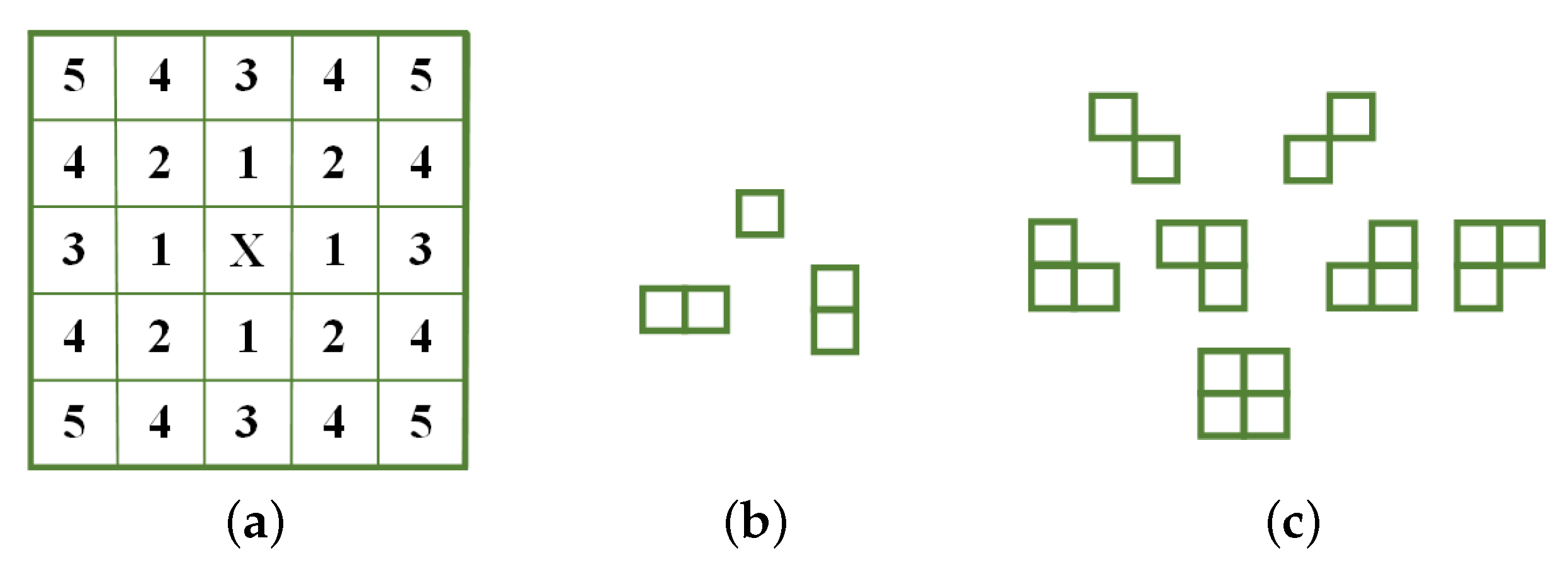
3.2. Markov Radom Field Model

Spatial structure information takes on a significant character in the imaging process. Within the structure of an image, there is a certain correlation and regularity between the pixels, and the brightness value of a pixel is assumed to be closely related to other nearby pixels. Markov random field can effectively model this spatial structure relationship and describe the local statistical characteristics of a pixel and the pixels around [22,23,24]. Thus, the MRF is utilized to model the priori information of the targets of this paper.

To describe the mutual impact between one pixel and the others, the concept of clique ℏ is introduced. For image description, cliques ℏ represent the basic structure of an image texture, as is roughly demonstrated in Figure 2, in which Figure 2a displays the fifth-order neighborhood system, and Figure 2b,c display the cliques for the first-order neighborhood and second-order neighborhood, respectively. As can be observed from Figure 2, these basic cliques can comprehensively describe the two-dimensional spatial structure characteristics in the neighborhood system.

Based on the definitions, the random field defined in MRF can be acquired according to the Markov–Gibbs equivalence, which can be written as:

$$p\left(\sigma \right)=\frac{1}{Z}exp\left[-U\left(\sigma \right)\right],$$

(19)

where Z is a normalizing constant, and $U\left(\sigma \right)$ denotes the energy function, which is defined as:

$$U\left(\sigma \right)\stackrel{}{=}\sum _{\hslash \in \Omega }{V}_{\hslash }\left(\sigma \right),$$

(20)

where $V_{\hslash }\left(\sigma \right)$ is the potential function associated with the clique ℏ, and $\Omega$ is the set of all possible structures of ℏ. The energy function relies on specific images and the pixel values contained in the cliques. In this paper, the Huber–Markov prior model is chosen as the potential function for its competence in protecting the edge information [25], which is stated as:

$$p\left(\sigma \right)=\frac{1}{Z}exp\left\{-\frac{1}{\tau }\sum _{\hslash \in \Omega }{\rho }_T\left(d_{\hslash }^n\left(\sigma \right)\right)\right\},$$

(21)

where ${\rho }_T\left(·\right)$ denotes the Huber function, $\tau$ is a temperature coefficient, and $d_{\hslash }^n$ denotes the derivative operation, which is defined using second-order derivatives as

$$\begin{array}{c}{d}_{i,j}^0={\sigma }_{i,j+1}-2{\sigma }_{i,j}+{\sigma }_{i,j-1}\hfill \\ d_{i,j}^1=\frac{1}{2}({\sigma }_{i-1,j+1}-2{\sigma }_{i,j}+{\sigma }_{i+1,j-1})\hfill \\ d_{i,j}^2={\sigma }_{i-1,j}-2{\sigma }_{i,j}+{\sigma }_{i+1,j}\hfill \\ d_{i,j}^3={\sigma }_{i-1,j-1}-2{\sigma }_{i,j}+{\sigma }_{i+,j+1}\hfill \end{array}.$$

(22)

The Huber function is given by:

$${\rho }_T\left(x\right)=\left\{\begin{array}{c}{x}^2\left|x\right|\le \Lambda \hfill \\ 2\Lambda \left|x\right|-{\Lambda }^2\left|x\right|>\Lambda \hfill \end{array}\right..$$

(23)

The threshold $\Lambda$ will punish the change in gray level in the image space. To smooth the small-scale noise, a square penalty is applied to the area with a flat gray level change, i.e., ($\left|x\right|\le \Lambda$), while the linear penalty is applied to the image edge with strong gray level change, i.e., ($\left|x\right|>\Lambda$). $\Lambda$ is regarded as the dividing point between high-frequency components and low-frequency components, which can be determined by the formula:

$$\Lambda ={\left\{Sort\left(\left|\sum _{n=0}^3{d}_{i,j}^n\left({\sigma }_{i,j}\right)\right|,i=2,\cdots ,N-1;j=2,\cdots ,M-1\right)\right\}}_{(N-2)\times (M-2)\times ƛ},$$

(24)

where ${\sigma }_{i,j}$ denotes the value of $\sigma$ located at column i and row j; $Sort\left(·\right)$ denotes the sort in descending order for second-order derivative and taking the value at position $(N-2)\times (M-2)\times ƛ$; M and N are the sampling points in terms of azimuth and distance, respectively; and $ƛ$ is the proportion of high-frequency components determined in advance. Since we normally suppose that the medium- and low-frequency components in the image are higher than the high-frequency components, $ƛ$ can be taken as a value between 0 and 1/2.

Through substituting Equations (18) and (21) into Equation (16), the final objective function for MAP-MRF can be obtained. The derivation is illustrated in Appendix A.

$$\widehat{\sigma }=\left\{\begin{array}{c}\underset{\sigma }{argmin}{F}_1\left(\sigma \right)=\underset{\sigma }{argmin}\left\{\sum _{i=1}^{N}ln{J}_0\left(\frac{s_i{\left(H\sigma \right)}_i}{{\rho }^2}\right)-\sum _{i=1}^N\frac{{\left({\left(H\sigma \right)}_i\right)}^2}{2{\rho }^2}+\lambda \sum _{i=2}^{N-1}\sum _{j=2}^{M-1}\sum _{n=0}^3{\left(d_{i,j}^n\left({\sigma }_{i,j}\right)\right)}^2\right\}\left|\sum _{n=0}^3{d}_{i,j}^n\left({\sigma }_{i,j}\right)\right|\le \Lambda \hfill \\ \underset{\sigma }{argmin}{F}_2\left(\sigma \right)=\underset{\sigma }{argmin}\left\{\sum _{i=1}^{N}ln{J}_0\left(\frac{s_i{\left(H\sigma \right)}_i}{{\rho }^2}\right)-\sum _{i=1}^N\frac{{\left({\left(H\sigma \right)}_i\right)}^2}{2{\rho }^2}+\lambda \sum _{i=2}^{N-1}\sum _{j=2}^{M-1}\sum _{n=0}^3\left(2\Lambda \left|d_{i,j}^n\left({\sigma }_{i,j}\right)\right|-{\Lambda }^2\right)\right\}\left|\sum _{n=0}^3{d}_{i,j}^n\left({\sigma }_{i,j}\right)\right|>\Lambda \hfill \end{array}.\right.$$

(25)

Equation (25) demonstrates the objective function obtained. Parameter $\lambda$ controls the relative weight of the prior term and can be determined through the L-curve method [26]. Then, the forward-looking super-resolution imaging problem of RASA can be transformed into the optimal solution of Equation (25).

3.3. Solution to the Objective Function

Equation (25) is a non-linear optimization problem. To acquire the minimum value of objective function (25), the gradient-based approach can be adopted, where the derivative information is used to search for the optimal value. However, the absolute term in $F_2\left(\sigma \right)$ is non-differentiable, thus the gradient-based method no longer being in force. Fortunately, through introducing a minuscule parameter $\epsilon$, $F_2\left(\sigma \right)$ can be made differentiable.

$$F_2\left(\sigma \right)=\sum _{i=1}^{N}ln{J}_0\left(\frac{s_i{\left(H\sigma \right)}_i}{{\rho }^2}\right)-\sum _{i=1}^N\frac{{\left({\left(H\sigma \right)}_i\right)}^2}{2{\rho }^2}+\lambda \sum _{i=2}^{N-1}\sum _{j=2}^{M-1}\sum _{n=0}^3\left(2\Lambda \left(\sqrt{\left({\left(d_{i,j}^n\left({\sigma }_{i,j}\right)\right)}^2+\epsilon \right)}\right)-{\Lambda }^2\right).$$

(26)

Normally, the $\epsilon$ can be taken as ${10}^{-10}$. Then, we take the derivative of function $F_1\left(\sigma \right)$ and $F_2\left(\sigma \right)$ with respect to $\sigma$. The gradient of the two objective functions can be calculated as:

$$\begin{array}{c}\nabla F_1\left(\sigma \right)=\frac{1}{{\rho }^2}{H}^T\left[\frac{J_1\left(\frac{s_i{\left(H\sigma \right)}_i}{{\rho }^2}\right)}{J_0\left(\frac{s_i{\left(H\sigma \right)}_i}{{\rho }^2}\right)}\odot s\right]-\frac{1}{{\rho }^2}{H}^{T}H\sigma -\lambda \sum _{n=0}^3{d}_{i,j}^n\left(\sigma \right)\hfill \\ \nabla F_2\left(\sigma \right)=\frac{1}{{\rho }^2}{H}^T\left[\frac{J_1\left(\frac{s_i{\left(H\sigma \right)}_i}{{\rho }^2}\right)}{J_0\left(\frac{s_i{\left(H\sigma \right)}_i}{{\rho }^2}\right)}\odot s\right]-\frac{1}{{\rho }^2}{H}^{T}H\sigma -\lambda \sum _{n=0}^{3}diag\left\{{\left({\left|d_{i,j}^n\left({\sigma }_{i,j}\right)\right|}^2+\epsilon \right)}^{-\frac{1}{2}}\right\}{d}_{i,j}^n\left(\sigma \right)\hfill \end{array},$$

(27)

where $diag\left(·\right)$ is a diagonal matrix. Thus, the optimal value of $\sigma$ can be obtained by iterative searching along the gradient direction.

$${\sigma }_{k+1}=\left\{\begin{array}{c}{\sigma }_k-\beta \nabla F_1\left({\sigma }_k\right)\left|\sum _{n=0}^3{d}_{i,j}^n\left({\sigma }_k\right)\right|\le \Lambda \hfill \\ {\sigma }_k-\beta \nabla F_2\left({\sigma }_k\right)\left|\sum _{n=0}^3{d}_{i,j}^n\left({\sigma }_k\right)\right|>\Lambda \hfill \end{array},\right.$$

(28)

where ${\sigma }_{k+1}$ and ${\sigma }_k$ are the $\left(k+1\right)-th$ and $k-th$ iterative results, respectively; $\beta$ is the step size, which is confined within $2/∥H^{T}H∥$ to guarantee the convergence of the iteration. However, this simple iterative method converges slowly and is still sensitive to noise. Therefore, an acceleration strategy with an iterative shrinkage/thresholding (IST) solution is employed to solve the objective function to facilitate the engineering implementation [27]. This accelerated IST method can not only effectively reduce the impact of noise through the IST operation, but also quickly obtain the optimal solution. The basic iterative steps of IST can be obtained based on Equation (28), which is:

$${\sigma }_{k+1}=\left\{\begin{array}{c}{\psi }_1\left({\sigma }_k\right)={\Re }_{\delta }\left\{{\sigma }_k-\beta \nabla F_1\left({\sigma }_k\right)\right\}\left|\sum _{n=0}^3{d}_{i,j}^n\left({\sigma }_k\right)\right|\le \Lambda \hfill \\ {\psi }_2\left({\sigma }_k\right)={\Re }_{\delta }\left\{{\sigma }_k-\beta \nabla F_2\left({\sigma }_k\right)\right\}\left|\sum _{n=0}^3{d}_{i,j}^n\left({\sigma }_k\right)\right|>\Lambda \hfill \end{array},\right.$$

(29)

where ${\mathrm{R}}^N\to R^N$: ${\mathrm{R}}^N\to R^N$ is the shrinkage-thresholding operation

$${\Re }_{\delta }\left(\sigma \right)=\left\{\begin{array}{c}0,\left|\sigma \right|\le \delta \hfill \\ \sigma -\delta \mathrm{sgn}\left(\sigma \right),otherwise\hfill \end{array},\right.$$

(30)

where $\delta$ can be determined according to the noise level. When it is difficult to estimate the noise, we simply set $\delta$ as zero to ensure the non-negativity of the results. Afterwards, to improve the convergence speed, a vector extrapolation strategy is use to accelerate the iterative process. That is, before each iteration, the first two iterations are used to predict the next iteration, which is:

$$y_{k+1}={\sigma }_k+{\alpha }_k\left({\sigma }_k-{\sigma }_{k-1}\right).$$

(31)

The prediction step ${\alpha }_k$ is determined by the direction similarity of the first two iterations

$${\alpha }_k=\frac{{\sum g_k·g}_{k-1}}{{\sum g_{k-1}·g}_{k-1}}0<{\alpha }_k<1,$$

(32)

where $g_k$ is the direction vector $g_k={\sigma }_k-{\sigma }_{k-1}$. Then, the iteration operation is conducted on $y_{k+1}$. Through utilizing the prediction result, the iterative result can progress much faster along the convergence path.

Since the convolution kernel in this paper is formulated as a cyclic-convolution matrix, the matrix-vector multiplication can be transformed into point-multiplication in the frequency domain using FFT. Thus, the calculation complexity of MAP-MRF in one complete iteration can be calculated as $4Nlog2N+30N$ complex multiplications and $7Nlog2N+26N$ complex additions. Additionally, since the acceleration strategy only needs linear operation, it will not burden the calculation while improving the convergence speed.

In conclusion, the implementation steps of the MAP-MRF method are given as follows:

Input: the parameters $\beta$, $\delta$, and $\lambda$

Initial Step: Give s for the initial iteration ${\sigma }_0$.

Calculate the threshold $\Lambda$ according to Equation (24)

Then: Calculate the first two iterative results ${\sigma }_1$ and ${\sigma }_2$ with the iteration

Equation (29) and the first two iterative vectors $g_1={\sigma }_1-{\sigma }_0$ and $g_2={\sigma }_2-{\sigma }_1$

Repeat

Compute the extrapolation step size ${\alpha }_k$ according to Equation (32)

Compute the prediction result $y_{k+1}$ according to Equation (31)

If $\left|\sum _{n=0}^3{d}_{i,j}^n\left({\sigma }_k\right)\right|\le \Lambda$, calculate the iterative point ${\sigma }_{k+1}$ through the upper

iteration formula Equation (28): ${\sigma }_{k+1}={\psi }_1\left(y_{k+1}\right)$

If $\left|\sum _{n=0}^3{d}_{i,j}^n\left({\sigma }_k\right)\right|>\Lambda$, calculate the iterative point ${\sigma }_{k+1}$ through the lower

iteration formula Equation (28): ${\sigma }_{k+1}={\psi }_2\left(y_{k+1}\right)$

Update the iterative vector $g_{k+1}={\sigma }_{k+1}-{\sigma }_k$

Update the threshold according to Equation (24)

Until (convergence)

Export the final value ${\sigma }_{k+1}$

4. Numerical Results

The numerical results based on both the simulation experiment and measured echo are presented in this section to validate the efficiency of MAP-MRF super-resolution methods for angular super-resolution imaging.

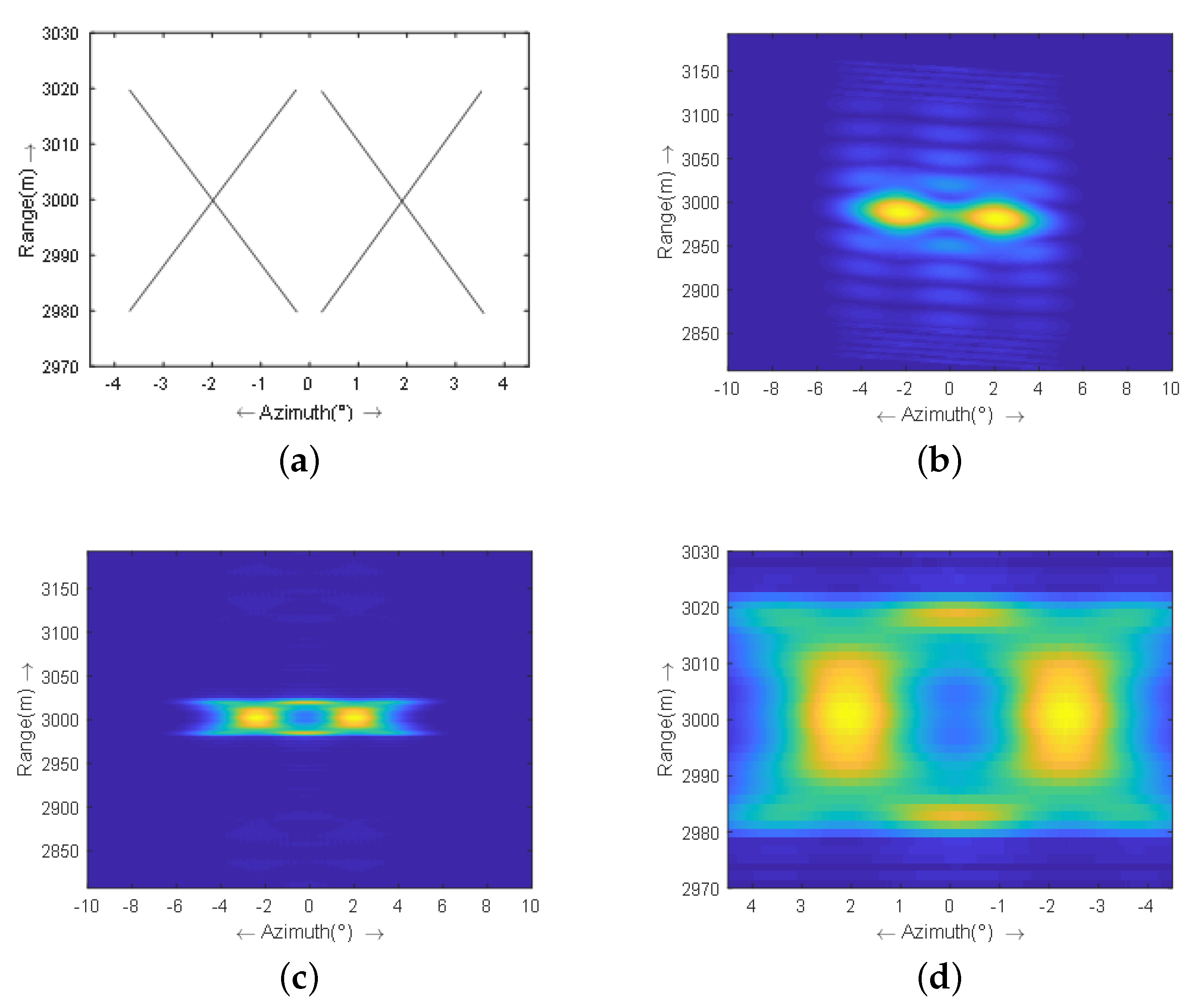
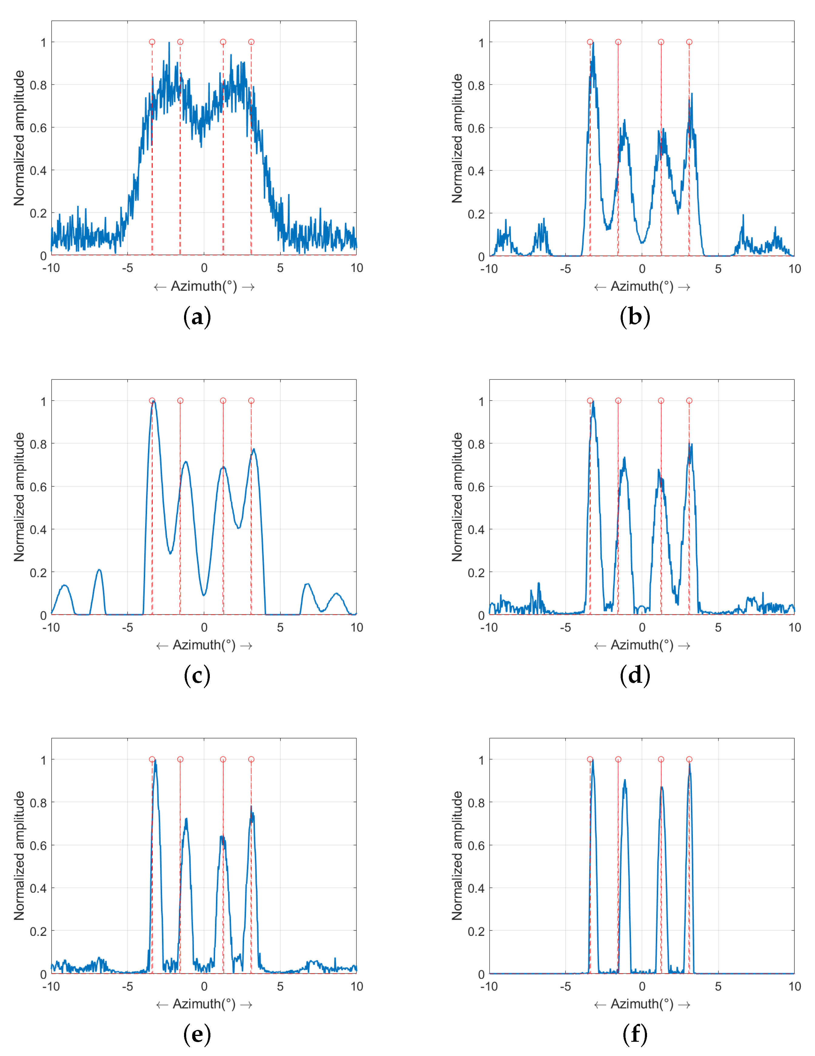
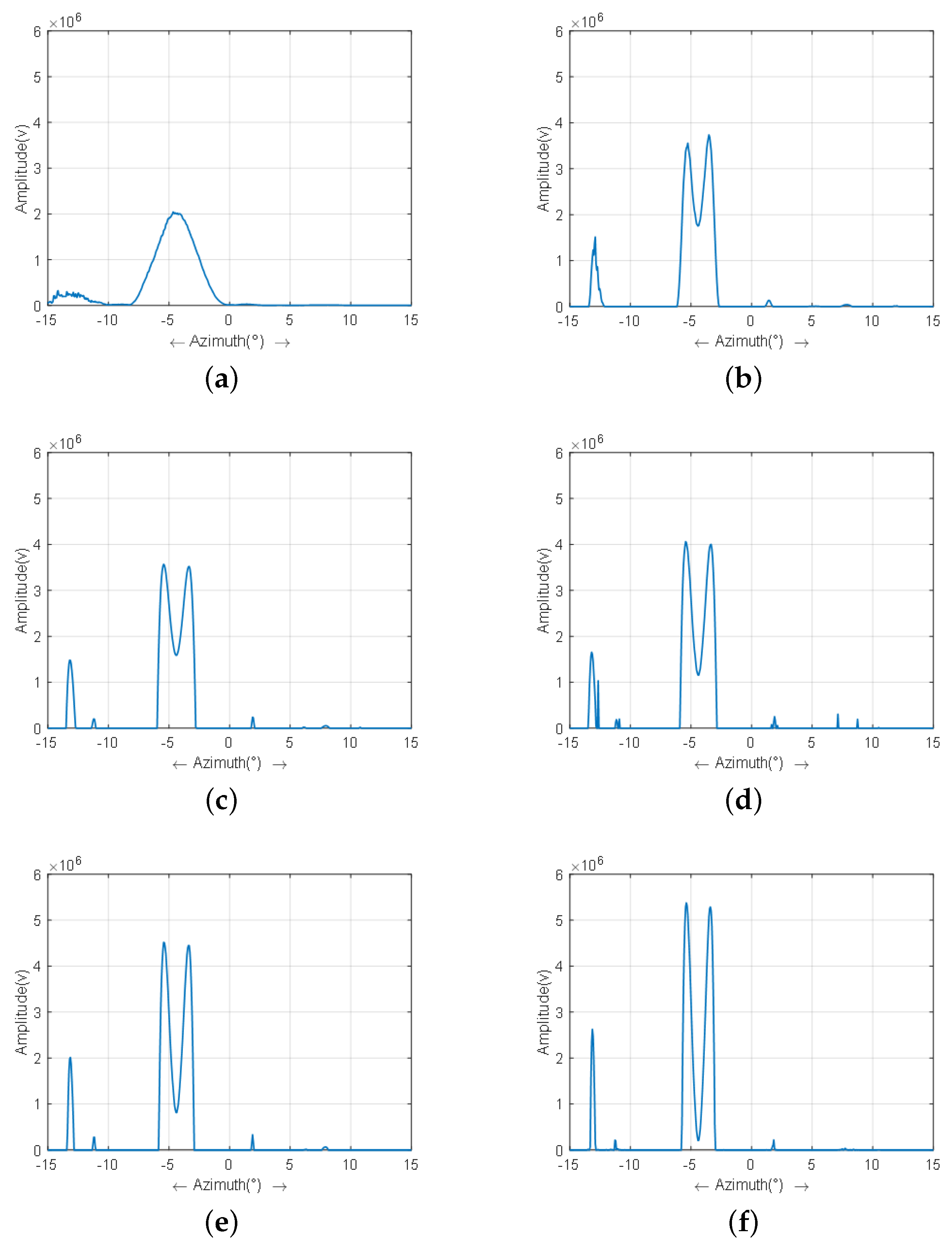
4.1. Experimental Results on Simulated Data

Figure 3a shows the simulated scene, which is composed of point targets settled in an X shape. The specific locations of those targets are shown in Figure 3a. The scattering coefficients are all set to 1 and do not change with time. The relevant experiment parameters are stated in

Table 1. Experiment parameters.

Parameters	Value
Velocity of the platform	100 m/s
Pulse repetition frequency	2000 Hz
Main-lobe beam width	$2^{\circ }$
Antenna scanning velocity	${60}^{\circ }/\mathrm{s}$
Antenna scanning area	${\pm 10}^{\circ }$
Near range	2.97 km

. We assume that there is no distortion in the antenna pattern over a sweep, which is a rational hypothesis for the low-speed platform. Figure 3b,c display the original echo and the echo after range compression and migration correction, separately. Figure 3d shows the enlarged version of the area where the target echo is located. It can be observed from Figure 3c,d that part of the echo energy of two X is overlapped, and the shape of X is difficult to identify.

Afterwards, the Gaussian white noise is superimposed onto the complex echo. The polluted data are displayed in Figure 4a, and the SNR equals 20 dB. Then, the echo in Figure 4a is processed by the proposed MAP-MRF method and four benchmarking methods, which are the classical Richardson–Lucy (RL) algorithm [28], the Tikhonov method [11], the L1-norm regularization method [12], and the sparse-TV method [15], respectively. All of these methods adopt the discrepancy criterion to stop the iterations [29]. Their outcomes are presented in Figure 4b–f, respectively.

The result of the RL algorithm is displayed in Figure 4b, from which it can be observed that the shapes of two X are basically restored. However, the edges of X are still fuzzy. Figure 4c displays the outcome of the Tikhonov method, in which the result is over-smoothed and the edges tend to be wide. The result of the L1-norm regularization method is displayed in Figure 4d. Due to the utilization of sparse prior information, the edges are much sharper. Nevertheless, some noise is mistreated as targets in the result. Hence, the result is presented as dispersed. Figure 4e displays the result of the sparse-TV method, which adds TV prior information to describe the continuity of the scene. Even though the outline is much clearer in Figure 4e, some unwanted energy still remains, especially near the edges. Figure 4f demonstrates the result of the proposed method. It is clear that the energy is better focused where the targets are located and that the shape of X is recovered much more clearly than by other benchmarking methods.

The profiles of the targets at 2987 m are illustrated in Figure 5, in which the dotted red line is where the targets are located. Figure 5a shows the profile of the echo, from which it can be seen that the echo of four targets are aliasing and the targets cannot be distinguished. Figure 5b,c show the profiles of the RL algorithm and Tikhonov method, respectively. It can be observed that the four targets have been partly recovered. However, the resolution needs to be strengthened further. Figure 5e is the profile of the L1-norm regularization method, in which the resolution has been improved compared with that in Figure 5b,c, but some unwanted false structures have emerged between the real targets. Figure 5e shows the profile of the sparse-TV method. Even the false structures have been suppressed to a certain extent, though some residual energy still exists. Figure 5f demonstrates the outcome of the MAP-MRF method. It is obvious that the four targets have been authentically restored, and the surroundings are fairly clear.

Next, the noise level of the echo is raised and the SNR is decreased to 10 dB. Then, the echo is processed by the five super-resolution imaging methods, respectively. Figure 6b displays the results of the RL algorithms, in which the results are severely distorted by the noise, and the structures of X can barely be distinguished. The result of the Tikhonov method is displayed in Figure 6c, and it can be observed that the noise has been smoothed, but so are the targets. Figure 6d demonstrates the results of the L1-norm regularization method. It can be seen that the edges are much clearer, but that the energy has been discretized, and the edge appears to be granular. The results of the sparse-TV method are displayed in Figure 6e. In comparison with Figure 6d, the energy of the edges is presented to be very continuous. However, the background contains some artifacts. Figure 6f demonstrates the outcome of MAP-MRF. It is clear that the edges are sharper, and the surroundings are much clearer, which indicates that the proposed method still has a strong performance in structure reconstruction in low-SNR conditions.

Figure 7 illustrates the profiles of the results in Figure 6. Figure 7b–e show the results of the benchmarking methods, from which it can be observed that there are some artifacts arising due to the high level of noise. The better the targets recovered are, the more obvious the artifacts are. However, it can be viewed from Figure 7f that not only are the restored targets the closest to the authentic targets, but that the artifacts are well suppressed.

In addition, the relative error (ReErr) and structure similarity (SSIM) are used to evaluate the performance of the acquired outcomes quantitatively. The specific definitions of ReErr and SSIM can be found in Reference [30], in which ReErr is used to evaluate the energy discrepancy between the result and the authentic targets, while SSIM is used to evaluate the structure similarity between the two compared subjects.

Figure 8 demonstrates the obtained ReErr and SSIM curves of the proposed method and benchmarking methods versus SNR. As we all know, noise will exert a huge influence on the performance of super-resolution algorithms. Thus, as viewed from Figure 8a, the ReErrs of all the super-resolution methods decline along with the increase in SNR. Among all the acquired curves, the one for the MAP-MRF method is at the bottom-most, which suggests that the outcome of MAP-MRF is the closest to the authentic solution. Notably, when SNR equals 0 dB, the ReErr of the MAP-MRF method is much smaller than that of the contrasted methods, which demonstrates the more favorable behavior of the MAP-MRF in low-SNR situations. In Figure 8b, the SSIMs of the MAP-MRF method are always on top, which indicates that the structure of MAP-MRF is the closest to that of the authentic scene, as well as verifying the comparison results of ReErr. In summary, the MAP-MRF method has more prominent advantages when the noise level is high and can recover the original scene more accurately than other similar methods.

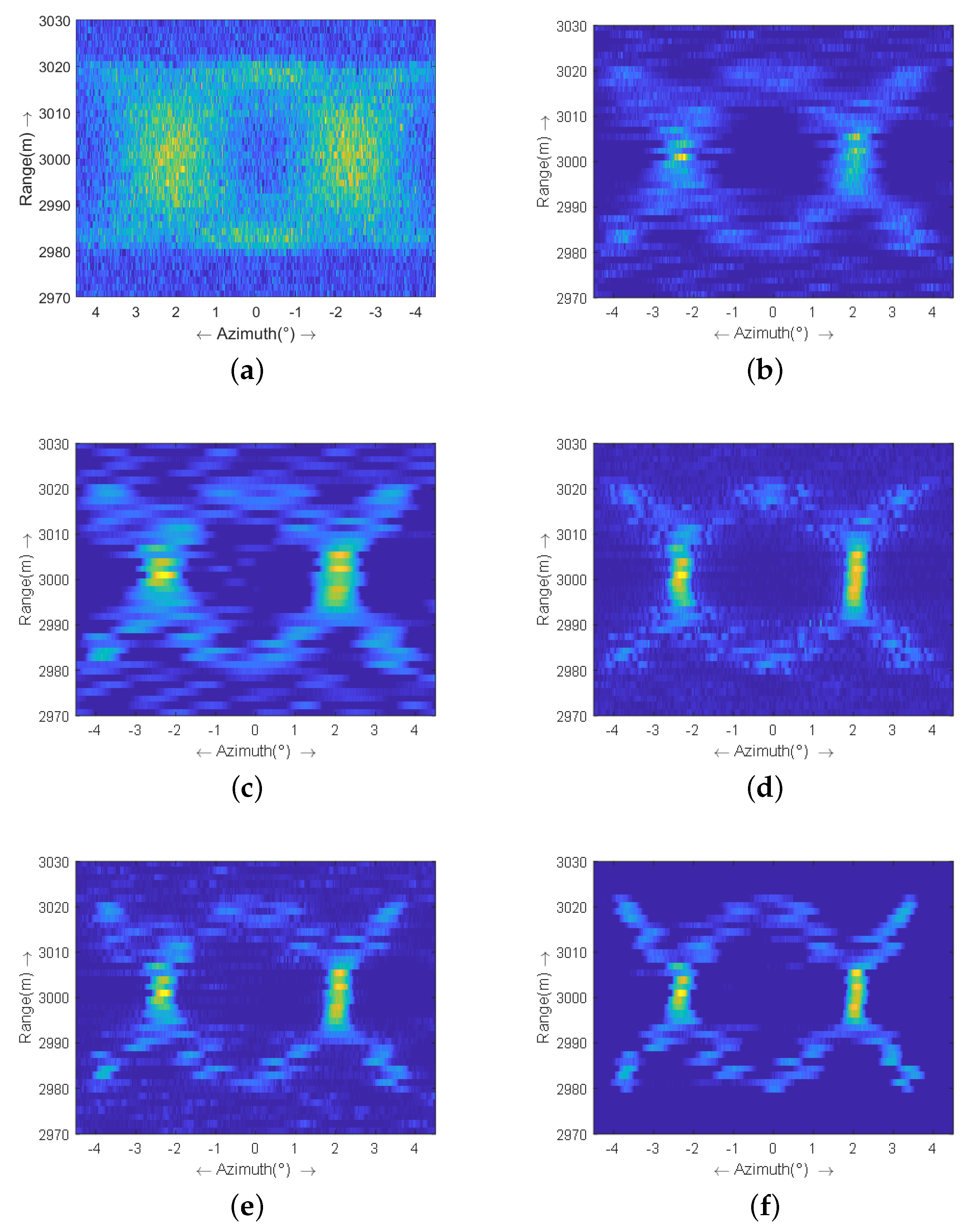
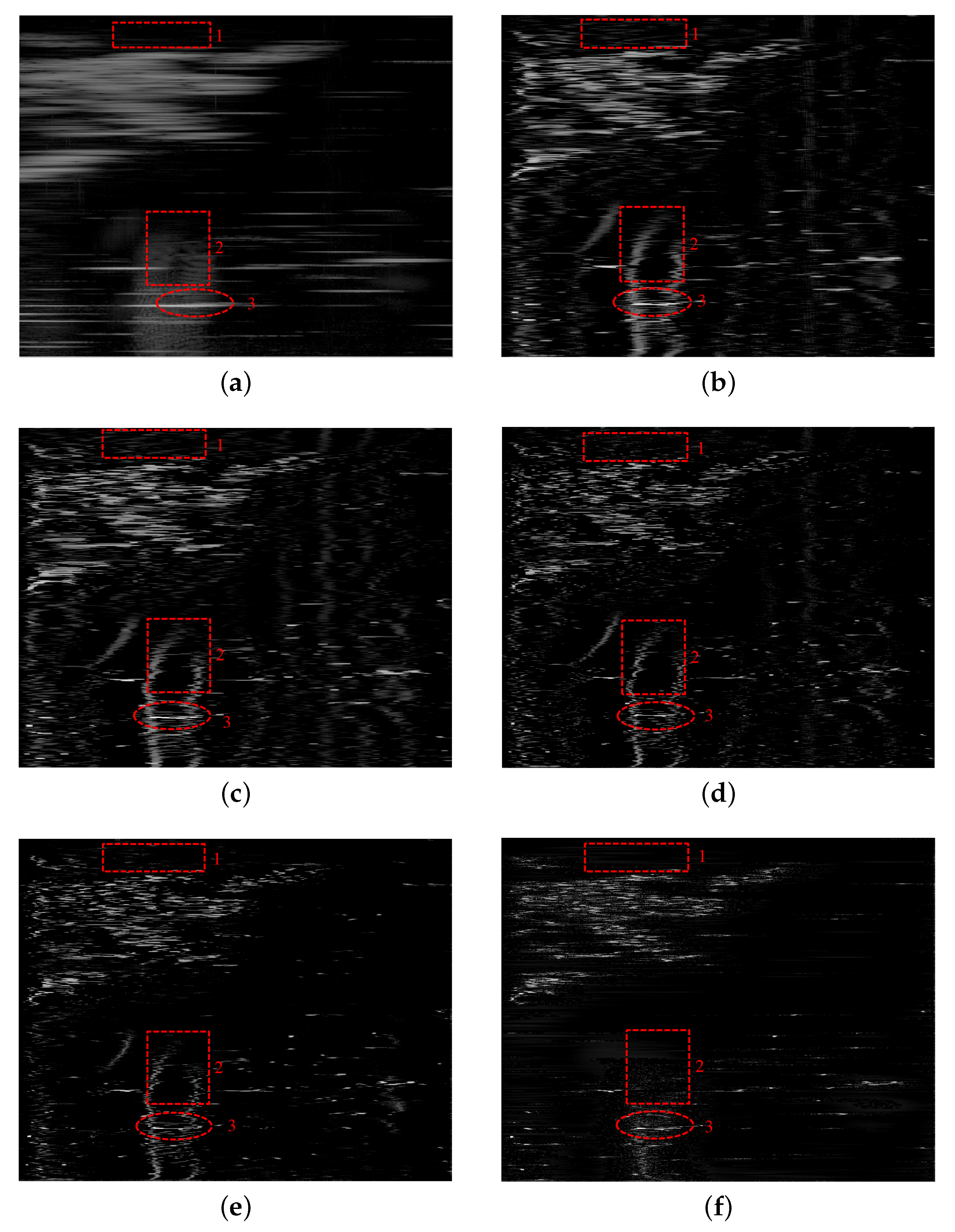
4.2. Experimental Results on Real Radar Data

The real data are processed in this subsection to demonstrate the validity and superiority of the MAP-MRF method. Figure 9 illustrates an optical picture of a scene in which an island is located in the upper side of the scene, and multiple ships are cruising across the sea surface. It is worth noting that the picture was captured from Google Maps, and the ships are only used for a schematic. A scanning radar whose antenna beam width is $2.5^{\circ }$ is settled on another island and sweeps the imaging scene.

Figure 10a shows the real beam image of the scene, from which it can be observed that the contour of the island is blurred, and the azimuth echoes of all ships are broadened. Since the incidence angle of the electromagnetic waves is relatively small, and the sea surface identified by red block 1 is partly shielded by the ridges of the island, there is almost no scattering energy in this region. The area identified by red block 2 is the range side lobe of two meeting ships’ echo compressed by the matched filtering. The area marked by red ellipse 3 is the two meeting ships. It can be observed that the echo energy in the azimuth is broadened and superimposed, which results in the two ships being indistinguishable. Then, the benchmarking methods and the proposed MAP-MRF method are both used on the echo. Figure 10b–e show the results of contrasted methods. It can be seen that the resolution has been partly enhanced and the contour of the island is sharpened. However, in the sea surface identified by red block 1, some artifacts are aroused after the super-resolution process. Furthermore, the side lobe marked by red block 2 is transformed into long tails in the range direction after the process. Figure 10f illustrates the result of the proposed method, in which the outline of the island is fairly clear, and there are almost no false targets in the area of red block 1. The side lobe in red block 2 is also suppressed due to the use of structural information.

Figure 11 presents the profiles of the ships marked by red ellipse 3 of all the outcomes. From Figure 11b–d, it can be seen that the sparse Bayesian method performs best in distinguishing the two ships. However, some spurious structures appear. Figure 11e shows the results of the sparse-TV method, in which the spurious structure has been eliminated. Figure 11f demonstrates the result of MAP-MRF, in which not only are the ships well separated, but there is also no increase in the noise. In summary, the results of the real data experiment indicate that MAP-MRF can achieve a high super-resolution ratio with no noise amplification and recover the contour of the scenario better than the contrasted methods can.

5. Discussion

In the imaging task, the 2-D spatial structure information plays an important role in image processing. However, even though a certain number of prior information has been discovered in state-of-the-art literature, e.g., sparse prior, square-norm prior, TV prior, or the combination of those priors, all those methods are conducted on one profile of the echo each time; thus, only one-dimensional (1-D) prior information is utilized. The MRF theory provides a powerful approach to exploit the 2-D structural character of images, which is of great significance for improving the resolution and recovering the structure information. Therefore, coupled with accurate noise modeling, the MAP-MRF can perform pretty well in noise resistance and structure recovery. Besides, the Huber function is chosen as the specific form for MRF, of which diverse penalties can effectively protect the edge information. For the visual and quantitative results obtained in Section 4, the proposed MAP-MRF method can retrieve the structure and contour of the scene more accurately compared with the benchmarking methods, especially in the low-SNR condition.

It should be noted that some assumptions are made in this paper. First, the convolution kernel is formulated as a cyclic-convolution matrix to decrease the computational complexity. Even though some end-part of the result may be inaccurate, this formulation can greatly reduce the calculation through FFT operation. As to the minute inaccurate part, it can be discarded after super-resolution processing. The second is that the scattering coefficients are set to be constant in the model. Even though this may differ from the real-life situation, this assumption is adopted for the modeling simplicity and will not affect the efficiency of the method itself. Moreover, The real data has validate its effectiveness.

Furthermore, some improvement work can continue to be completed. For instance, the high-order neighborhood systems are encouraged to be further investigated in future work. In addition, energy function should also be optimized according to diverse imaging scene.

6. Conclusions

Super-resolution technology is inherently an ill-conditioned issue, and the results are susceptible to noise. Prior information plays a crucial role in the process of resolving the issue. In this paper, an MAP-MRF model is exploited for RASR super-resolution imaging. Through making use of the MRF model, the structural prior information in the scene can be deeply exploited. Firstly, the MAP framework is utilized to construct the objective function for RASR super-resolution imaging. Then, the imaging scene is modeled by the HMRF and the spatial structural information is utilized to reconstruct the scene. Finally, by solving the objective function with an accelerated iterative solution strategy, the optimal super-resolution result of the targets can be obtained. Contrasted with traditional super-resolution methods, the MAP-MRF method can retrieve the shape of the scene much more clearly when improving the angular resolution.

References

1. Peng, X.; Wang, Y.; Hong, W.; Tan, W.; Wu, Y. Autonomous navigation airborne forward-looking SAR high precision imaging with combination of pseudo-polar formatting and overlapped sub-aperture algorithm. Remote Sens. 2013, 5, 6063–6078. [Google Scholar] [CrossRef] [Green Version]
2. Xia, J.; Lu, X.; Chen, W. Multi-channel deconvolution for forward-looking phase array radar imaging. Remote Sens. 2017, 9, 703. [Google Scholar] [CrossRef] [Green Version]
3. Curlander, J.C.; McDonough, R.N. Synthetic Aperture Radar: Systems and Signal Processing; Wiley: New York, NY, USA, 1991; Volume 199. [Google Scholar]
4. Tang, S.; Guo, P.; Zhang, L.; Lin, C. Modeling and precise processing for spaceborne transmitter/missile-borne receiver SAR signals. Remote Sens. 2019, 11, 346. [Google Scholar] [CrossRef] [Green Version]
5. Wu, D.; Zhu, D.Y.; Zhu, Z.D. Research on nomopulse forward-looking imaging algorithm for airborne radar. J. Image Graph. 2010, 15, 462–469. [Google Scholar]
6. Chen, H.; Lu, Y.; Mu, H.; Yi, X.; Liu, J.; Wang, Z.; Li, M. Knowledge-aided mono-pulse forward-looking imaging for airborne radar by exploiting the antenna pattern information. Electron. Lett. 2017, 53, 566–568. [Google Scholar] [CrossRef]
7. Zhang, Y.; Zhang, Y.; Huang, Y.; Li, W.; Yang, J. Angular superresolution for scanning radar with improved regularized itera-tive adaptive approach. IEEE Geosci. Remote Sens. Lett. 2016, 13, 846–850. [Google Scholar] [CrossRef]
8. Zhang, Y.; Zhang, Y.; Li, W.; Huang, Y.; Yang, J. Super-resolution surface mapping for scanning radar: Inverse filtering based on the fast iterative adaptive approach. IEEE Geosci. Remote Sens. Lett. 2017, 56, 127–144. [Google Scholar] [CrossRef]
9. Zhang, Q.; Zhang, Y.; Zhang, Y.; Huang, Y.; Yang, J. A Sparse Denoising-Based Super-Resolution Method for Scanning Radar Imaging. Remote Sens. 2021, 13, 2768. [Google Scholar] [CrossRef]
10. Liu, P.Y.; Keenan, D.M.; Kok, P.; Padmanabhan, V.; O’Byrne, K.T.; Veldhuis, J.D. Sensitivity and specificity of pulse detection using a new deconvolution method. Am. J. -Physiol.-Endocrinol. Metab. 2009, 297, E538–E544. [Google Scholar] [CrossRef] [Green Version]
11. Egger, H.; Engl, H.W. Tikhonov regularization applied to the inverse problem of option pricing: Convergence analysis and rates. Inverse Probl. 2005, 21, 1027. [Google Scholar] [CrossRef] [Green Version]
12. Chen, H.M.; Li, M.; Wang, Z.; Lu, Y.; Zhang, P.; Wu, Y. Sparse super-resolution imaging for airborne single channel forward-looking radar in expanded beam space via lp regularisation. Electron. Lett. 2015, 15, 863–865. [Google Scholar] [CrossRef]
13. Tuo, X.; Zhang, Y.; Huang, Y.; Yang, J. Fast sparse-TSVD super-resolution method of real aperture radar forward-looking imaging. IEEE Geosci. Remote Sens. Lett. 2020, 59, 6609–6620. [Google Scholar] [CrossRef]
14. Zhang, Y.; Tuo, X.; Huang, Y.; Yang, J. A tv forward-looking super-resolution imaging method based on tsvd strategy for scanning radar. IEEE Geosci. Remote Sens. Lett. 2020, 58, 4517–4528. [Google Scholar] [CrossRef]
15. Zhang, Q.; Zhang, Y.; Huang, Y.; Zhang, Y.; Pei, J.; Yi, Q.; Yang, J. TV-sparse super-resolution method for radar for-ward-looking imaging. IEEE Geosci. Remote Sens. Lett. 2020, 58, 6534–6549. [Google Scholar] [CrossRef]
16. Tuo, X.; Zhang, Y.; Huang, Y.; Yang, J. Fast total variation method based on iterative reweighted norm for airborne scanning radar super-resolution imaging. Remote Sens. 2020, 12, 2877. [Google Scholar] [CrossRef]
17. Guan, J.; Yang, J.; Huang, Y.; Li, W. Maximum a posteriori based angular superresolution for scanning radar imaging. IEEE Trans. Aerosp. Electron. Syst. 2014, 50, 2389–2398. [Google Scholar] [CrossRef]
18. Zha, Y.; Huang, Y.; Sun, Z.; Wang, Y.; Yang, J. Bayesian deconvolution for angular super-resolution in forward-looking scan-ning radar. Sensors 2015, 15, 6924–6946. [Google Scholar] [CrossRef] [PubMed] [Green Version]
19. Tan, K.; Li, W.; Pei, J.; Huang, Y.; Yang, J. An I/Q-channel modeling maximum likelihood super-resolution imaging method for forward-looking scanning radar. IEEE Geosci. Remote Sens. Lett. 2018, 15, 863–867. [Google Scholar] [CrossRef]
20. Tan, K.; Li, W.; Zhang, Q.; Huang, Y.; Wu, J.; Yang, J. Penalized maximum likelihood angular super-resolution method for scanning radar forward-looking imaging. Sensors 2018, 18, 912. [Google Scholar] [CrossRef] [Green Version]
21. Li, W.; Yang, J.; Huang, Y. Keystone transform-based space-variant range migration correction for airborne forward-looking scanning radar. Electron. Lett. 2012, 48, 121–122. [Google Scholar] [CrossRef]
22. Rajagopalan, A.N.; Chaudhuri, S. An MRF model-based approach to simultaneous recovery of depth and restoration from defocused images. IEEE Trans. Pattern Anal. Mach. Intell. 1999, 21, 577–589. [Google Scholar] [CrossRef] [Green Version]
23. Gleich, D. Markov random field models for non-quadratic regularization of complex SAR images. IEEE J. Sel. Top. Appl. Earth Obs. Remote. Sens. 2012, 5, 952–961. [Google Scholar] [CrossRef]
24. Panić, M.; Aelterman, J.; Crnojević, V.; Pižurica, A. Sparse recovery in magnetic resonance imaging with a Markov random field prior. IEEE Trans. Med. Imag. 2017, 36, 2104–2115. [Google Scholar] [CrossRef]
25. Soccorsi, M.; Gleich, D.; Datcu, M. Huber–Markov model for complex SAR image restoration. IEEE Geosci. Remote Sens. Lett. 2009, 7, 63–67. [Google Scholar] [CrossRef]
26. Hansen, P.C.; O’Leary, D.P. The use of the L-curve in the regularization of discrete ill-posed problems. SIAM J. Sci. Comput. 1993, 14, 1487–1503. [Google Scholar] [CrossRef]
27. Tan, K.; Li, W.; Huang, Y.; Zhang, Q.; Zhang, Y.; Wu, J.; Yang, J. Vector extrapolation accelerated iterative shrink-age/thresholding regularization method for forward-looking scanning radar super-resolution imaging. J. Appl. Remote Sens. 2018, 12, 045016. [Google Scholar]
28. Su, L.; Shao, X.; Wang, L.; Wang, H.; Huang, Y. Richardson-lucy deblurring for the star scene under a thinning motion path. In Satellite Data Compression, Communications, and Processing XI; International Society for Optics and Photonics: Bellingham, DC, USA, 2015; Volume 9501, p. 95010L. [Google Scholar]
29. Li, G.; Piccolomini, E.L.; Tomba, I. A stopping criterion for iterative regularization methods. Appl. Numer. Math. 2016, 106, 53–68. [Google Scholar]
30. Xu, G.; Sheng, J.; Zhang, L.; Xing, M. Performance improvement in multi-ship imaging for ScanSAR based on sparse rep-resentation. Sci. China Inf. Sci. 2012, 55, 1860–1875. [Google Scholar] [CrossRef]
Figure 1. The imaging sketch of RASR.
Remotesensing 13 04115 g001
Figure 2. (a) The fifth-order neighborhood; (b) cliques for the first-order neighborhood; (c) cliques for the second-order neighborhood.
Remotesensing 13 04115 g002
Figure 3. (a) Simulation scene; (b) original echo; (c) echo after range compression and migration correction; (d) enlarged targets.
Remotesensing 13 04115 g003
Figure 4. Comparison of the super-resolution results in the case of S N R = 20 dB: (a) echo; (b) RL algorithm; (c) Tikhonov method; (d) L1-norm regularization method; (e) sparse-TV method; and (f) proposed MAP-MRF method.
Remotesensing 13 04115 g004
Figure 5. The profile of super-resolution outcomes in the case of S N R = 20 dB: (a) echo; (b) RL algorithm; (c) Tikhonov method; (d) L1-norm regularization method; (e) sparse-TV method; and (f) proposed MAP-MRF method.
Remotesensing 13 04115 g005
Figure 6. Super-resolution results comparison in the case of S N R = 10 dB: (a) echo; (b) RL algorithm; (c) Tikhonov method; (d) L1-norm regularization method; (e) sparse-TV method; and (f) proposed MAP-MRF method.
Remotesensing 13 04115 g006
Figure 7. The profile of super-resolution results in the case of S N R = 10 dB: (a) echo (b) RL algorithm; (c) Tikhonov method; (d) L1-norm regularization method; (e) sparse-TV method; and (f) proposed MAP-MRF method.
Remotesensing 13 04115 g007
Figure 8. Quantitative curves for different super-resolution methods: (a) ReErr; (b) SSIM.
Remotesensing 13 04115 g008
Figure 9. The imaging sketch of RASR.
Remotesensing 13 04115 g009
Figure 10. Real data experiment: (a) echo; (b) RL algorithm; (c) Tikhonov method; (d) L1-norm regularization method; (e) sparse-TV method; and (f) proposed MAP-MRF method.
Remotesensing 13 04115 g010
Figure 11. Profiles of the super-resolution results of real data: (a) echo; (b) RL method; (c) Tikhonov method; (d) L1-norm regularization method; (e) sparse-TV method; and (f) proposed MAP-MRF method.
Remotesensing 13 04115 g011