
A High-Resolution, Random Forest Approach to Mapping Depth-to-Bedrock across Shallow Overburden and Post-Glacial Terrain

Abstract
:1. Introduction
2. Methods
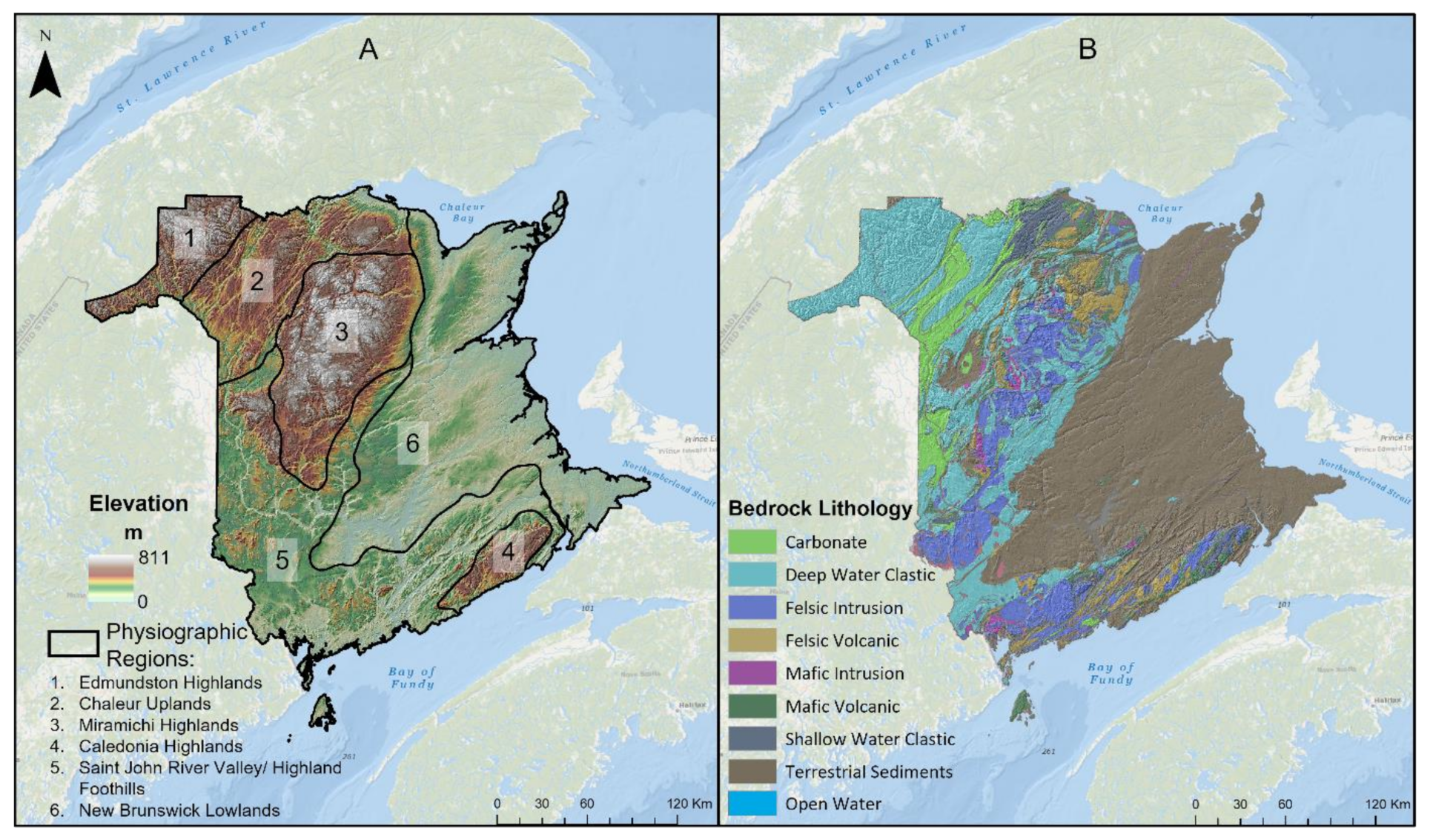
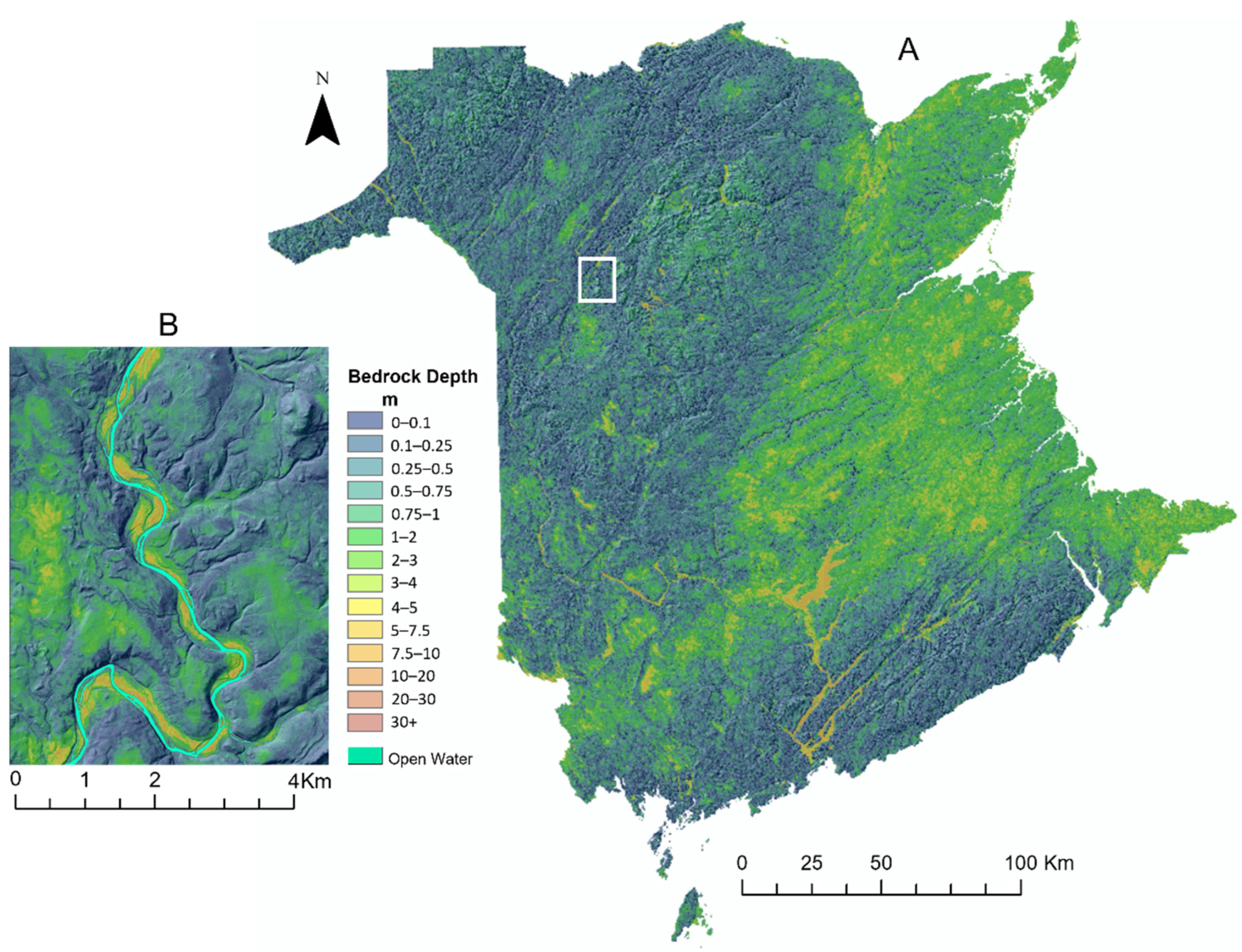
2.1. Study Region
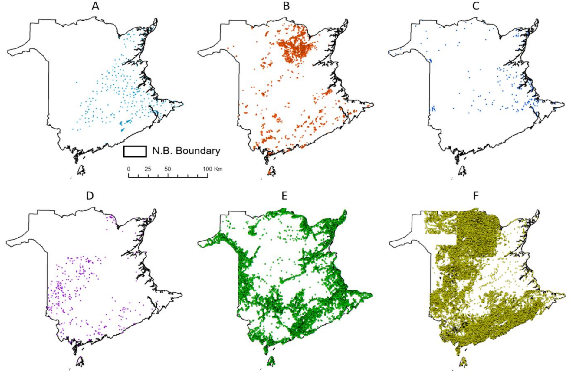
2.2. Regolith and DTB Data Sources
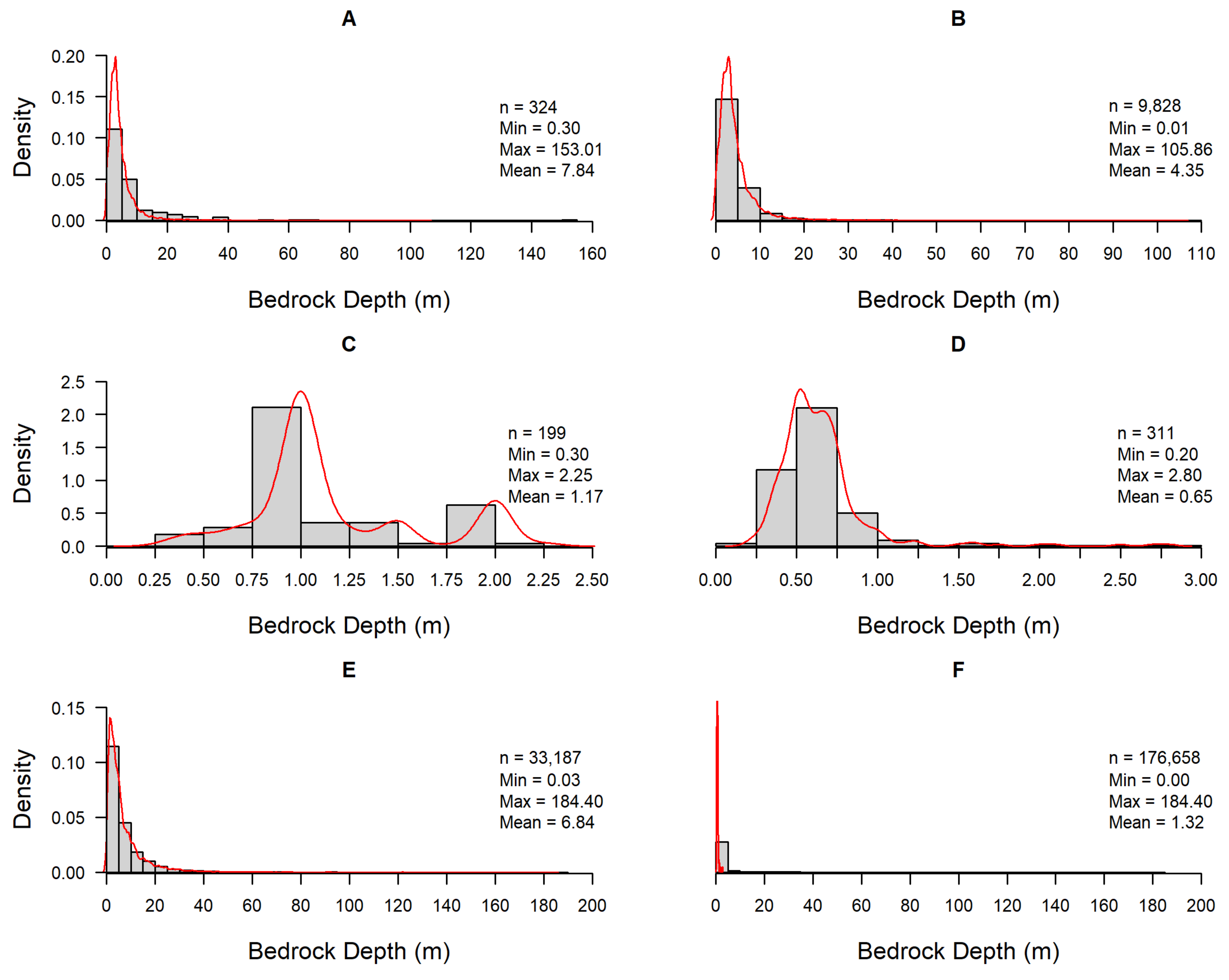
- Boreholes: A borehole database was accessed from NB Department of Energy and Resource Development (NBERD) via a national topographic system (NTS) index [32]. These data represent the results of petroleum, potash, and coal production/exploration (n = 332).
- Drillholes: This database is an amalgamation of drill holes collected as part of diamond drilling mineral exploration within the province. DTB was recorded in exploration reports. These data were accessed from Service New Brunswick’s GeoNB data catalogue [21] (n = 9,828).
- Pedons: Soil samples collected as part of multiple research projects, including the development of county-based soil surveys by the Canadian Soil Information Service [33] and a permanent sample plot database from NBERD [34]. From the databases, samples were queried and selected for those with DTB recorded (n = 199).
- Site Cards: A set of till geochemistry site cards exist that represent till geochemistry surveys conducted throughout NB. Site cards were retrieved from the geoscience publication search query [35] and limiting search results to open file reports. These data were amalgamated and only samples with DTB measurements were selected for analyses (n = 324).
- Well Logs: This dataset represents the recorded data for all new and deepened drinking water wells in NB since 1994, amalgamated by the New Brunswick Department of Environment and Local Government (NBELG). The depth at which bedrock was contacted was also recorded in the dataset. This information was retrieved from GeoNB data catalogue [21] (n = 33,187).
- Rock Outcrops: the rock outcrops represent the results of on-ground transects conducted throughout the province to locate areas in which bedrock was exposed at the surface (NBERD) (n = 126,849).
2.3. Data Quality Assessment
2.4. Modelling Framework
2.5. Model Parameters
2.5.1. Geological Data
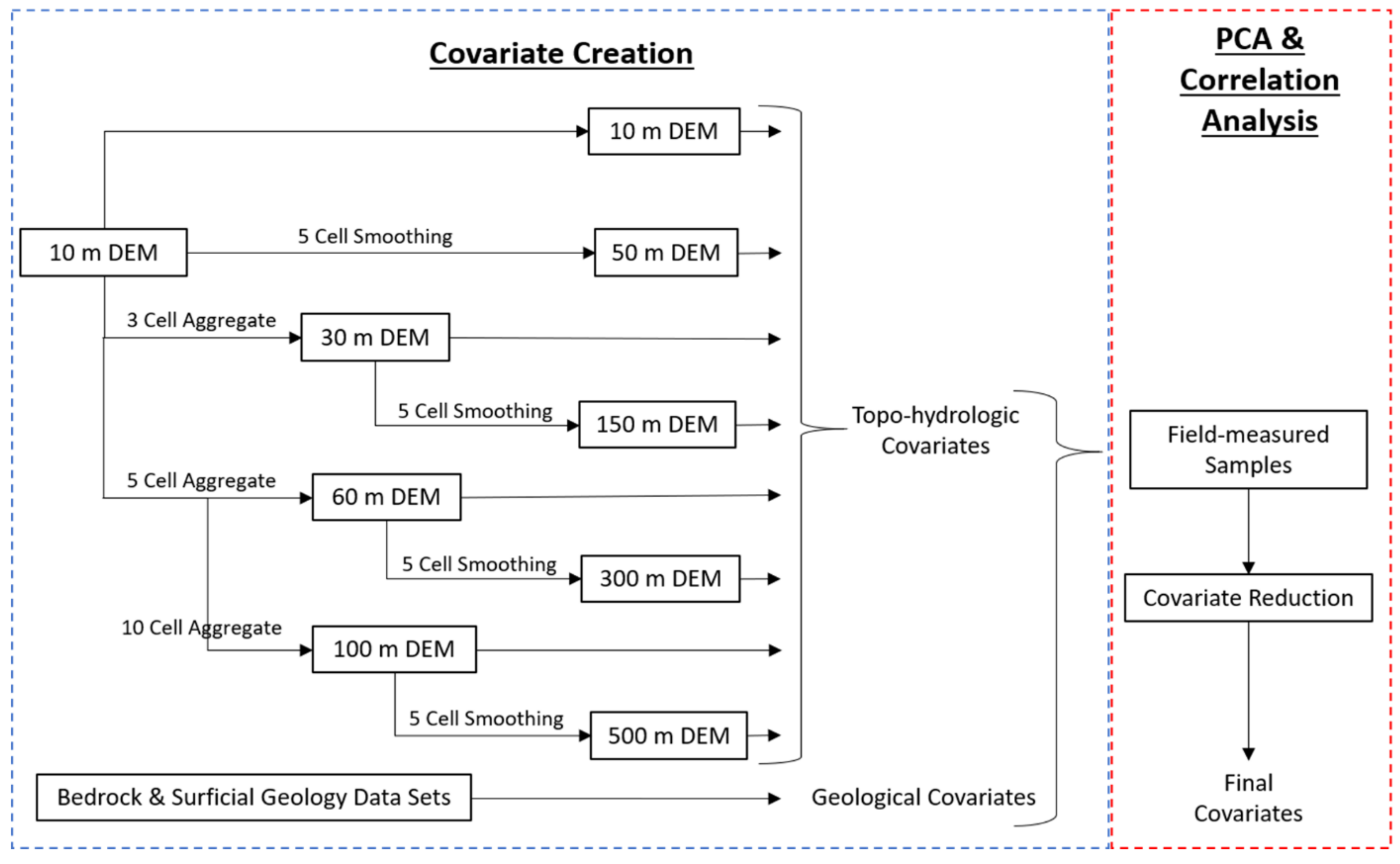
2.5.2. Topo-Hydrological Data
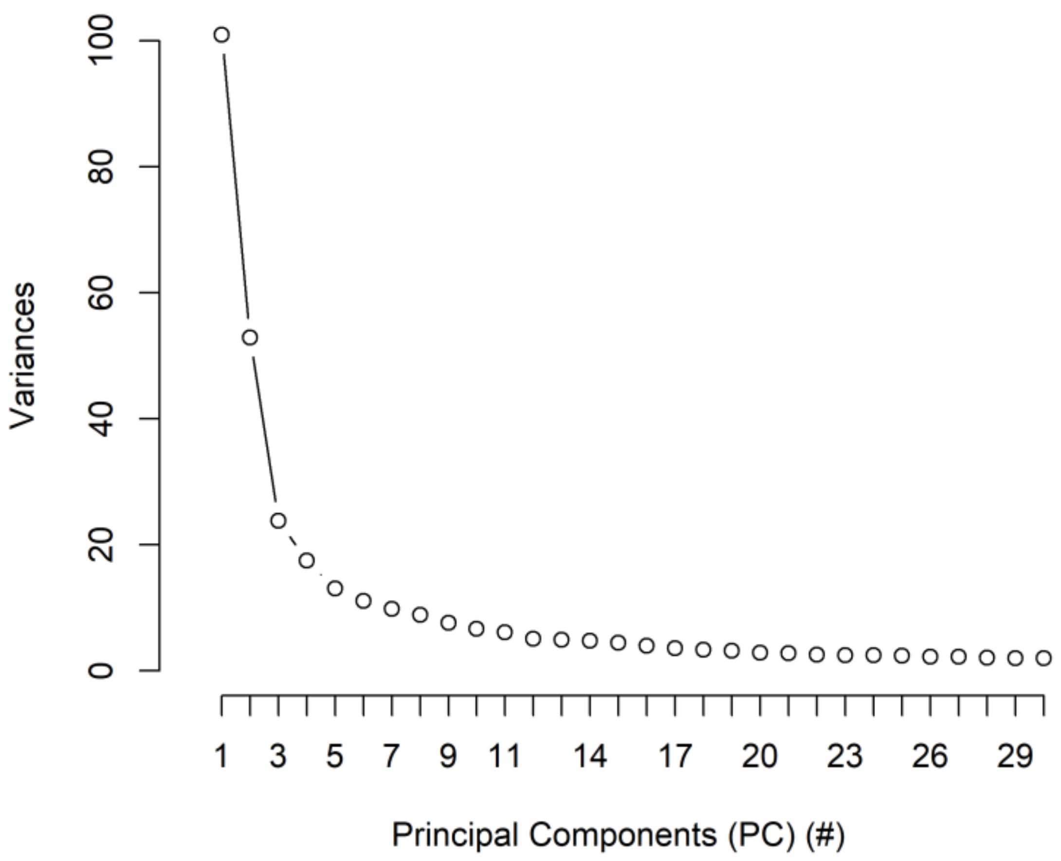
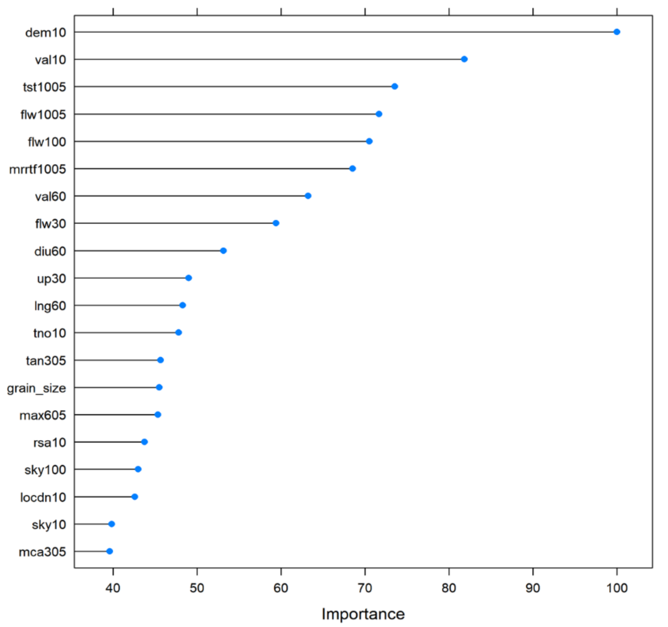
2.5.3. Covariate Reduction
2.6. Statistical Modeling
3. Results
3.1. Covariate Reduction
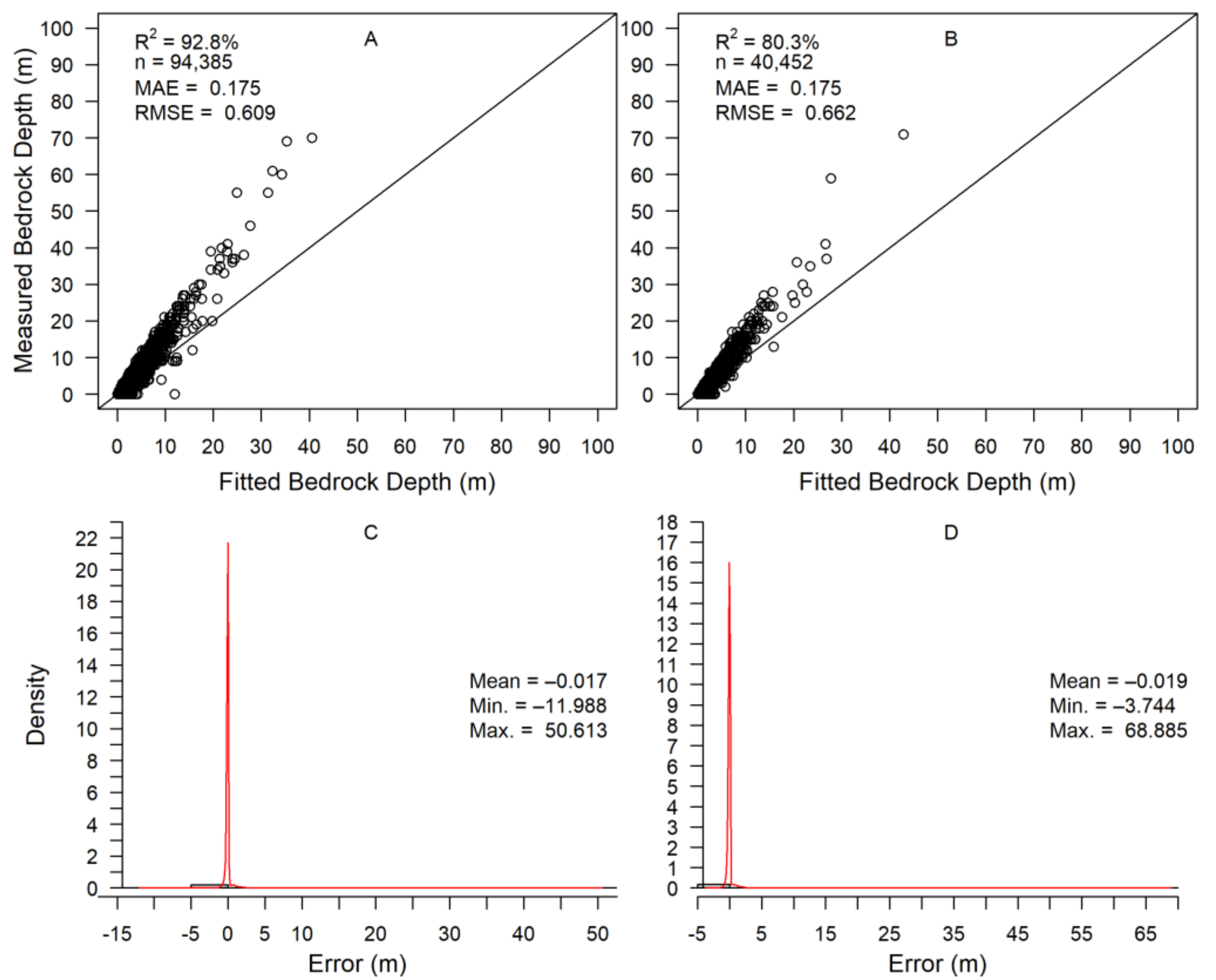
3.2. Model Results
4. Discussion
4.1. Depth-to-Bedrock Model
4.2. Limitations & Uncertainties
5. Conclusions
Author Contributions
Funding
Institutional Review Board Statement
Informed Consent Statement
Data Availability Statement
Acknowledgments
Conflicts of Interest
Appendix A

| Covariate | Abbreviation | Definition | Reference | Software Used |
|---|---|---|---|---|
| Aggregate | Agg1_0 | Binary representing if a cell falls within a delineated aggregate deposit or not. | This study | ArcGIS |
| Distance to Aggregate | Agg_Dist | Euclidean (horizontal) distance to aggregate deposit | This Study | ArcGIS |
| Aspect | Asp | Cardinal direction of slope (measured in degrees) | [38,39] | SAGA GIS |
| Bedrock Age | Bed_age | Average age of bedrock geology types across New Brunswick | This Study | ArcGIS |
| Catchment Area | Ca | Upslope area contributing discharge into any given cell, calculated from flow accumulation | [40,41] | ArcGIS |
| Catchment Slope | Cs | Slope of catchment, derived as intermediate with SAGA Wetness Index | [42,43] | SAGA GIS |
| Convergence Index (gradient) | Cvgr | Determines the convergence or divergence based on neighboring cells (calculated using gradient) | [44] | SAGA GIS |
| Convergence Index (aspect) | Cvas | Determines the convergence or divergence based on neighboring cells (calculated using aspect) | [44] | SAGA GIS |
| Cross-sectional Curvature | Crs | Like planar curvature | [38] | SAGA GIS |
| Distance to Waterbody | Wb_Dist | Euclidean (horizontal) distance to delineated waterbody | This study | ArcGIS |
| Distance to Wetland | Wetland | Euclidean (horizontal) distance to delineated wetland | This study | |
| Diurnal Anistropic Heating | Diu | Influence of topography on diurnal heat balance | [45] | SAGA GIS |
| Curvature Classification | Cur | Representation of surface curvature/9 geometric forms of hillslopes | [46,47] | SAGA GIS |
| Downslope Curvature | Dwn | Like profile curvature | [40] | SAGA GIS |
| Downward Distance Gradient | Dwd | Measures impact of local slope on hydraulic gradient | [49] | SAGA GIS |
| Digital Elevation Model | Dem | Representation of elevation change across landscape, height above sea level | [50,51] | ArcGIS |
| Filled DEM | Fi | Depression-filled version of the DEM | [52] | SAGA GIS |
| Flowline Curvature | Flw | Like profile curvature | [40] | SAGA GIS |
| General Curvature | Gen | Combination of planar and profile curvature | [39] | SAGA GIS |
| Dominant Geology Type | Geo_class | Gridded representation of changing geological types (sedimentary, igneous, metamorphic) of parent material | This study | ArcGIS |
| Dominant Grain Size | Grain_class | Gridded representation of changing mineral sizes from very fine to coarse based on lithology of parent material | This study | ArcGIS |
| Horizontal Distance to Stream | St_hdist | Euclidean distance to nearest stream | This study | ArcGIS |
| Landform | Land_Class | Gridded representation of parent material (surficial geology) mode of deposition | This study | ArcGIS |
| Latitude | Lat | Gridded representation of changing latitude from north to south (decimal degree format) | This study | ArcGIS |
| Local Curvature | Loc | Calculates the total gradient to neighboring cells | [40] | SAGA GIS |
| Local Downslope Curvature | Locdn | Same as local curvature but only looks at downslope cells | [40] | SAGA GIS |
| Local Upslope Curvature | Locup | Same as local curvature but only looks at upslope contributing cells | [40] | SAGA GIS |
| Longitude | Long | Gridded representation of changing longitude from west to east (decimal degree format) | This study | ArcGIS |
| Longitudinal Curvature | Lng | Like profile curvature | [38] | SAGA GIS |
| Lithology | Lith_class | Gridded representation of parent material (surficial geology lithology) | This study | ArcGIS |
| Maximum Curvature | Max | Calculates the maximum slope of the slope on a defined search radius (secondary derivative) | [38,53,54,55] | SAGA GIS |
| Mineral Hardness | Hardness | Gridded representation of the hardness of lithologic types based on Moh’s hardness scale | This study | ArcGIS |
| Minimum Curvature | Min | Calculates the minimum slope of the slope on a defined search radius (secondary derivative) | [38,53,54,55] | SAGA GIS |
| Modified Catchment Area | Mca | Adjustment to catchment area calculation to correct for flow in low-lying flat areas. | [42,43] | SAGA GIS |
| Modified Specific Catchment Area | Msca | Modified version of Specific Catchment Area | [40] | SAGA GIS |
| Multi-resolution Index of Valley Bottom Flatness | Mrvbf | Delineation of valley bottom flatness from surrounding hillslopes | [56] | SAGA GIS |
| Multi-resolution Index of Ridge Top Flatness | Mrrtf | Delineation of ridgetops flatness from surrounding hillslopes, intermediate of MRVBF | [56] | SAGA GIS |
| Outcrop Distance | Out_Dist | Euclidean (horizontal) distance to rock outcrops | This study | ArcGIS |
| Planar Curvature | Pln | Curvature perpendicular to slope | [38] | SAGA GIS |
| Profile Curvature | Prf | Curvature parallel to slope | [38] | SAGA GIS |
| Real Surface Area | Rsa | Calculation of ‘real’ cell area | [57] | SAGA GIS |
| Dominant Rock Type | Rock_class | Gridded representation of changing rock types based on lithology of parent material | This study | ArcGIS |
| SAGA Wetness Index | Swi | Computes a modified topographic wetness index | [42,43] | SAGA GIS |
| Sky View Factor | Sky | Amount of sky hemisphere visible from the ground | [58,59,60] | SAGA GIS |
| Slope (%) | Slp | Rate of elevation change between adjacent cells (as %) | [38,39] | SAGA GIS |
| Slope Length | Sl | Determine the length of slope | [61] | SAGA GIS |
| Slope Length and Steepness | Ls | Calculates slope length factor, typically used in Revised Universal Soil Loss Equation (RUSLE) | [43,62,63] | SAGA GIS |
| Specific Catchment Area | Sca | Catchment area divided by cell width | [40] | SAGA GIS |
| Specific Catchment Slope | Scs | Catchment area divided by cell width | [42,43] | SAGA GIS |
| Tangential Curvature | Tan | Determines areas of convex and concave flows, calculated from planar and profile curvature | [39] | SAGA GIS |
| Terrain Ruggedness Index | Tri | Total change in elevation within a defined radius of any given cell | [64] | SAGA GIS |
| Terrain Surface Convexity | Tscv | Determines percentage of upward and convex cells within a defined radius | [65] | SAGA GIS |
| Terrain Surface Concavity | Tscc | Determines percentage of upward and concave cells within a defined radius, same algorithm as terrain surface convexity | [65] | SAGA GIS |
| Terrain Surface Texture | Tst | Determines the variability in frequency and intensity of pits and peaks within a defined radius | [65] | SAGA GIS |
| Terrain View Factor | Trn | Output covariate from Sky View Factor | [58,59,60] | SAGA GIS |
| Multi-scale Topographic Position Index | Tpi | Position on hillslope in relation to adjacent cells | [39,66] | SAGA GIS |
| 27Topographic Positive Openness | Tpo | Represents landscape exposure to atmosphere (positive) | [67] | SAGA GIS |
| Topographic Negative Openness | Tno | Represents landscape exposure to atmosphere (negative) | [67,68] | SAGA GIS |
| Total Curvature | Tot | Curvature of the surface | [39] | SAGA GIS |
| Upslope Curvature | Up | Average local curvature of upslope contributing area for any given cell | [40] | SAGA GIS |
| Valley Depth | Val | Like inverse of vertical distance to channel network | [69] | SAGA GIS |
| Vector Ruggedness Measure | Vrm | Quantifies landscape ruggedness via slope and aspect | [70] | SAGA GIS |
| Vertical Distance to Stream | St_vdist | Vertical distance from nearest stream based on increasing elevation | [71,72] | ArcGIS |
| View Distance | View | Average distance to horizon, output from Sky View Factor | [58,59,60] | SAGA GIS |
| Visible Sky | Vis | The percentage of unobstructed hemisphere, output from Sky View factor | [58,59,60] | SAGA GIS |
References
- Weil, R.R.; Brady, N.C. The Nature and Properties of Soils, 15th ed.; Fox, D., Gilfillan, A., Dimmick, L., Eds.; Pearson Education: Upper Saddle River, NJ, USA, 2017; ISBN 9780133254488. [Google Scholar]
- Yan, F.; Shangguan, W.; Zhang, J.; Hu, B. Depth-to-bedrock map of China at a spatial resolution of 100 meters. Science 2020, 7, 1–13. [Google Scholar]
- Gomes, G.J.C.; Vrugt, J.A.; Vargas, E.A., Jr. Toward improved prediction of the bedrock depth underneath hillslopes: Bayesian inference of the bottom-up control hypothesis using high-resolution topographic data. Water Resour. Res. 2016, 52, 3085–3112. [Google Scholar] [CrossRef] [Green Version]
- Devkota, S.; Shakya, N.M.; Sudmeier, K.; McAdoo, B.G.; Jaboyedoff, M. Predicting soil depth to bedrock in an anthropogenic landscape: A case study of Phewa Watershed in Panchase region of Central-Western Hills, Nepal. J. Nepal Geol. Soc. 2018, 55, 173–182. [Google Scholar] [CrossRef]
- Shangguan, W.; Hengl, T.; de Jesus, J.M.; Yuan, H.; Dai, Y. Mapping the global depth to bedrock for land surface modeling. J. Adv. Model. Earth Syst. 2017, 9, 65–88. [Google Scholar] [CrossRef]
- Perron, J.T.; Dietrich, W.E.; Kirchner, J.W. Controls on the spacing of first-order valleys. J. Geophys. Res. Earth Surf. 2008, 113, 1–21. [Google Scholar] [CrossRef] [Green Version]
- Chen, A.; Darbon, J.Ô.; Morel, J.M. Landscape evolution models: A review of their fundamental equations. Geomorphology 2014, 219, 68–86. [Google Scholar] [CrossRef]
- Rampton, V.N.; Gauthier, R.C.; Thibault, J.; Seaman, A.A. Quaternary Geology of New Brunswick; Geological Survey of Canada: Ottawa, ON, Canada, 1984; ISBN 0660115921.
- Burke, M.J.; Brennand, T.A.; Sjogren, D.B. The role of sediment supply in esker formation and ice tunnel evolution. Quat. Sci. Rev. 2015, 115, 50–77. [Google Scholar] [CrossRef]
- Corenbilt, D.; Steiger, J. Vegetation as a major conductor of geomorphic changes on the Earth surface: Toward evolutionary geomorphology Vegetation. Earth Surf. Process. Landf. 2009, 34, 891–896. [Google Scholar] [CrossRef]
- Phillips, J.D. Biological energy in landscape evolution. Am. J. Sci. 2009, 309, 271–289. [Google Scholar] [CrossRef]
- Pronk, A.G.; Ruitenberg, A.A. Applications of surficial mapping to forest management in New Brunswick. Atl. Geol. 1991, 27, 209–212. [Google Scholar] [CrossRef] [Green Version]
- Pelletier, J.D.; Broxton, P.D.; Hazenberg, P.; Zeng, X.; Troch, P.A.; Niu, G.-Y.; Williams, Z.; Brunke, M.A.; Gochis, D. A gridded global data set of soil, intact regolith, and sedimentary deposit thicknesses for regional and global land surface modeling. J. Adv. Model. Earth Syst. 2016, 8, 41–65. [Google Scholar] [CrossRef]
- Metelka, V.; Baratoux, L.; Jessell, M.W.; Barth, A.; Jezek, J. Automated regolith landform mapping using airborne geophysics and remote sensing data, Burkina Faso, West Africa. Remote Sens. Environ. 2018, 204, 964–978. [Google Scholar] [CrossRef]
- Wilford, J.R.; Searle, R.; Thomas, M.; Pagendam, D.; Grundy, M.J. A regolith depth map of the Australian continent. Geoderma 2016, 266, 1–13. [Google Scholar] [CrossRef]
- Wilford, J.; Thomas, M. Predicting regolith thickness in the complex weathering setting of the central Mt Lofty Ranges, South Australia. Geoderma 2013, 206, 1–13. [Google Scholar] [CrossRef]
- Shafique, M.; Van Der Meijde, M.; Rossiter, D.G. Geophysical and remote sensing-based approach to model regolith thickness in a data-sparse environment. Catena 2011, 87, 11–19. [Google Scholar] [CrossRef]
- Kuriakose, S.L.; Devkota, S.; Rossiter, D.G.; Jetten, V.G. Prediction of soil depth using environmental variables in an anthropogenic landscape, a case study in the Western Ghats of Kerala, India. Catena 2009, 79, 27–38. [Google Scholar] [CrossRef]
- Karlsson, C.S.J.; Jamali, I.A.; Earon, R.; Olofsson, B.; Mörtberg, U. Comparison of methods for predicting regolith thickness in previously glaciated terrain, Stockholm, Sweden. Geoderma 2014, 226–227, 116–129. [Google Scholar] [CrossRef]
- Hengl, T.; de Jesus, J.M.; MacMillan, R.A.; Batjes, N.H.; Heuvelink, G.B.M.; Ribeiro, E.; Samuel-Rosa, A.; Kempen, B.; Leenaars, J.G.B.; Walsh, M.G.; et al. SoilGrids1km—Global soil information based on automated mapping. PLoS ONE 2014, 9, e105992. [Google Scholar] [CrossRef] [Green Version]
- Service New Brunswick GeoNB Data Catalogue. Available online: http://www.snb.ca/geonb1/e/DC/catalogue-E.asp (accessed on 21 May 2019).
- Gleeson, T.; Smith, L.; Moosdorf, N.; Hartmann, J.; Dürr, H.H.; Manning, A.H.; Van Beek, L.P.H.; Jellinek, A.M. Mapping permeability over the surface of the Earth. Geophys. Res. Lett. 2011, 38, 1–6. [Google Scholar] [CrossRef] [Green Version]
- Hughes, P.D.; Gibbard, P.L.; Ehlers, J. Timing of glaciation during the last glacial cycle: Evaluating the concept of a global “Last Glacial Maximum” (LGM). Earth-Sci. Rev. 2013, 125, 171–198. [Google Scholar] [CrossRef]
- Haeberli, W.; Hoelzlem, M.; Paul, F.; Zemp, M. Integrated monitoring of mountain glacier as key indicators of global climate change: The European Alp’s by Haeberli and others. Ann. Glaciol. 2007, 46, 150–160. [Google Scholar] [CrossRef] [Green Version]
- Comiso, J.C.; Vaughan, D.G.; Allison, I.; Carrasco, J.; Kaser, G.; Kwok, R.; Mote, P.; Murray, T.; Paul, F.; Ren, J.; et al. Observations: Cryosphere. In Climate Change 2013: The Physical Science Basis. Contribution of Working Group I to the Fifth Assessment Report of the Intergovernmental Panel on Climate Change; Stocker, T.F., Qin, D., Plattner, G.K., Tignor, M., Allen, S.K., Boschung, J., Nauels, A., Xia, Y., Bex, V., Midgley, P.M., Eds.; Cambridge University Press: Cambridge, UK; New York, NY, USA, 2013; p. 84. [Google Scholar]
- Dalton, A.S.; Margold, M.; Stokes, C.R.; Tarasov, L.; Dyke, A.S.; Adams, R.S.; Allard, S.; Arends, H.E.; Atkinson, N.; Attig, J.W.; et al. An updated radiocarbon-based ice margin chronology for the last deglaciation of the North American ice sheet complex. Quat. Sci. Rev. 2020, 234, 106223. [Google Scholar] [CrossRef]
- Pronk, A.G.; Allard, S. Landscape Map of New Brunswick; Map NR–9. Scale 1:770,000; New Brunswick Department of Natural Resources and Energy, Minerals, Policy and Planning Division: Fredericton, NB, Canada, 2003.
- Bedrock Geology of New Brunswick; Map NR–1, (2008 Edition) Scale 1:500,000; New Brunswick Department of Natural Resources Policy and Planning Division: Fredericton, NB, Canada, 2008.
- Rampton, V.N. Generalized Surficial Geology Map of New Brunswick; Map NR–8. Scale 1:500,000; New Brunswick Department of Natural Resources and Energy, Minerals, Policy and Planning Division: Fredericton, NB, Canada, 1984.
- Environmental Systems Research Institute World Ocean Basemap. 2018. Available online: https://www.arcgis.com/home/item.html?id=6348e67824504fc9a62976434bf0d8d5 (accessed on 7 July 2018).
- Environmental Systems Research Institute ArcGIS Deskop 2018. Release: 10.3; Environmnetal Systems Research Institute: Redlands, CA, USA, 2018.
- New Brunswick Department of Energy and Mines New Brunswick Borehole Database. Available online: https://www1.gnb.ca/0078/GeoscienceDatabase/Borehole/Search.asp?_ga=2.246412036.1432594313.1632484669-910544185.1605800013 (accessed on 21 May 2019).
- Government of Canada; Agriculture and Agri-Food Canada. Canadian Soil Information Service. Available online: https://sis.agr.gc.ca/cansis/ (accessed on 21 May 2019).
- Porter, K.B.; Maclean, D.A.; Beaton, K.P.; Upshall, J. New Brunswick Permanent Sample Plot Database (PSPDB v1.0): User’s Guide and Analysis; Natural Resources Canada, Canadian Forest Service, Atlantic Forestry Centre: Fredericton, NB, Canada, 2001; ISBN 0662299884.
- New Brunswick Department of Energy and Mines Geoscience Publication Search Query. Available online: http://dnr-mrn.gnb.ca/ParisWeb/PublicationSearch.aspx (accessed on 21 May 2019).
- New Brunswick Department of Energy and Resource Development New Brunswick Non-Forest Inventory 2019. Available online: http://www.snb.ca/geonb1/e/dc/non-forest.asp (accessed on 21 May 2019).
- New Brunswick Department of Energy and Resource Development New Brunswick Granular Aggregate Database. Available online: http://www1.gnb.ca/0078/GeoscienceDatabase/GranularAgg/GranAgg-e.asp (accessed on 21 May 2019).
- Zevenbergen, L.W.; Thorne, C.R. Quantitative Analysis of Land Surface Topography. Earth Surf. Process. Landf. 1987, 12, 47–56. [Google Scholar] [CrossRef]
- Wilson,, J.P.; Gallant,, J.C. (Eds.) Terrain Analysis—Principles and Applications; John Wiley & Sons Inc.: Hoboken, NJ, USA, 2000; ISBN 978-0-471-32188-0. [Google Scholar]
- Freeman, G.T. Calculating Catchment Area with Divergent Flow Based on a Regular Grid. Comput. Geosci. 1991, 17, 413–422. [Google Scholar] [CrossRef]
- Tarboton, D.G. A New Method for the Determination of Flow Directions and Upslope Areas in Grid Digital Elevation Models. Water Resour. Res. 1997, 33, 309–319. [Google Scholar] [CrossRef] [Green Version]
- Boehner, J.; Koethe, R.; Conrad, O.; Gross, J.; Ringeler, A.; Selige, T. Soil Regionalisation by Means of Terrain Analysis and Process Parameterisation; Soil Classification, 2001, Micheli, E., Nachtergaele, F., Montanarella, L., Eds.; European Soil Bureau: Luxembourg, 2002. [Google Scholar]
- Boehner, J.; Selige, T. Spatial prediction of soil attributes using terrain analysis and climate regionalisation. In SAGA—Analyses and Modelling Applications; Boehner, J., McCloy, K.R., Strobl, J., Eds.; Goettinger Geographische Abhandlungen: Goettingen, Germany, 2006. [Google Scholar]
- Koethe, R.; Lehmeier, F. SARA—System zur Automatischen Relief-Analyse, 2nd ed.; User Manual; Department of Geography, University of Goettigen: Goettingen, Germany, 1996. [Google Scholar]
- Hengl, T.; Hannes, I.R. (Eds.) Geomorphometry: Concepts, Software, Applications; Elsevier: Amsterdam, The Netherlands, 2009. [Google Scholar]
- Dikau, R. Entwurf Einer Geomorphographisch-Analytischen Systematik von Reliefeinheiten, 5th ed.; Heidelberger Geographische Bausteine: Heidelberg, Germany, 1998. [Google Scholar]
- Birkeland, P. Soils and Geomorphology, 3rd ed.; Oxford University Press: Oxford, UK, 1999. [Google Scholar]
- Hugget, R.J. Fundamentals of Geomorphology, 2nd ed.; Routledge Fundamentals of Physical Geography Series; Routledge: New York, NY, USA, 2007. [Google Scholar]
- Hjerdt, K.N.; McDonnel, J.J.; Seibert, J.; Rodhe, A. A New Topographic Index to Quantify Downslope Controls on Local Drainage. Water Resour. Res. 2004, 40, 1–6. [Google Scholar] [CrossRef] [Green Version]
- Moore, I.D.; Grayson, R.B.; Ladson, A.R. Digital Terrain Modelling: A Review of Hydrological, Geomorphological, and Biological Applications. Hydrol. Process. 1991, 5, 3–30. [Google Scholar] [CrossRef]
- Yue, T.-X.; Du, Z.-P.; Song, D.-J.; Gong, Y. A New Method of Surface Modeling and its Application to DEM Construction. Geomorphology 2007, 91, 161–172. [Google Scholar] [CrossRef]
- Wang, L.; Liu, H. An efficient method for identifying and filling surface depressions in digital elevation models for hydrologic analysis and modeling. Int. J. Geogr. Inf. Sci. 2007, 20, 199–213. [Google Scholar] [CrossRef]
- Irvin, B.J.; Ventura, S.J.; Slater, B.S. Fuzzy and Isodata Classification of Landform Elements from Digital Terrain Data in Pleasant Valley, Wisconsin. Geoderma 1997, 77, 137–154. [Google Scholar] [CrossRef]
- Petry, F.E.; Robinson, V.B.; Cobb, M.A. (Eds.) Fuzzy Modeling with Spatial Information for Geographic Problems; Springer: Berlin/Heidelberg, Germany, 2005. [Google Scholar]
- Olaya, V. Basic land-surface parameters. In Geomorphometry: Concepts, Software, Applications; Developments in Soil, Science; Hengl, T., Reuter, H.I., Eds.; Elsevier: Amsterdam, The Netherlands, 2006. [Google Scholar]
- Gallant, J.C.; Dowling, T.I. A Multiresolution Index of Valley Bottom Flatness for Mapping Depositional Areas. Water Resour. Res. 2003, 39, 1–6. [Google Scholar] [CrossRef]
- Grohmann, C.H.; Smith, M.J.; Riccomini, C. Multiscale Analysis of Topographic Surface Roughness in the Midland Valley, Scotland. IEEE Trans. Geosci. Remote Sens. 2011, 49, 1200–1213. [Google Scholar] [CrossRef] [Green Version]
- Oke, T.R. Boundary Layer Climates; Taylor and Francis: New York, NY, USA, 2000. [Google Scholar]
- Häntzschel, J.; Goldberg, V.; Bernhofer, C. GIS-based regionalisation of radiation, temperature and coupling measures in complex terrain for low mountain ranges. Meteorol. Appl. 2005, 12, 33–42. [Google Scholar] [CrossRef]
- Bohner, J.; Antonie, O. Land-Surface Parameters Specific to Topo-Climatology. In Geomorphometry: Concepts, Software, Applications; Developments in Soil Science; Hengl, T., Reuter, H.I., Eds.; Elsevier: Amsterdam, The Netherlands, 2009. [Google Scholar]
- Olaya, V. Slope Length. SAGA GIS Slope Length Module in Terrain Analysis—Hydrology Toolset. 2004. Available online: http://www.saga-gis.org/saga_tool_doc/2.2.6/ta_hydrology_7.html (accessed on 8 March 2018).
- Desmet, P.J.J.; Govers, G. A GIS Procedure for Automatically Calculating the USLE LS Factor on Topographically Complex Landscape Units. J. Soil Water Conserv. 1996, 51, 427–433. [Google Scholar]
- Kinnell, P.I. Alternative Approaches for Determining the USLE-M Slope Length Factor for Grid Cells. Soil Sci. Soc. Am. J. 2005, 69, 674–680. [Google Scholar] [CrossRef]
- Riley, S.J.; DeGloria, S.D.; Elliot, R. A Terrain Ruggedness Index that Qauntifies Topographic Heterogeneity. Int. J. Sci. 1999, 5, 23–27. [Google Scholar]
- Iwahashi, J.; Pike, R.J. Automated Classifications of Topography from DEMs by an Unsupervised Nested-means Algorithm and a Three-part Geometric Signature. Geomorphology 2007, 86, 409–440. [Google Scholar] [CrossRef]
- Guisan, A.; Weiss, S.B.; Weiss, A.D. GLM versus CCA Spatial Modeling of Plant Species Distribution. Plant Ecol. 1999, 143, 107–122. [Google Scholar] [CrossRef]
- Yokoyama, R.; Shirasawa, M. Visualizing Topography by Openness: A New Application of Image Processing to Digital Elevation Models. Photogramm. Eng. Remote Sens. 2002, 68, 251–266. [Google Scholar]
- Prima, O.D.A.; Echigo, A.; Yokoyama, R.; Yoshida, T. Supervised Landform Classification of Northeast Honshu from DEM-derived Thematic Maps. Geomorphology 2006, 78, 373–386. [Google Scholar] [CrossRef]
- Conrad, O. Valley Depth. SAGA GIS Valley Depth Module in Terrain Analysis—Channels Toolset. 2012. Available online: http://www.saga-gis.org/saga_tool_doc/2.1.3/ta_channels_7.html (accessed on 8 March 2018).
- Sappington, J.M.; Longshore, K.M.; Thompson, D.B. Quantifying Landscape Ruggedness for Animal Habitat Analysis: A Case Study Using Bighorn Sheep in the Mojave Desert. J. Wildl. Manag. 2007, 71, 1419–1426. [Google Scholar] [CrossRef]
- O’Callaghan, J.F.; Mark, D.M. The Extraction of Drainage Networks from Digital Elevation Data. Comput. Vision Graph. Image Process. 1984, 28, 323–344. [Google Scholar] [CrossRef]
- Nobre, A.D.; Cuartas, L.A.; Hodnett, M.; Renno, C.D.; Rodrigues, G.; Silveira, A.; Waterloo, M.; Saleska, S. Height Above the Nearest Drainage—A Hydrologically Relevant New Terrain Model. J. Hydrol. 2011, 404, 13–29. [Google Scholar] [CrossRef] [Green Version]
- Saunders, W.K.; Maidment, D.R. A GIS Assessment of Nonpoint Source Pollution in the San Antonio-Nueces Coastal Basin; Center for Research in Water Resources, University of Texas at Austin: Austin, TX, USA, 1996. [Google Scholar]
- Florinsky, I. Digital Terrain Analysis in Soil Science and Geology, 1st ed.; Elsevier: Amsterdam, The Netherlands, 2012; ISBN 9780874216561. [Google Scholar]
- Kuhn, M. Building Predictive Models in R using the Caret Package. Caret: Classification and Regression Training 2017. J. Stat. Softw. 2008, 28, 1–26. [Google Scholar] [CrossRef] [Green Version]
- Hijmans, R.J.; van Etten, J. Raster: Geographic Data Analysis and Modeling 2019. R package version 2.0-12. Available online: https://cran.r-project.org/web/packages/raster/index.html (accessed on 16 April 2018).
- Kuhn, M.; Johnson, K. Applied Predictive Modeling, 1st ed.; Springer Science + Business Media: New York, NY, USA, 2013; ISBN 978-1-4614-6848-6. [Google Scholar]
- Benediktsson, Í.Ö.; Schomacker, A.; Johnson, M.D.; Geiger, A.J.; Ingõlfsson, Ó.; Guomundsdõttir, E.R. Architecture and structural evolution of an early Little Ice Age terminal moraine at the surge-type glacier Múlajökull, Iceland. J. Geophys. Res. Earth Surf. 2015, 120, 1895–1910. [Google Scholar] [CrossRef]
- Phillips, J.D.; Marion, D.A. Biomechanical effects of trees on soil and regolith: Beyond treethrow. Ann. Assoc. Am. Geogr. 2006, 96, 233–247. [Google Scholar] [CrossRef] [Green Version]
- Hahm, W.J.; Rempe, D.M.; Dralle, D.N.; Dawson, T.E.; Lovill, S.M.; Bryk, A.B.; Bish, D.L.; Schieber, J.; Dietrich, W.E. Lithologically controlled subsurface critical zone thickness and water storage capacity determine regional plant community composition. Water Resour. Res. 2019, 55, 3028–3055. [Google Scholar] [CrossRef]
- Winter, T.C.; Harvey, J.W.; Franke, O.L.; Alley, W.M. Ground Water and Surface Water: A Single Resource; USGS Publications North Dakota Water Science Center: Grand Forks, ND, USA, 1998. [CrossRef] [Green Version]
- Ferone, J.M.; Devito, K.J. Shallow groundwater–surface water interactions in pond–peatland complexes along a Boreal Plains topographic gradient. J. Hydrol. 2004, 292, 75–95. [Google Scholar] [CrossRef]
- Winkler, S.; Matthews, J.A. Observations on terminal moraine-ridge formation during recent advances of southern Norwegian glaciers. Geomorphology 2010, 116, 87–106. [Google Scholar] [CrossRef]
- Livingstone, S.J.; Lewington, E.L.M.; Clark, C.D.; Storrar, R.D.; Sole, A.J.; Mcmartin, I.; Dewald, N.; Ng, F. A quasi-annual record of time-transgressive esker formation: Implications for ice-sheet reconstruction and subglacial hydrology. Cryosphere 2020, 14, 1989–2004. [Google Scholar] [CrossRef]
- Pronk, A.G. Surficial Mapping in the Caledonia Highlands of Southern New Brunswick: Mineral Exploration and Land Use Applications of a Till Sampling Program. New Brunswick Department of Natural Resources and Energy, Minerals and Energy Division: Fredericton, NB, Canada, 1996. [Google Scholar]
- Phillips, J.D.; Marion, D.A.; Luckow, K.; Adams, K.R. Nonequilibrium regolith thickness in the Ouachita Mountains. J. Geol. 2005, 113, 325–340. [Google Scholar] [CrossRef]
- Wilson, R.A.; Parkhill, M.A.; Carroll, J.I. New Brunswick Appalachian Transect: Bedrock and Quaternary Geology of the Mount Carleton—Restigouche River Area; New Brunswick Department of Natural Resources: Bathurst, NB, Canada, 2005.
- Hodson, A.J.; Ferguson, R.I. Fluvial suspended sediment transport from cold and warm-based glaciers in Svalbard. Earth Surf. Process. Landf. 1999, 24, 957–974. [Google Scholar] [CrossRef]
- Cuffey, K.M.; Conway, H.; Gades, A.M.; Hallet, B.; Lorrain, R.; Severinghaus, J.P.; Steig, E.J.; Vaughn, B.; White, J.W.C. Entrainment at cold glacier beds. Geology 2000, 28, 351–354. [Google Scholar] [CrossRef]
- Small, E.E.; Anderson, R.S.; Repka, J.L.; Finkel, R. Erosion rates of alpine bedrock summit surfaces deduced from in situ 10BE and 26Al. Earth Planet. Sci. Lett. 1997, 150, 413–425. [Google Scholar] [CrossRef]
- Wan, J.; Tokunaga, T.K.; Williams, K.H.; Dong, W.; Brown, W.; Henderson, A.N.; Newman, A.W.; Hubbard, S.S. Predicting sedimentary bedrock subsurface weathering fronts and weathering rates. Sci. Rep. 2019, 9, 1–10. [Google Scholar] [CrossRef] [PubMed] [Green Version]
- Broster, B.E.; Munn, M.D.; Pronk, A.G. Inferences on glacial flow from till clast dispersal, waterford area, New Brunswick. Geogr. Phys. Quat. 1997, 51, 29–39. [Google Scholar] [CrossRef] [Green Version]
- Leopold, L.B.; Wolman, M.G.; Miller, J.P.; Wohl, E. Fluvial Processes in Geomorphology; Dover Publications: Mineola, NY, USA, 1964; ISBN 0486685888. [Google Scholar]
- Ganong, W.F. Notes on the Natural History and Physiography of New Brunswick; Barnes &, Co.: Saint John, NB, Canada, 1906. [Google Scholar]
- Rempe, D.M.; Dietrich, W.E. A bottom-up control on fresh-bedrock topography under landscapes. Proc. Natl. Acad. Sci. USA 2014, 111, 6576–6581. [Google Scholar] [CrossRef] [PubMed] [Green Version]
- Patton, N.R.; Lohse, K.A.; Godsey, S.E.; Crosby, B.T.; Seyfried, M.S. Predicting soil thickness on soil mantled hillslopes. Nat. Commun. 2018, 9, 1–10. [Google Scholar] [CrossRef]
- Truffer, M.; Harrison, W.D.; Echelmeyer, K.A. Glacier motion dominated by processes deep in underlying till. J. Glaciol. 2000, 46, 213–221. [Google Scholar] [CrossRef] [Green Version]
- Christoffersen, P.; Piotrowski, J.A.; Larsen, N.K. Basal processes beneath an Arctic glacier and their geomorphic imprint after a surge, Elisebreen, Svalbard. Quat. Res. 2005, 64, 125–137. [Google Scholar] [CrossRef]
- Montgomery, D.R.; Dietrich, W.E.; Torres, R.; Anderson, S.P.; Heffner, J.T.; Loague, K. Hydrologic response of a steep, unchanneled valley to natural and applied rainfall. Water Resour. Res. 1997, 33, 91–109. [Google Scholar] [CrossRef]
- Dietrich, W.E.; Perron, J.T. The search for a topographi signature of life. Nature 2006, 439, 411–418. [Google Scholar] [CrossRef] [PubMed]
- Monk, W.; Wilbur, N.M.; Allen Curry, R.; Gagnon, R.; Faux, R.N. Linking landscape variables to cold water refugia in rivers. J. Environ. Manag. 2013, 118, 170–176. [Google Scholar] [CrossRef]
- O’Sullivan, A.M.; Devito, K.J.; Ogilvie, J.; Linnansaari, T.; Pronk, T.; Allard, S.; Curry, R.A. Effects of topographic resolution and geologic setting on spatial statistical river temperature models. Water Resour. Res. 2020, 56, 1–23. [Google Scholar] [CrossRef]


| References | Location | Spatial Coverage (km2) | Resolution (m2) | Ratio of Resolution/Area Covered | Recently Glaciated (Y/N) | Statistical Procedure |
|---|---|---|---|---|---|---|
| Shangguan et al. (2017) [5] | Global | 510,100,000 | 250 | 1.2 × 10⁻¹⁰ | Partial | RF and GB |
| Pelletier et al. (2016) [13] | Global | 510,100,000 | 1000 | 2.0 × 10⁻³ | Partial | Algebraic Equations |
| Yan et al. (2018) [2] | China | 9,579,000 | 100 | 1.0 × 10⁻⁹ | Y | RF and GB |
| Wilford et al. (2016) [15] | Australian continent | 7,692,000 | 90 | 2.3 × 10⁻¹⁰ | N | Cubist |
| Wilford and Thomas (2013) [16] | Mt. Lofty range, South Australia | 1280 | 10 | 8.0 × 10⁻⁸ | N | Cubist |
| Karlsson et al. (2014) [19] | Three municipalities, Stockholm, Sweden | 986 | 2 | 2.0 × 10⁻⁹ | Y | Linear Regression |
| Metelka et al. (2018) [14] | Burkina Faso, West Africa | 686 | 30 | 1.3 × 10⁻⁶ | N | ANN |
| Shafique et al. (2011) [17] | Three cities, Kashmir, India | 470 | 30 | 1.9 × 10⁻⁶ | N | Stepwise Regression |
| Devkota et al. (2018) [4] | Phewa watershed, Central-Western Hills, Nepal | 111 | 20 | 3.6 × 10⁻⁶ | N | Linear Regression and OK |
| Kuriakose et al. (2009) [18] | Western Ghats of Kerala, India | 9.5 | 20 | 4.2 × 10⁻⁵ | N | RK |
| Gomes et al. (2016) [3] | Papagaio river basin, Rio de Janeiro, Brazil | 5 | 4 | 3.2 × 10⁻⁶ | N | Bayesian Modeling |
| Data Set | Source | Sample Size | % of Total |
|---|---|---|---|
| Boreholes | NBERD | 332 | 0.17 |
| Drillholes | NBERD | 9828 | 5.15 |
| Pedons | NBERD, CANSIS | 199 | 0.10 |
| Site Cards | NBERD | 324 | 0.17 |
| Well Logs | NBELG | 33,187 | 17.4 |
| Outcrops | NBERD | 126,849 | 76.99 |
| Covariate | # of Correlated Covariates | Covariate | # of Correlated Covariates | Covariate | # of Correlated Covariates |
|---|---|---|---|---|---|
| Ca105 | 18 | Max605 | 15 | tan105 | 6 |
| Ca1005 | 1 | Max1005 | 2 | Tan305 | 0 |
| Crs605 | 1 | Mca305 | 21 | Tan60 | 22 |
| Cs10 | 1 | Min1005 | 23 | Tno10 | 0 |
| Cur105 | 9 | Min30 | 20 | Tno305 | 0 |
| Cvgr3100 | 5 | Mrrtf1005 | 6 | Tot10 | 2 |
| Dem10 | 17 | Mrvbf100 | 15 | Tscv1005 | 11 |
| Diu60 | 16 | Pln10 | 20 | Tst1005 | 0 |
| Flw30 | 8 | Prf305 | 4 | Val10 | 17 |
| Flw100 | 0 | Rsa10 | 2 | Val60 | 5 |
| Flw1005 | 0 | Sky10 | 14 | View30 | 15 |
| Grain_size | 6 | Sky100 | 6 | Vis1005 | 12 |
| Lng60 | 2 | Sky30 | 6 | Wb_dist | 0 |
| Locdn10 | 1 | Swi1005 | 2 | Up30 | 0 |
| Ls60 | 3 | Swi30 | 13 | ||
| Range (m) | Training | Validation | ||
|---|---|---|---|---|
| Count | % | Count | % | |
| −12–−8 | 2 | 0.002 | 0 | 0.000 |
| −8–−4 | 2 | 0.002 | 2 | 0.005 |
| −4–−2 | 50 | 0.053 | 22 | 0.049 |
| −2–0 | 69,739 | 73.888 | 30,112 | 74.439 |
| 0–2 | 23,604 | 25.008 | 9898 | 24.469 |
| 2–4 | 692 | 0.733 | 288 | 0.712 |
| 4–8 | 228 | 0.242 | 104 | 0.257 |
| 8–12 | 44 | 0.047 | 21 | 0.052 |
| 12–24 | 18 | 0.019 | 4 | 0.010 |
| 24–36 | 5 | 0.005 | 2 | 0.005 |
| 36–72 | 1 | 0.001 | 1 | 0.001 |
Publisher’s Note: MDPI stays neutral with regard to jurisdictional claims in published maps and institutional affiliations. |
© 2021 by the authors. Licensee MDPI, Basel, Switzerland. This article is an open access article distributed under the terms and conditions of the Creative Commons Attribution (CC BY) license (https://creativecommons.org/licenses/by/4.0/).
Share and Cite
Furze, S.; O’Sullivan, A.M.; Allard, S.; Pronk, T.; Curry, R.A. A High-Resolution, Random Forest Approach to Mapping Depth-to-Bedrock across Shallow Overburden and Post-Glacial Terrain. Remote Sens. 2021, 13, 4210. https://doi.org/10.3390/rs13214210
Furze S, O’Sullivan AM, Allard S, Pronk T, Curry RA. A High-Resolution, Random Forest Approach to Mapping Depth-to-Bedrock across Shallow Overburden and Post-Glacial Terrain. Remote Sensing. 2021; 13(21):4210. https://doi.org/10.3390/rs13214210
Chicago/Turabian StyleFurze, Shane, Antóin M. O’Sullivan, Serge Allard, Toon Pronk, and R. Allen Curry. 2021. "A High-Resolution, Random Forest Approach to Mapping Depth-to-Bedrock across Shallow Overburden and Post-Glacial Terrain" Remote Sensing 13, no. 21: 4210. https://doi.org/10.3390/rs13214210
APA StyleFurze, S., O’Sullivan, A. M., Allard, S., Pronk, T., & Curry, R. A. (2021). A High-Resolution, Random Forest Approach to Mapping Depth-to-Bedrock across Shallow Overburden and Post-Glacial Terrain. Remote Sensing, 13(21), 4210. https://doi.org/10.3390/rs13214210