Abstract
On-orbit space technology is used for tasks such as the relative navigation of non-cooperative targets, rendezvous and docking, on-orbit assembly, and space debris removal. In particular, the pose estimation of space non-cooperative targets is a prerequisite for studying these applications. The capabilities of a single sensor are limited, making it difficult to achieve high accuracy in the measurement range. Against this backdrop, a non-cooperative target pose measurement system fused with multi-source sensors was designed in this study. First, a cross-source point cloud fusion algorithm was developed. This algorithm uses the unified and simplified expression of geometric elements in conformal geometry algebra, breaks the traditional point-to-point correspondence, and constructs matching relationships between points and spheres. Next, for the fused point cloud, we proposed a plane clustering-method-based CGA to eliminate point cloud diffusion and then reconstruct the 3D contour model. Finally, we used a twistor along with the Clohessy–Wiltshire equation to obtain the posture and other motion parameters of the non-cooperative target through the unscented Kalman filter. In both the numerical simulations and the semi-physical experiments, the proposed measurement system met the requirements for non-cooperative target measurement accuracy, and the estimation error of the angle of the rotating spindle was 30% lower than that of other, previously studied methods. The proposed cross-source point cloud fusion algorithm can achieve high registration accuracy for point clouds with different densities and small overlap rates.
1. Introduction
The pose measurement of non-cooperative targets in space is the key to spacecraft on-orbit service missions [1,2,3]. In space, the service spacecraft approaches the target spacecraft from far and near, and the distance and effective measurement field of view (FOV) affect the accuracy of the entire measuring system. A single sensor can no longer guarantee an effective measurement range. Therefore, the main focus of current research is to find ways of combining the advantages of different sensors to achieve multi-sensor data fusion.
The non-cooperative target pose measurement is generally performed using non-contact methods such as image sensors [4,5,6] and LiDAR [7,8,9,10,11,12]. The method proposed in this article uses line scan hybrid-solid-state lidar. Because of the space lighting environment, it is difficult to achieve high accuracy via image-based measurement, and the measurement distance in this approach is limited. The LiDAR benefits from its own characteristics, and not only can it achieve long-distance measurement, but the point cloud data obtained can reflect the geometric structure of the target. However, LiDAR cannot produce rich texture information. Most scholars use combinations of image sensors and laser algorithms to reconstruct three-dimensional models to achieve high-precision measurements. For instance, Wang et al. [13] proposed an adaptive weighting algorithm to fuse laser and binocular vision data. Celestino [14] combined a camera with a handheld laser to measure the plane of a building. Further, Wu et al. [15] presented a navigation scheme that integrates monocular vision and a laser. Zhang et al. [16] developed a method that combines a monocular camera with a one-dimensional laser rangefinder to correct the scale drift of monocular SLAM. It is worth noting that the method of using multi-sensor data fusion for non-cooperative target measurement is still in its infancy. Therefore, little information is available from research. Zhao et al. [17] proposed an attitude-tracking method using a LiDAR-based depth map and point cloud registration. The key was to use line detection and matching in the depth map to estimate the attitude angle of adjacent point cloud frames, but the target model needed to be known. Padial [18] reported a non-cooperative target reconstruction method based on the fusion of vision and sparse point cloud data, using an improved particle filter algorithm for relative pose estimation. Zhang et al. [19] used the precise distance information of LiDAR and proposed a method of fusing a one-dimensional laser rangefinder and monocular camera to recover an unknown three-dimensional structure and six-degree-of-freedom camera attitude.
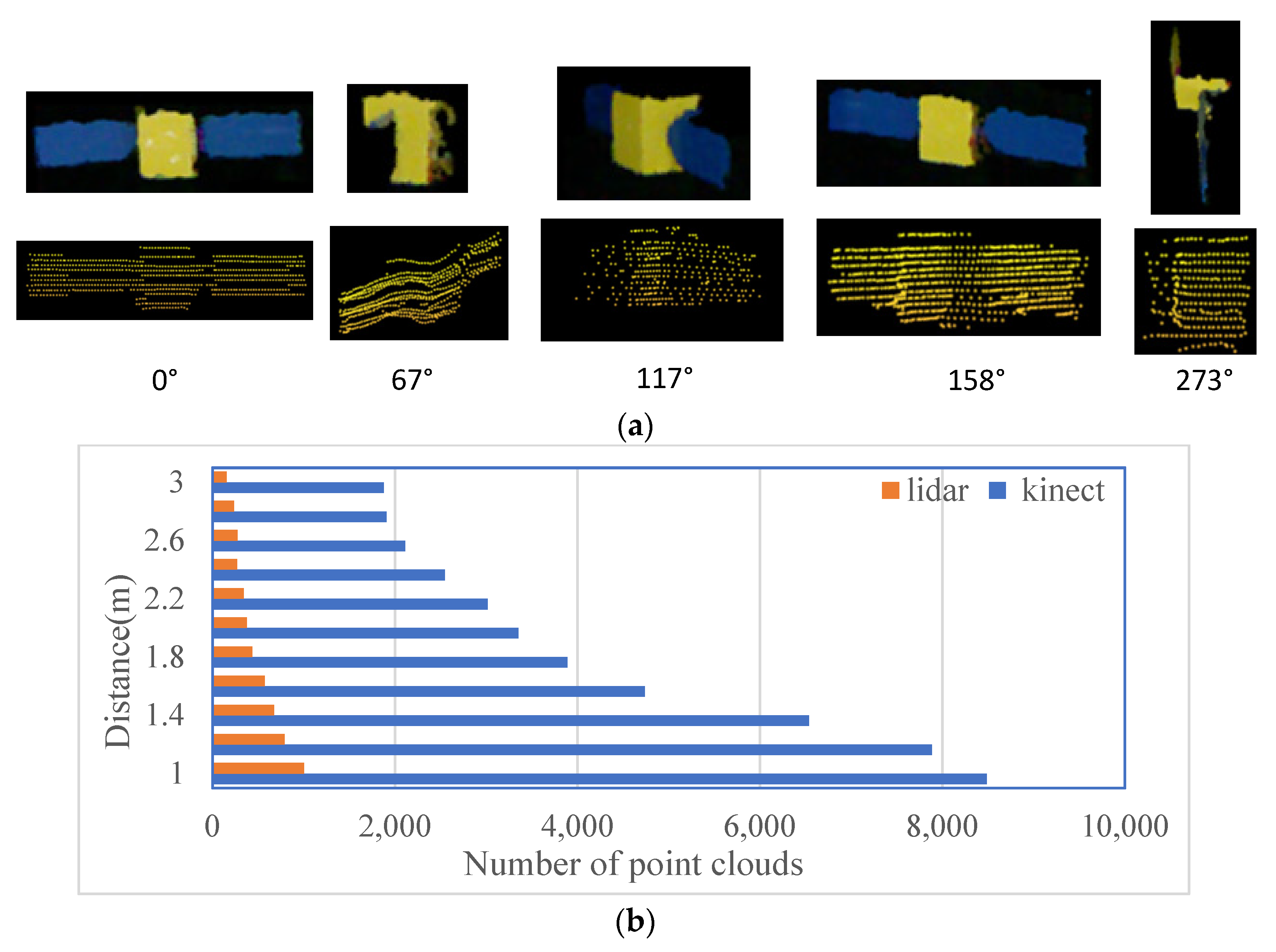
With the rapid development of high-precision sensors, such as LiDAR and Kinect sensors, point clouds have become the main data format for representing the three-dimensional world. The fusion of point clouds acquired by the same sensor is called homologous point cloud registration. However, given the complexity of the application, combining different types of sensors also combines their respective advantages; hence, it is necessary to study multi-sensor point cloud fusion, that is, cross-source fusion [20]. Owing to the dissimilar imaging mechanisms and resolutions, the density and scale of the captured point cloud also vary. Therefore, the captured point cloud may contain scale differences [21]. Figure 1a shows the Kinect and LiDAR point clouds registered at different attitudes, obtained using RS-LIDAR-32 and Kinect 1.0. Figure 1b shows a comparative histogram of the number of point clouds in a frame collected at different distances from the target. The point cloud changes from sparse to dense as the distance decreases. The number of Kinect point clouds in a frame is greater than that of LIDAR point clouds, and even at a close range of 1.2 m, the latter is very small, which makes registration difficult. The traditional feature extraction method [22,23,24] is not applicable because sparse point clouds contain few feature points. The ICP algorithm is the earliest point cloud registration algorithm [25]; it does not need to extract feature points. It requires that the two point clouds to be matched have enough corresponding points, that the registration speed is slow, and that it is easy to fall into local extreme value. More recently, many scholars have proposed various improved ICP algorithms, such as EM-ICP [26], G-ICP [27], GF-ICP [28], and kd-tree ICP [29]. These methods are not suitable for point clouds with very low overlap. NDT [30] does not require feature value extraction; instead, it optimizes the matching relationship between the two point clouds based on normal distribution transformation, which is closely related to the probability density distributions of the point clouds. The BNB-based global registration algorithm [31,32] achieves global optimal matching by setting the search boundary, and the algorithm is highly complex. The plane-based matching method proposed by Chen et al. [33] can effectively match point clouds with a low overlap rate, but it is only suitable for artificial scenes, and the confidence index is only suitable for a dedicated dataset. Cross-source point cloud registration methods based on deep learning have become an emerging topic. For instance, Huang et al. [34] designed a semi-supervised cross-source registration algorithm based on deep learning. For point clouds with a higher overlap rate, a higher matching accuracy can be achieved, and the algorithm runs faster. However, it can be seen from Figure 1 that the density of the cross-source point cloud that we studied is quite different, and the overlap rate is low.
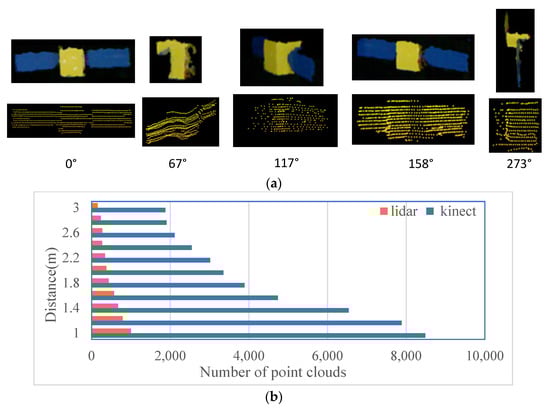
Figure 1.
(a) Comparison of Kinect (upper) and LiDAR (lower) point clouds at different rotation angles. (b) Comparison of the numbers of frame point clouds with LiDAR and Kinect at different distances.
After analyzing the above-mentioned research, we developed a point-cloud registration algorithm based on conformal geometry algebra (CGA). In this approach, the three-dimensional Euclidean space is converted into a five-dimensional conformal space. Topological operators in conformal geometric algebra can directly construct multidimensional spatial geometric elements, such as points, lines, surfaces, and spheres. Our traditional understanding of point cloud registration is that points correspond to points. However, in CGA, the concept of coordinates is abandoned, and the algorithm is no longer limited to one geometric element, but rather uses simple and unified geometric expressions in CGA to find congruent relationships between different geometric objects. For example, Cao [35] proposed a multimodal medical image registration algorithm based on the CGA feature sphere, which constructs a feature sphere from the extracted feature points to achieve sphere matching. Kleppe et al. [36] applied CGA to coarse point cloud registration. According to the curvature of the point cloud, the qualified point cloud shape distribution was determined to obtain the feature points, and the feature descriptor was constructed using the distance relationship between the point and the sphere in the CGA. However, this method requires the extraction of more feature points. The advantage of the method used in this study is that, according to the point cloud characteristics, only a few sampling points are needed to construct the rotation-invariant descriptor between the point and sphere. In the generalized homogeneous coordinate system, the objective function is constructed to obtain the best rotation and translation. To acquire the six-degree-of-freedom parameters and other motion parameters of the non-cooperative target, the algorithm we proposed in [37] is employed to obtain the point cloud contour model, using a twistor instead of a dual quaternion combined with the Clohessy–Wiltshire (CW) equation, and then uses the unscented Kalman filter (UKF) to estimate the attitudes of non-cooperative targets and improves the estimation accuracy of attitude angle. The main contributions of this study are as follows:
- (1)
- We propose a cross-source point cloud fusion algorithm, which uses the unified and simplified expression of geometric elements in conformal geometry algebra, breaks the traditional point-to-point correspondence, and constructs a matching relationship between points and spheres, to obtain the attitude transformation relationship of the two point clouds. We used the geometric meaning of the inner product in CGA to construct the similarity measurement function between the point and the sphere as the objective function.
- (2)
- To estimate the pose of a non-cooperative target, the contour model of the target needs to be reconstructed first. To improve its reconstruction accuracy, we propose a plane clustering method based CGA to eliminate point cloud diffusion after fusion. This method combines the shape factor concept and the plane growth algorithm.
- (3)
- We introduced a twist parameter for rigid body pose analysis in CGA and combined it with the Clohessy–Wiltshire equation to obtain the posture and other motion parameters of the non-cooperative target through the unscented Kalman filter.
- (4)
- We designed numerical simulation experiments and semi-physical experiments to verify our non-cooperative target measurement system. The results show that the proposed cross-source point cloud fusion algorithm effectively solves the problem of low point cloud overlap and large density distribution differences, and the fusion accuracy is higher than that of other algorithms. The attitude estimation of non-cooperative targets meets the requirement of measurement accuracy, and the estimation error of the angle of the rotating spindle is 30% lower than that of other methods.
The remainder of this paper is organized as follows. Section 2 describes in detail the non-cooperative target pose estimation method based on the proposed cross-source fusion approach. Specifically, it introduces the non-cooperative target measurement system, the proposed cross-source point cloud fusion algorithm and plane clustering method, and explains in detail the steps of the UKF algorithm based on the amount of twist. Section 3 presents the results of the numerical simulation and the semi-physical experiment and discusses the results. Section 4 discusses the value of the number of sampling points in a frame m. Finally, Section 5 summarizes the conclusions.
2. Method
2.1. Measurement System and Algorithm Framework
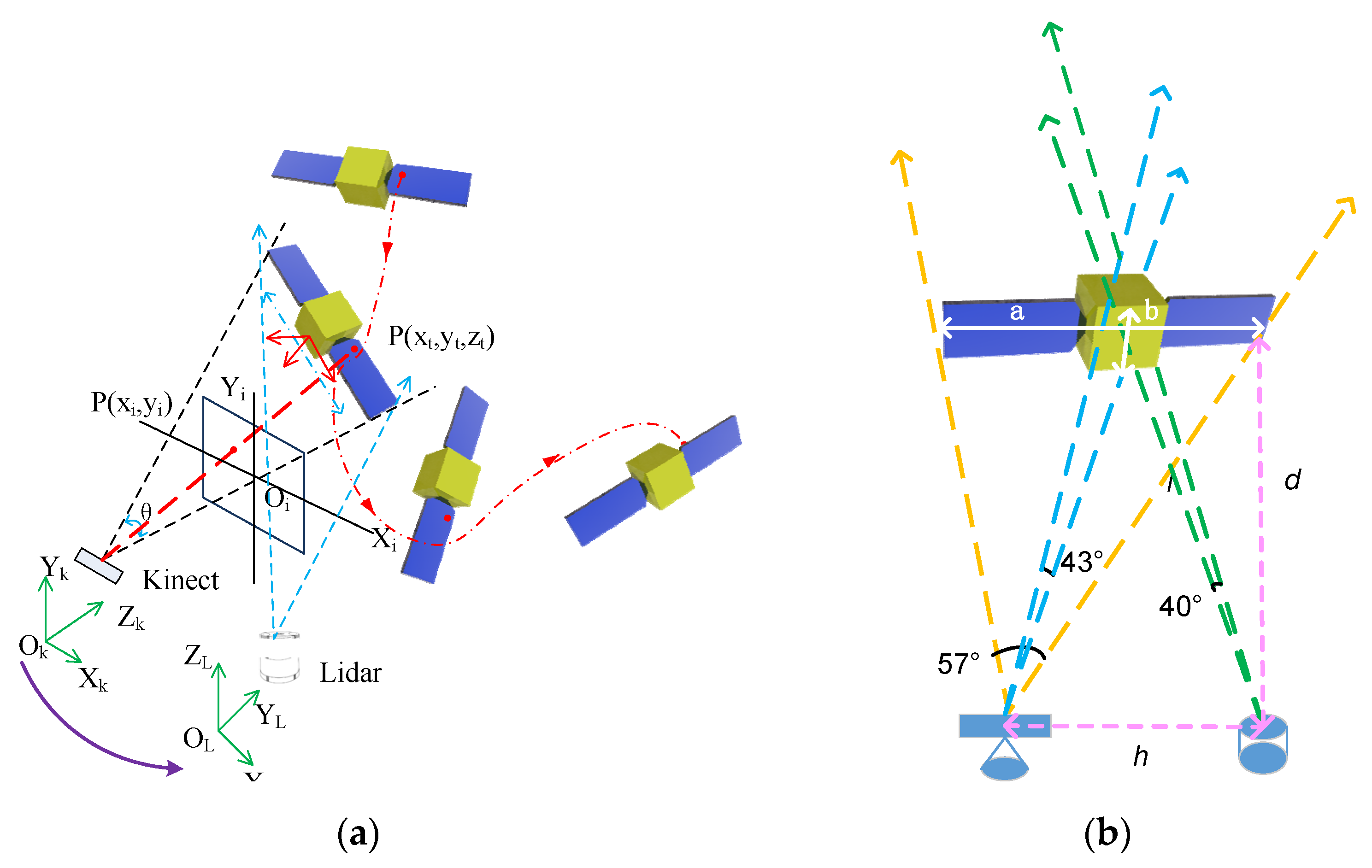
As shown in Figure 2a, the measurement system consists of a Kinect sensor, LiDAR, and a rotating satellite model. From the Figure 1, we know the Kinect point cloud has the characteristics of denseness, clear texture, and color, but it cannot be measured at long distances because of the distance limitation, even though rich point cloud information can be obtained at short distances. Some regions are shadowed from illumination, resulting in the loss of a local point cloud. LiDAR can accurately measure the distance of a point cloud; however, owing to the characteristics of the measurement instrument itself, the point cloud obtained is sparse and noisy. According to Figure 2b, we can calculate the Kinect and LiDAR measurement ranges. The Kinect has an FOV of 57° in the horizontal direction and 43° in the vertical direction. The vertical measurement angle of the LiDAR is 40°. The distance between the two sensors is h, and the distance from the sensor to the measurement target is d. Consequently, the dimensions a and b of the measurement target satisfy Equation (1).
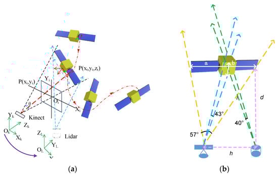
Figure 2.
(a) Measurement system. (b) Schematic diagram of the FOV for two sensors.
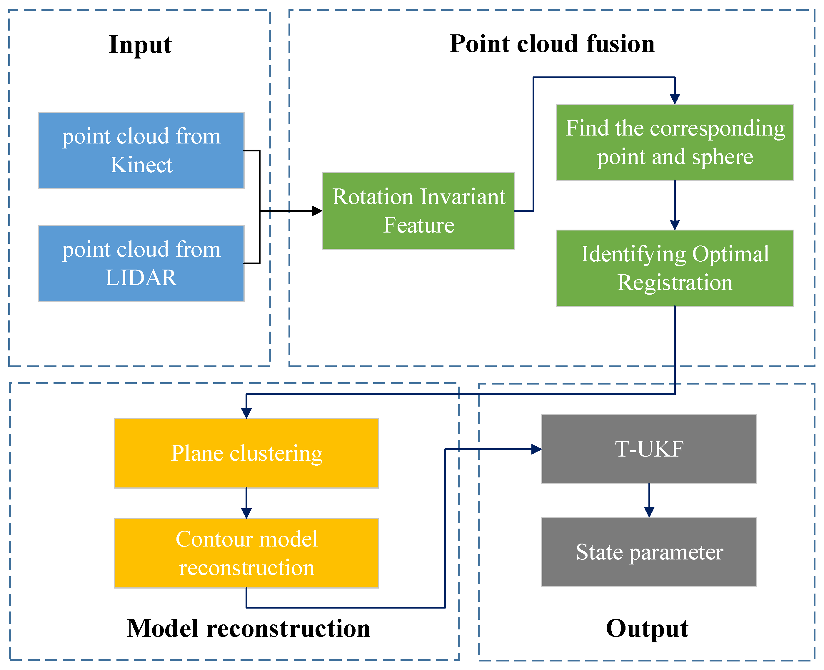
Therefore, h and d vary with the size of the measurement target. In this study, we required the measurement target to be within the FOV of the two sensors. Figure 3 shows the overall flow chart of the pose measurement system. The attitude estimation of non-cooperative spacecraft mainly involves three steps: point cloud fusion, model reconstruction, and state parameter estimation. We further explain each of these steps below.
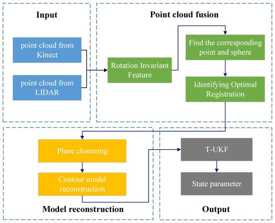
Figure 3.
Algorithm structure.
2.2. Cross-Source Point Cloud Fusion
It is well known that Kinect can record detailed structural information, but the viewing distance is limited; meanwhile, LiDAR can record distant objects, but the resolution is limited. Therefore, the point cloud fusion of different sensors provides more information and better performance in applications than the use of only one sensor type [20,38]. Point cloud fusion requires point cloud registration technology, especially when there is a large gap between the number of point clouds in a frame, as shown in Figure 1, and it is difficult to extract geometric features, so higher requirements are imposed on point cloud registration technology. This paper proposes a registration method based on CGA that can satisfy the requirements of practical applications. The conformal geometric algebra, also known as the generalized homogeneous coordinate system, was founded by Li [39]. It has become the mainstream system in international geometric algebra research. Its efficient expression and computing capabilities are favored in many scientific fields. The primary aim of the method for constructing conformal geometric algebraic space is to embed Euclidean space into high-dimensional space through nonlinear spherical projection and then to convert the high-dimensional space into conformal space through homogeneous transformation. The CGA transformation is a conformal transformation. The straight lines and planes in Euclidean space are respectively converted into circles and spheres in conformal space [40].
In CGA, the inner, outer, and geometric products are the most basic geometric operations, and the topological relationships of different geometric objects, which are constructed by the points, lines, surfaces, and volumes, are the basic geometric objects of three-dimensional Euclidean space. In conformal space, different dimensions and different types of complex spatial geometric models can be expressed by combining these objects. For example, the outer product of two points and a point at infinity in a conformal space defines a straight line L. Similarly, the outer product of three points can be used to obtain the conformal expression of a circle. The outer product expression of the plane can be obtained from the outer product of the circle and the point at infinity in the conformal space. Similarly, if the point at infinity is replaced by the ordinary conformal point, the conformal expression of the sphere can be obtained.
Under the framework of Euclidean geometry, the calculation of metrics such as the distance and angle between objects is not uniform for objects of different dimensions, and the operations between objects of different types also need to be processed separately. Consequently, traditional algorithms are complex, which is not conducive to the processing of large-scale data. The expression of geometric objects under the framework of geometric algebra has inherent and inherited geometric metric relations. For example, the inner product in space is given a clear geometric meaning that can represent the distance or angle. The ratio of the inner product between the two geometric objects to the inner product modulus is the cosine of the angle. For example, the angle between the two straight lines or two planes can be characterized by Equations (2) and (3). Table 1 shows the expression of the inner product of different geometric objects in CGA. The inner product of two points intuitively represents the inverse half of the distance between the two points. The inner product of the point and the surface is represented by the normal vector n of the plane and the distance d from the plane to the origin. The inner product between the two balls is related to the radius of the sphere. Compared to the metric operator in Euclidean space, the expressions of metrics and relations based on CGA are more concise and easier to utilize [41].
where θ represents the angle between two straight lines, or two planes, and and represent the normal vector of the plane. The symbol represents the inner product, and (·) in the all Equations used in this paper all represents the inner product.

Table 1.
Expression of the inner product of different geometric objects in CGA [42].
2.2.1. Rotation Invariant Features Based on CGA
We used the point clouds collected by LiDAR as the reference point clouds and the point clouds collected by Kinect as the mobile point clouds, denoted by and , respectively. For the rotation transformation from any point in into ,
where M is the conjugate of , which satisfies , and the rotation operator (rotor) is denoted as R. The rotation axisis a double vector, and is the rotation angle. The clockwise and axis directions are defined as positive. The translator, denoted as T, , indicates displacement.
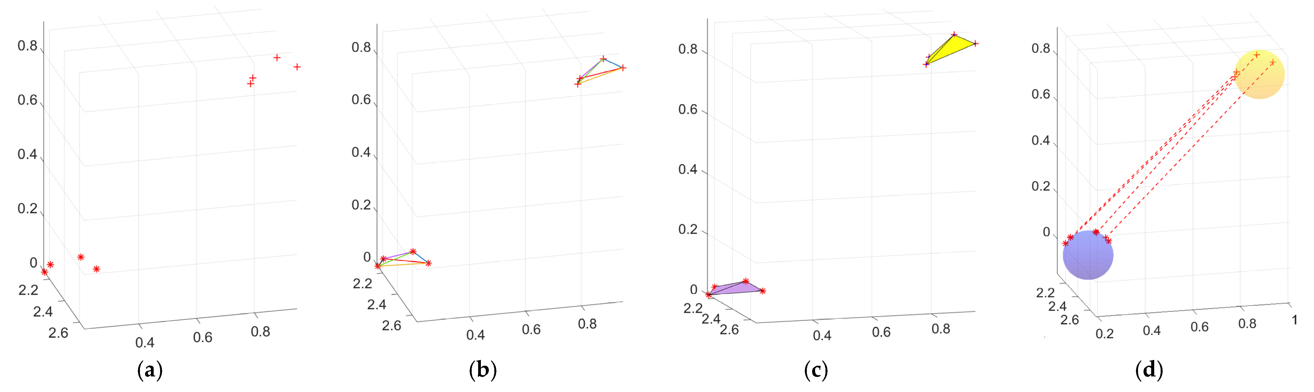
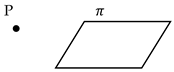
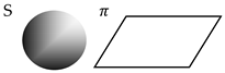
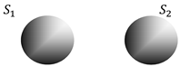
This transformation is applicable to any geometric object, including lines, planes, and bodies. Therefore, any geometric object composed of these points satisfies rotation invariance. As shown in Figure 4, the four-point pairs satisfy a certain rotation relationship. Any geometric object composed of these four points satisfies the same transformation relationship [42]:
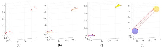
Figure 4.
Rotation-invariant features of the four geometries. (a) * means the reference point cloud, and + means the target point cloud. (b) Line segment composed of any two points . (c) Plane composed of any three points . (d) Circumscribed sphere made up of four points.
The usual registration methods are based on the registration of points and points [43], points and lines [44], points and surfaces [45], and surfaces and surfaces [33]. This report proposes a registration method for points to spheres. The distance constraint is used as a rotation-invariant feature and is employed in numerous registration algorithms. The 4PCS algorithm utilizes the invariant of the cross-ratio generated by the distance of the point pair to register [46]. The global matching algorithm proposed by Liu et al. [32] also considers the distance between two points as a rotation invariant. The distance between the lines in three-dimensional space, the distance between the surfaces, the angle between the lines, and the angle between the surfaces can also be used as feature descriptors. In CGA, the distance is represented by the inner product. The sparsity of the reference point cloud determines that it contains little geometric feature information. Therefore, the method proposed in [36] is also based on the rotation invariance of the distance between the point and the sphere. This method extracts the feature points by constructing the shape factor for each point, uses the feature points to fit the spherical surface, and constructs a descriptor of the distance between the point and the spherical surface to match the corresponding points. The method employed in this study also uses distance constraints; the difference is that we consider the distance between the point and sphere. The method proposed in this paper refers to limited sampling points in the point cloud and finds the matching feature sphere or feature circle in the moving point cloud (because the actual distribution of Kinect points has an irregular shape, feature spheres are often used). The sphere is the most basic geometry in CGA, and other geometries can be derived from it. The equation of a sphere is given by Equation (10), where O represents the center of the sphere and represents the radius. The conformal point expression of the point in the three-dimensional space is given by Equation (11). The conformal point can also be regarded as a sphere with a radius of 0, and the sphere (another expression of sphere ) can additionally be represented by four non-coplanar points , as in (10). Therefore, each sampling point corresponds to a sphere that is associated with four points. From (12), we can obtain the center and radius of the sphere [42]. Where (∙) represents the inner product.
We use the centroid of the point cloud as a reference and find four points corresponding to the inner product between the centroids in the moving point cloud. Its rotation-invariant feature satisfies (13):
where represents the inner product between two points in the reference point cloud and represents the cosine of the angle between any point and the center of mass. represents the area of a triangle formed by any three points [47].
2.2.2. Find the Corresponding Point and Sphere
We use the farthest point sampling (FPS) algorithm to sample the reference point cloud uniformly and to finally match the four points that satisfy the above formula for each sampling point in the moving point cloud. If any three of these four points are not coplanar with the fourth point, that is, , the circumscribed sphere is formed. If the points are coplanar, , a circle is formed by any three points (this article mainly uses a sphere for illustrative purposes). The cross-source point cloud registration algorithm is as follows:
- Calculate the centroids of the two point clouds and move the centroids to the origins of their respective coordinate systems: , .
- Taking the centroid as the starting point and using the farthest point sampling method, uniformly sample n points in the reference point cloud.
- Given the distance from the centroid of the reference point cloud to each sampling point, {, look for the distance to the centroid in the moving point cloud to satisfy the relationship . In this paper, T is the average distance between points of the moving point cloud.
- Use the descriptor from (13) to judge the n points sampled and retain the points that satisfy (13). Otherwise, continue sampling until the final number of retained sampling points reaches m pairs. (The value of m is discussed in Section 4 of the paper).
- According to Equations (10)–(12), construct the corresponding feature sphere in the moving point cloud and calculate the center and radius of the sphere.
2.2.3. Identifying Optimal Registration
In the previous section, we described how to find the corresponding sphere in the Kinect for the LiDAR points. Although the FPS algorithm is time-consuming, our algorithm only needs to detect a few matching point pairs. Generally, if at least three pairs of matching points are determined, the SVD decomposition method can be used to find the optimal matching relationship for the two point clouds [48,49]. In the three-dimensional Euclidean space, we use the minimum distance function (11) to represent the matching result of the two point clouds. However, because the transformation is nonhomogeneous, the calculation is difficult. In conformal space, the rotation operator M = RT is homogeneous. Therefore, (14) can be rewritten as (15). Point P can be expressed as a sphere with a radius of 0 and . The inner product represents the distance, so the distance between the two spheres can be expressed as (16), where :
In this study, we adopted the method of conformal geometric algebra, referring to the method in [50], to obtain the attitude transformation relationship between two point clouds. In CGA, we used the similarity measurement function as the objective function, as shown in Equation (17). From the above, it is evident that any geometry can be expressed as . Therefore, this function describes the similarity between all the geometric bodies:
where the symbol ℶ represents symmetry and satisfies ; consequently, . represents the weight. In our algorithm, represents the feature point in the reference point cloud and represents the feature ball in the corresponding moving point cloud. Therefore, our similarity measurement function can be expressed as (18), where :
The basis vector of R is , and the basis vector of T is [51]. Due to
the eigenvector corresponding to the largest eigenvalue of is, and the rotation matrix can then be calculated using Equation (20).
Similarly, and can be decomposed into sub-matrices . Next, we can calculate , where is the pseudo-inverse matrix of (Moore-Penrose pseudoinverse). T is given by Equation (21), and the optimization we are looking for is .
2.3. Point Cloud Model Reconstruction
In this step, it is necessary to perform a three-dimensional reconstruction of the fused point cloud. In this section, we use the method proposed in our previous article [37] to obtain the outer contour model of the non-cooperative target to estimate the pose and motion parameters of the non-cooperative target in the next step. In that study [37], we proposed a new point cloud contour extraction algorithm and obtained the contour model of the non-cooperative target through multi-view registration-based ICP. However, in this study, the reconstructed object is a frame point cloud after the fusion of two sensors. As shown in Figure 5a, the point cloud distribution obtained by the fusion algorithm is rather scattered. Consequently, the point cloud density varies greatly at the edge, which affects the accuracy of model reconstruction. Therefore, in this study, we propose a plane clustering method to eliminate point cloud diffusion. This method combines the shape factor concept proposed in [52,53,54] with the plane growth algorithm. Because the number of Kinect point clouds in the frame is large and the distribution is dense, the shape factor of the Kinect point cloud (denoted as in what follows) is extracted and the LiDAR point cloud (denoted as in what follows) is clustered to the nearest plane.
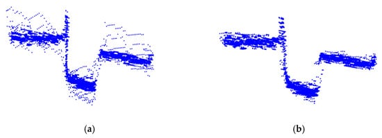
Figure 5.
Point cloud (a) before clustering and (b) after clustering.
First, for each point in , we find the covariance matrix in its neighborhood and its corresponding eigenvalue , eigenvector , and normal vector . The shape factors represent linear, planar, and spherical shapes, respectively. The calculation formula is given by Equation (22):
where , , and represent the eigenvalues arranged in descending order, . When any one of is much larger than the other two, the K-neighborhood of this point conforms to its corresponding shape distribution. If there are two larger shape factors , then this point is the edge point of the plane. The highest number of Kinect point clouds we obtained conformed to two distributions: linear and planar. Therefore, we only considered these two cases in this study. When the K-neighboring points of any point in are arranged in order of ascending distance, and when these points all satisfy a shape distribution at the same time, we consider these points to be collinear or coplanar. These points can be fitted to a straight line or plane . The definitions of a straight line and plane in CGA are given by Equations (23) and (24), respectively:
where and are two points on a straight line. The value is the normal vector of plane , and is the distance from plane to the origin.
When a point in and the line or plane closest to it meet the judgment condition of Equation (25), the projection point of the point in on is obtained according to Equation (26). Otherwise, we consider this point to be a noise point, which can be eliminated:
In particular, is a point in and is a point in . represents the straight line closest to in the point cloud, and represents the plane closest to in the point cloud. The valuerepresents the normal vector of the center point of or , and represents the normal vector of a point in . The value is the normal vector angle threshold, and is twice the distance between two adjacent planes in . Figure 5b shows the results of the point cloud fusion using the plane-clustering algorithm.
2.4. Estimation of Attitude and Motion Parameters
Through the reconstruction of the contour model, the relative pose estimation of the point cloud between consecutive frames can be obtained. It is also necessary to predict the centroid position, motion speed, and angular velocity to estimate the motion state of a non-cooperative target. In addition, it is beneficial to capture tasks. Because of the singularity of Euler angles, quaternions are frequently used, since their kinematic equations are linear. In particular, the attitude description of the Kalman filter [55] prediction step is important in spacecraft attitude control systems. Most previous researchers have used the extended Kalman filter (EKF) method to estimate the relative attitude, the position motion parameters, and the moment of inertia [56,57,58,59]. When dealing with the nonlinear problems of dynamic and observation models, the UKF can achieve the same accuracy as the EKF [60], but when the peak and high-order moments of the state error distribution are prominent, the UKF can yield more accurate estimations. Conformal geometric algebra can provide an effective method of dealing with three-dimensional rigid body motion problems [61,62]. The rigid body motion equation described by CGA is consistent with the dual quaternion rigid body motion equation. The author [63] proposed a six-dimensional twistor to model the rotation and translation integrally without unitization constraints. In this study, we used a twistor combined with the CW equation and applied the UKF to estimate the motion parameters of non-cooperative targets.
The state equation described by the pose dual quaternion is
where represents the translation vector of the target, represents the linear velocity of the movement, , and represents the angular velocity. Equation (28) is then employed to obtain the expression of the dual quaternion of the pose:
Because the unitization constraint cannot be guaranteed when the pose dual quaternion is used in the UKF to generate sigma points, we use the twist as the error pose orbit state parameter to generate sample points [64]. The twist representation is the Lie algebra representation. The parameterized space of the rigid body motion given by it is a vector space, which is very beneficial for parameter optimization [61]. The twist error corresponding to the dual quaternion error is given in (29), and the corresponding covariance matrix is, where is the dual quaternion error and represents quaternion multiplication:
Construct sigma sample points with error twistor:
The weight is , where L is the dimension of the state quantity and . After obtaining the sample points of the twist error, the inverse transformation of the twist is used to obtain the corresponding sample points of the dual quaternion error , and the pose dual quaternion (36) and predicted point are obtained through the state equation:
When the state propagation time interval is sufficiently small and the angular velocity is constant, the state propagation equation of the pose dual quaternion is:
The CW equation [65] can be used to obtain the kinematic equation of the centroid offset position:
where is the gravitational constant .
The observation Equation (40) can be used to generate the observation points of the predicted points. In this study, the observation pointof the pose dual quaternion and observation position were constructed through the model reconstruction:
The Algorithm 1 flow for using the UKF [64] for pose and motion parameter estimation is as follows:
| Algorithm 1. UKF Algorithm | |
| Input: | State variable at time k , covariance matrix |
| Output: | At time k+1 , |
| Initial value: | , |
| Iteration process | |
| Step 1: | Convert the pose quaternion into the error twistor , and perform sigma sampling on it |
| Step 2: | Convert the sigma sample point of the error twistor into a pose dual quaternion, and obtain a new prediction point through the state equation |
| Step 3: | Determine the mean and covariance of the predicted points , , and |
| Step 4: | Obtain the new observation point mean and covariance through the observation equations , , and |
| Step 5: | Determine the Kalman gain for the UKF using and |
| Step 6: | Update the status according to and |
3. Experimental Results and Analysis
To verify the CGA-based cross-source point cloud fusion algorithm proposed in this study, numerical simulation experiments and semi-physical experiments were conducted.
3.1. Numerical Simulation
The CGA-based cross-source point cloud fusion algorithm proposed in this paper served as the basis for pose estimation and was also the core of this study. We used Blendor software to generate satellite point clouds [66] and verified the proposed algorithm according to the following approach.
- Step 1:
- Set the positions of the Kinect and LiDAR sensors in the Blendor software, and select the appropriate sensor parameters. Table 2 lists the sensor parameter settings for the numerical simulation in this study.
Table 2. Kinect and LIDAR parameters in the numerical simulation experiment.
- Step 2:
- Rotate the satellite model once around the z axis (inertial coordinate system), and collect 16 frames of point cloud in 22.5° yaw angle increments.
- Step 3:
- Use the proposed fusion algorithm to register the point clouds collected by the two sensors.
- Step 4:
- Rotate the satellite model around the x axis or y axis, and repeat steps 2–4.
- Step 5:
- Adjust the distance between the two sensors and the satellite model, and repeat steps 2–5.
- Step 6:
- Use the root mean square error (RMSE) to verify the effectiveness of the algorithm.
3.1.1. Registration Results
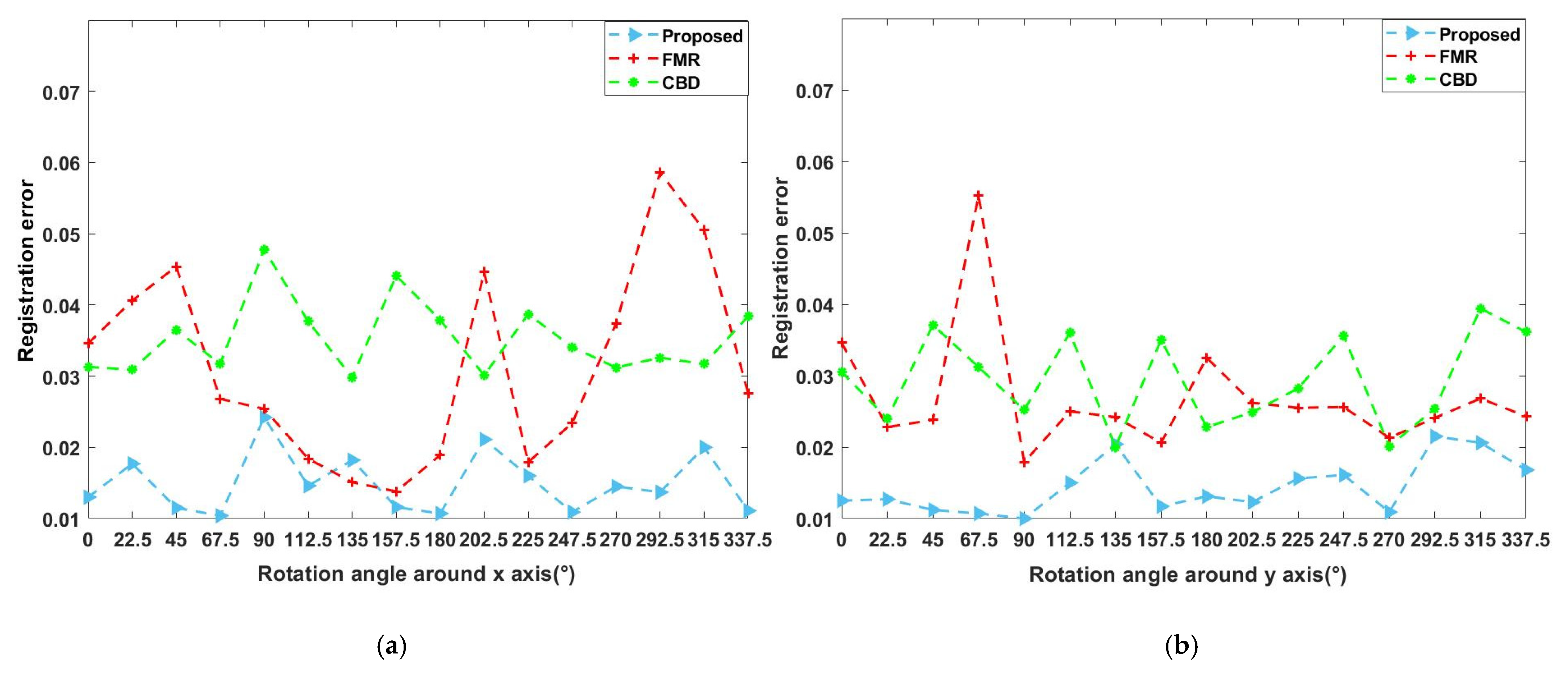
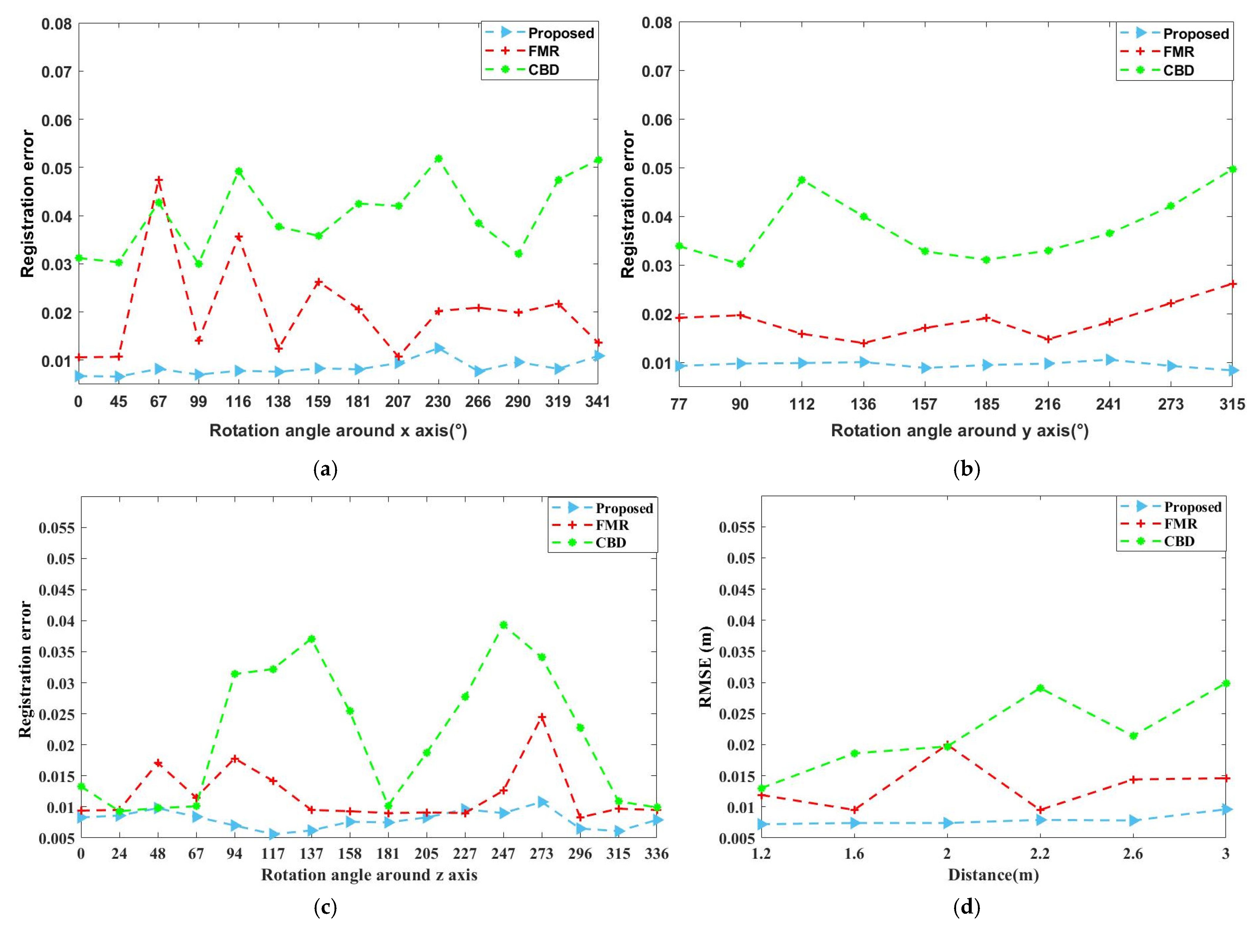
In the numerical simulation experiment, we set six distances between the non-cooperative target and the service spacecraft. At each distance, 16 groups of point clouds around the x axis, y axis, and z axis of the non-cooperative target were obtained respectively. At each distance, we obtained 48 sets of point cloud data to evaluate the root mean square error at each distance. We compared the cross-source point cloud fusion algorithm (FMR) based on the deep learning technique in [34] and the curvature-based registration algorithm (CBD) in [36] with the algorithm proposed in this paper. Figure 6a–c shows the errors of the three methods for point cloud fusion with different attitude angles when the non-cooperative target rotates around the x, y, and z axes. From the figure, it can be implied that irrespective of the type of axis around which the target rotates, our method is optimal. Figure 6d shows the root mean square error of the three algorithms at different distances when the serving spacecraft approaches the non-cooperative target from far to near. This experiment verifies that our algorithm has a high matching accuracy and robustness.
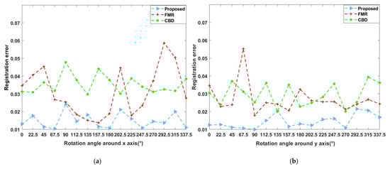
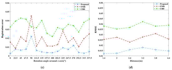
Figure 6.
(a–c) When rotating around the x axis, y axis, and z axis, simulated point cloud fusion error for different rotation angles. (d) RMSE change curve for registration at different distances.
3.1.2. Pose Estimation Results of Simulated Point Clouds
In this study, we used the method proposed in our previous study [37] to obtain a 3D contour model of the non-cooperative target. Figure 7 shows the three-dimensional views of the reconstructed 3D satellite model.
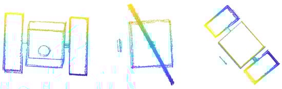
Figure 7.
Simulated point cloud contour model.
For the point cloud obtained from the simulations, the following pose estimation method was used. We set the target to rotate around the z axis at a speed of 5°/s. The initial parameters were set by the software, as shown in Table 3. Except for the Euler angle that changed with the target rotation, the initial and final parameters were the same.
Table 3.
Initial parameters set in the numerical simulation experiment.
In Figure 8a,c, the blue and red curves represents the result of pose estimation and true values, respectively. In the simulation experiment, the maximum error between the translational position of the target along the x, y, and z axes and the true value was 0.16, 0.02, and 0.08, respectively. The speed error along each of the three axes was less than 0.05. Figure 8b,d depicts the errors between the attitude angle and angular velocity. The results indicate that the attitude angle errors along the x and y axes were less than 0.3°. Notably, the target was rotated around the z axis, making the point cloud change in this direction very clearly. The error around the z axis was less than 1°. In addition, the angular velocity error along the x and y axes was less than 0.001°.
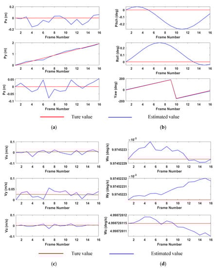
Figure 8.
(a) Translational position, (b) angular position, (c) velocity, and (d) angular velocity estimation results of the target spacecraft.
3.2. Semi-Physical Experiment and Analysis
Because the point cloud generated by the software is dense, the distribution is regular and there is little noise. However, in fact, the point cloud collected by our sensors was irregularly distributed and sparse. We simulated the rotation of non-cooperative targets in space in the laboratory, employed sensors to collect point clouds, used the method proposed in this article for registration, and finally determined the pose and motion parameters.
3.2.1. Experimental Environment Setup
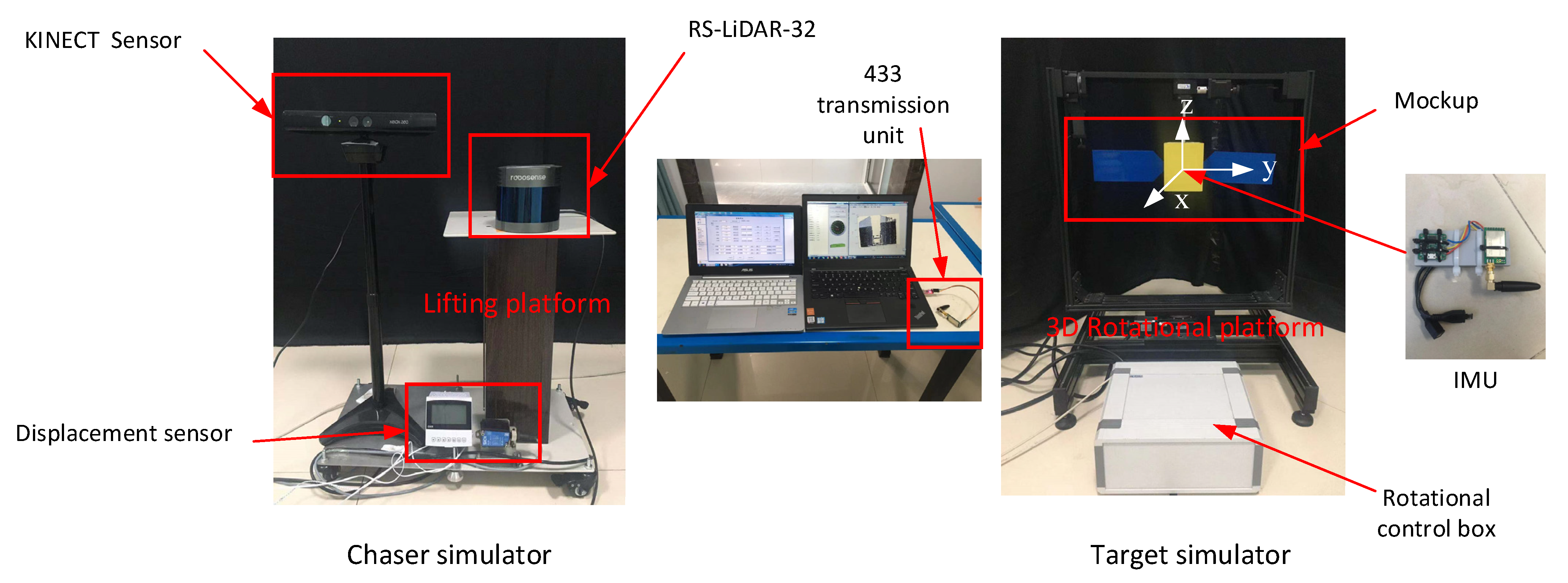
To test the performance of the proposed estimation algorithm further, a semi-physical experiment was conducted. As shown in Figure 9, the satellite model was used as a non-cooperative spacecraft, a three-dimensional rotating platform was used to simulate the motion of the non-cooperative spacecraft, and a self-made flatbed was utilized instead of the chasing spacecraft. We installed a lifting platform on the chasing spacecraft to control the position of the LiDAR. A Kinect was installed on a lifting bracket, and a displacement sensor was installed under the chasing spacecraft. By adjusting the distance from the LiDAR to the ground, we ensured that the target was in the FOV of the LiDAR. The three-dimensional rotating table was controlled using a control box to adjust its movement in space. The speed of the rotating table was 5°/s, and all three axes could rotate at a uniform speed. An IMU was installed in the main box of the non-cooperative target to transmit the true attitude angle and motion parameters of the target back to the personal computer through the 433 wireless communication module. Table 4 and Table 5 list the parameters of the Kinect and LiDAR sensors used in this experiment.
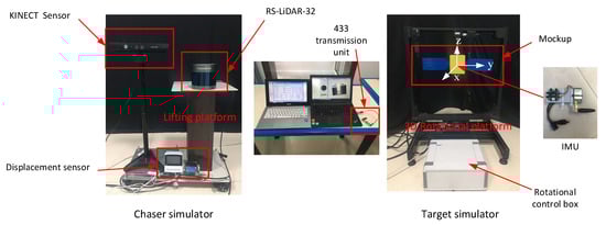
Figure 9.
Experimental device for simulating the relative motion between the spacecraft and target spacecraft.
Table 4.
Kinect 1.0 specifications.
Table 5.
RS-LiDAR-32 specifications.
3.2.2. Results of Semi-Physical Experiments
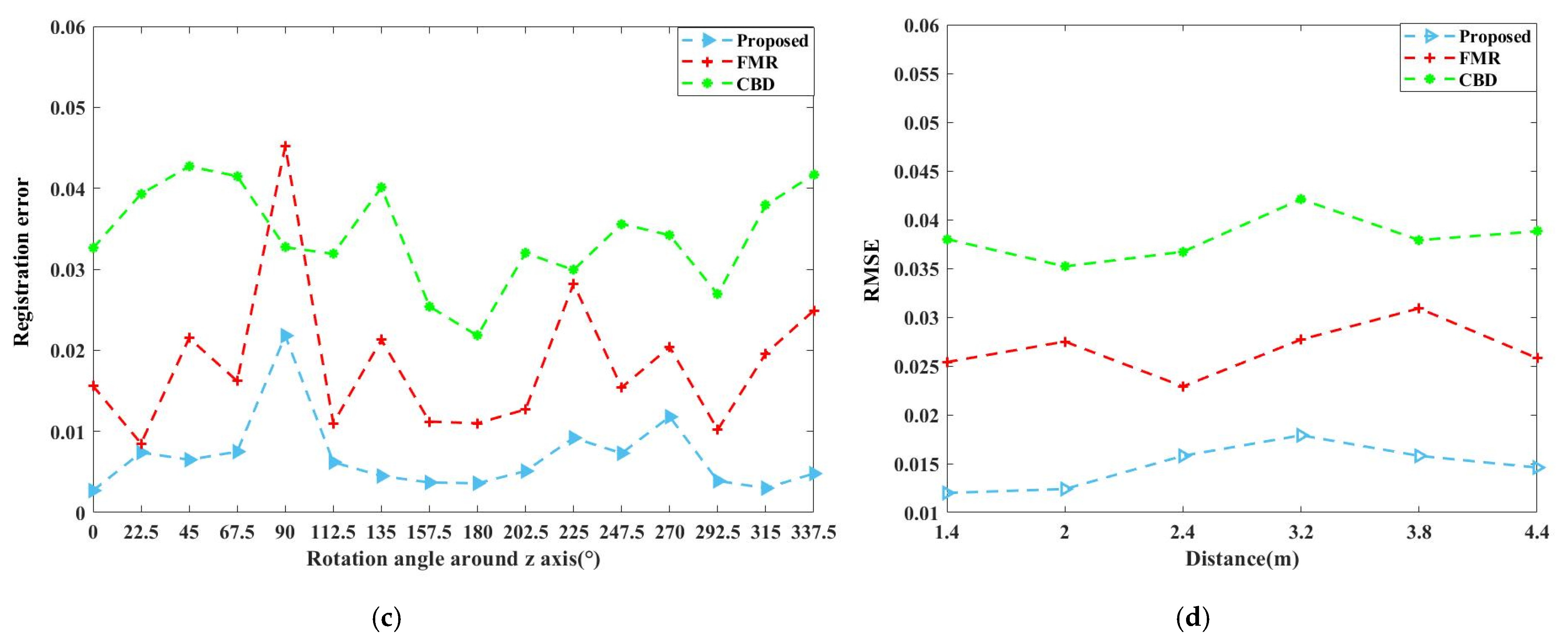
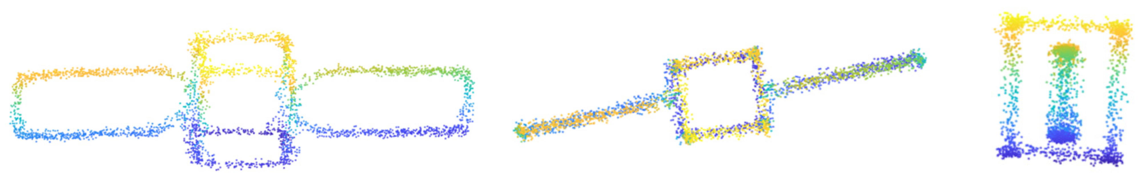
In the semi-physical simulation, we also set six distances, as well as, 14, 10, and 16 sets of point cloud at each distance for the target spacecraft rotating around the x axis, y axis, and z axis, respectively. Figure 10a–c shows the point cloud fusion error under different rotation attitudes collected by the two sensors when the target spacecraft rotates around different axes. Each distance corresponds to 40 sets of point cloud. Figure 10d shows the RMSE of the point cloud registration at different distances obtained when the service spacecraft approaches the target spacecraft. We compared the accuracy of the proposed algorithm with the other two algorithms [34,36], and the results reveal that the proposed algorithm had the smallest error. Figure 11 demonstrates the results of using the cross-source point cloud fusion algorithm proposed in this study at different poses. It can be seen that even at a very low overlap rate, our algorithm still showed strong robustness. Figure 12 shows the 3D contour model of the non-cooperative target. The overall structure can be clearly identified, which proves the effectiveness of our algorithm.
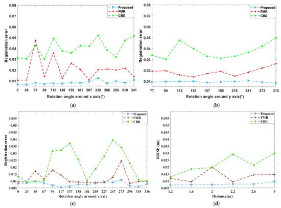
Figure 10.
(a–c) When rotating around the x axis, y axis, and z axis, real point cloud fusion error for different rotation angles. (d) RMSE change curve for registration at different distances.
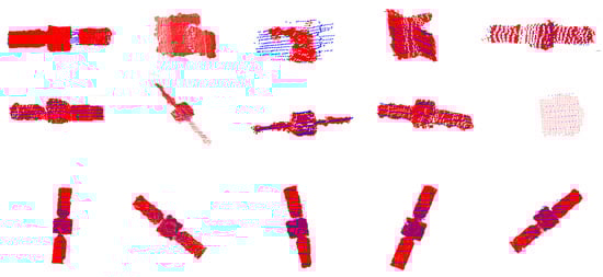
Figure 11.
Results of point cloud fusion at different poses.
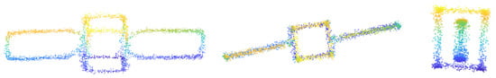
Figure 12.
Contour model of the target spacecraft.
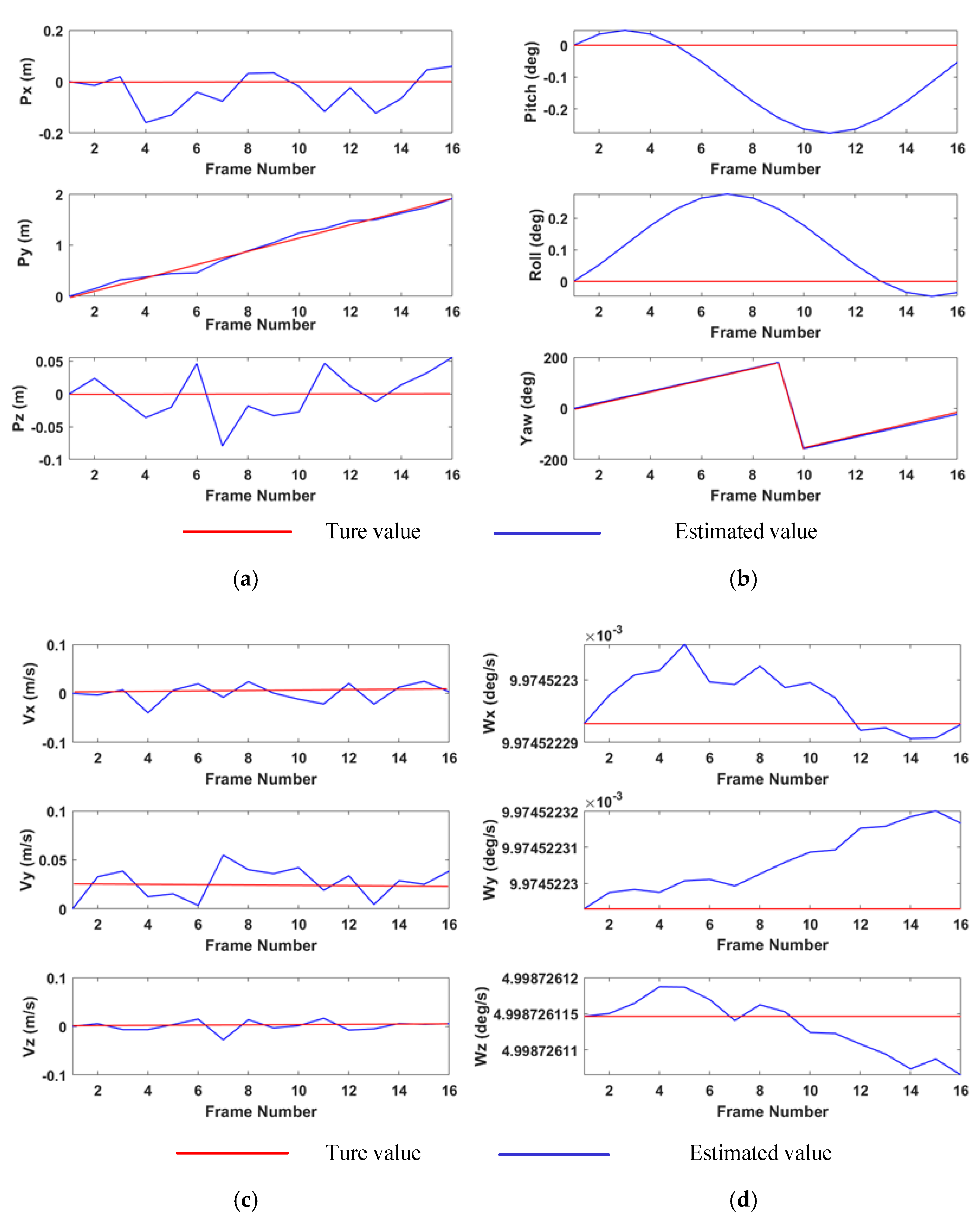
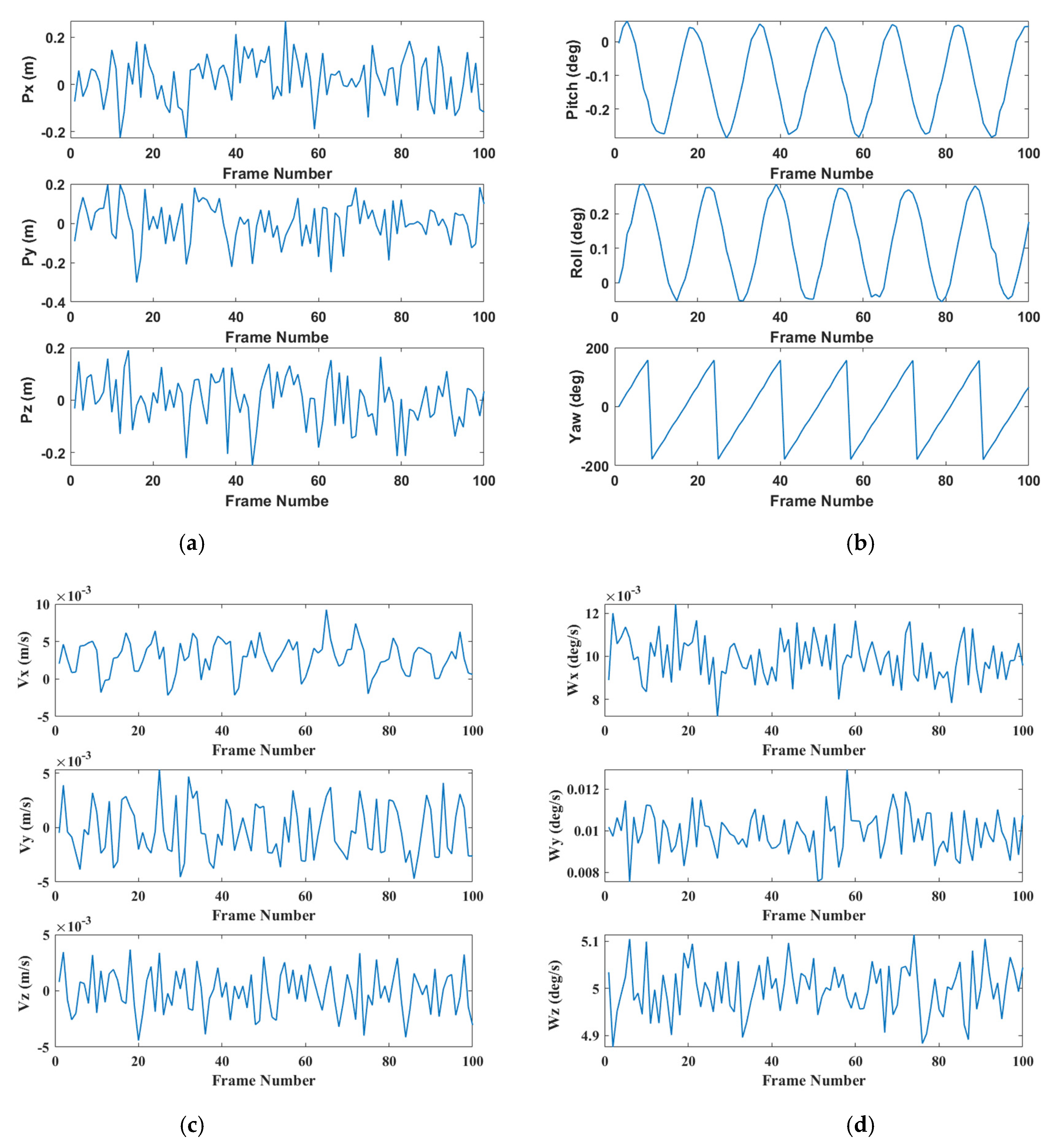
Figure 13a–d presents the results of the translational position estimation, Euler angle estimation, velocity estimation, and angular velocity estimation of the target obtained by the proposed method, respectively. In our semi-physical experiment, the target was rotated clockwise around the z axis, the sampling interval was approximately 22.5°, and the number of sampling frames was 100. Although the initial position of the rotating platform was set to (0, 0, 0) m and the initial rotation angle was (0, 0, 0)°, the position of the mass center of the target spacecraft did not change visually. However, because the target spacecraft was connected to the rotating table, there were errors in the angle and translational positions of the rotating table during the continuous rotation process. Through the IMU, we indeed detected that the target spacecraft had a linear acceleration of ±0.0002. Therefore, the velocity in the x direction was no longer 0, and there was a displacement change between frames 40 and 60, but it quickly converged.

Figure 13.
Non-cooperative target pose estimation results of our method: (a) translational position, (b) rotational position, (c) velocity, and (d) angular velocity estimation results.
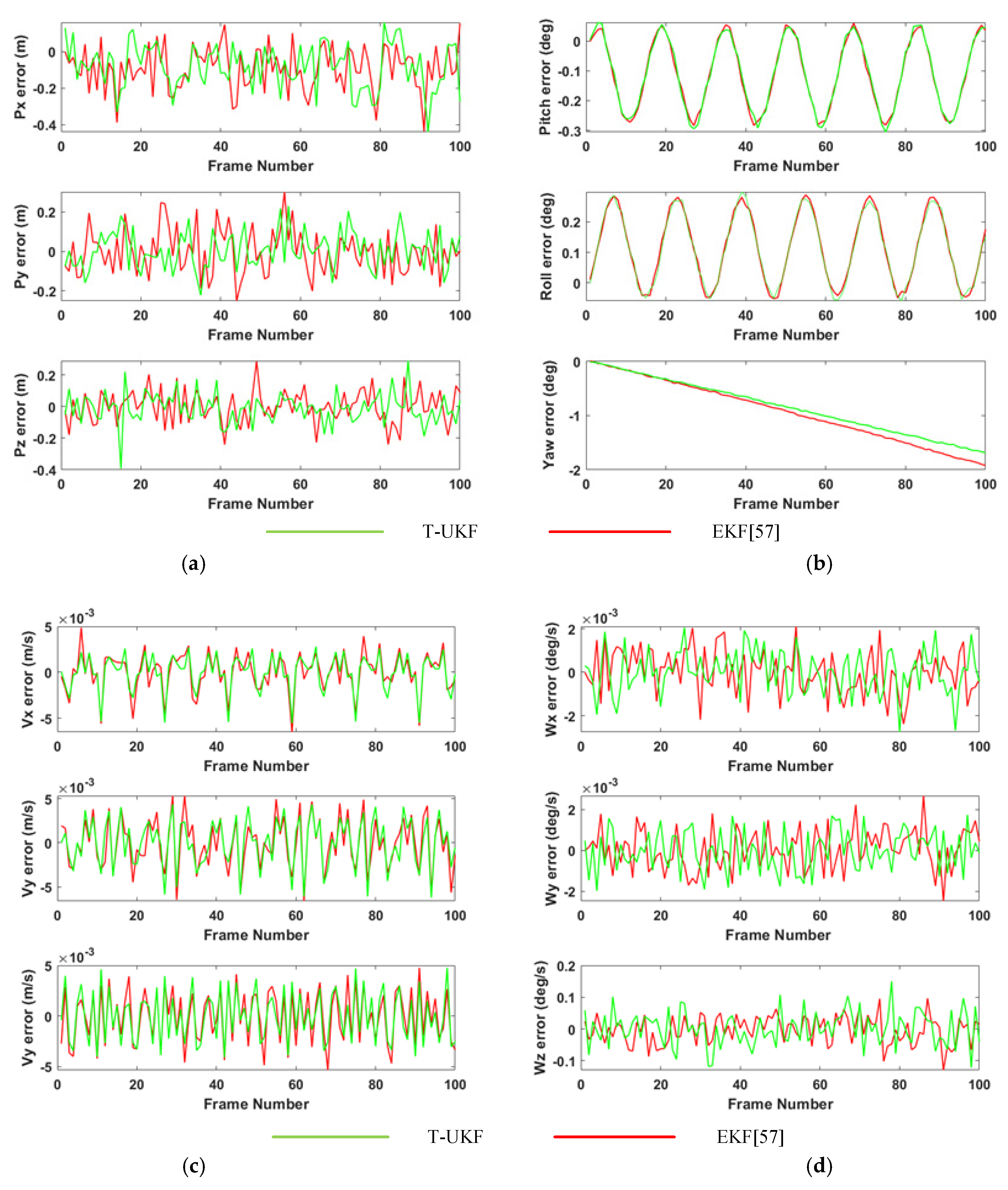
Figure 14a–d compares the errors between the attitude estimation and the true values of the parameters obtained by the proposed algorithm and the quaternion-based EKF algorithm [57] (the true value was determined based on the IMU supply). The translational position estimation error along the x, y, and z axes for these algorithms, m, was less than 0.3 m; the linear velocity estimation error along the x, y, and z axes was less than 0.01 m/s; the angular velocity estimation error was less than 0.1°/s; and the estimated errors of the three parameters obtained by these two methods were the same. However, the error of the Euler angle (yaw angle) acquired using the twist-based UKF method in this study was 30% lower than in previous studies [57]. Therefore, the proposed algorithm yields attitude angle estimations close to the true value.
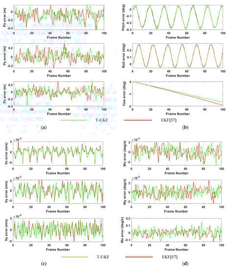
Figure 14.
Comparison of the (a) translational position, (b) rotation angle, (c) velocity, and (d) angular velocity estimation errors of the proposed algorithm and a previously reported algorithm [57].
4. Discussion
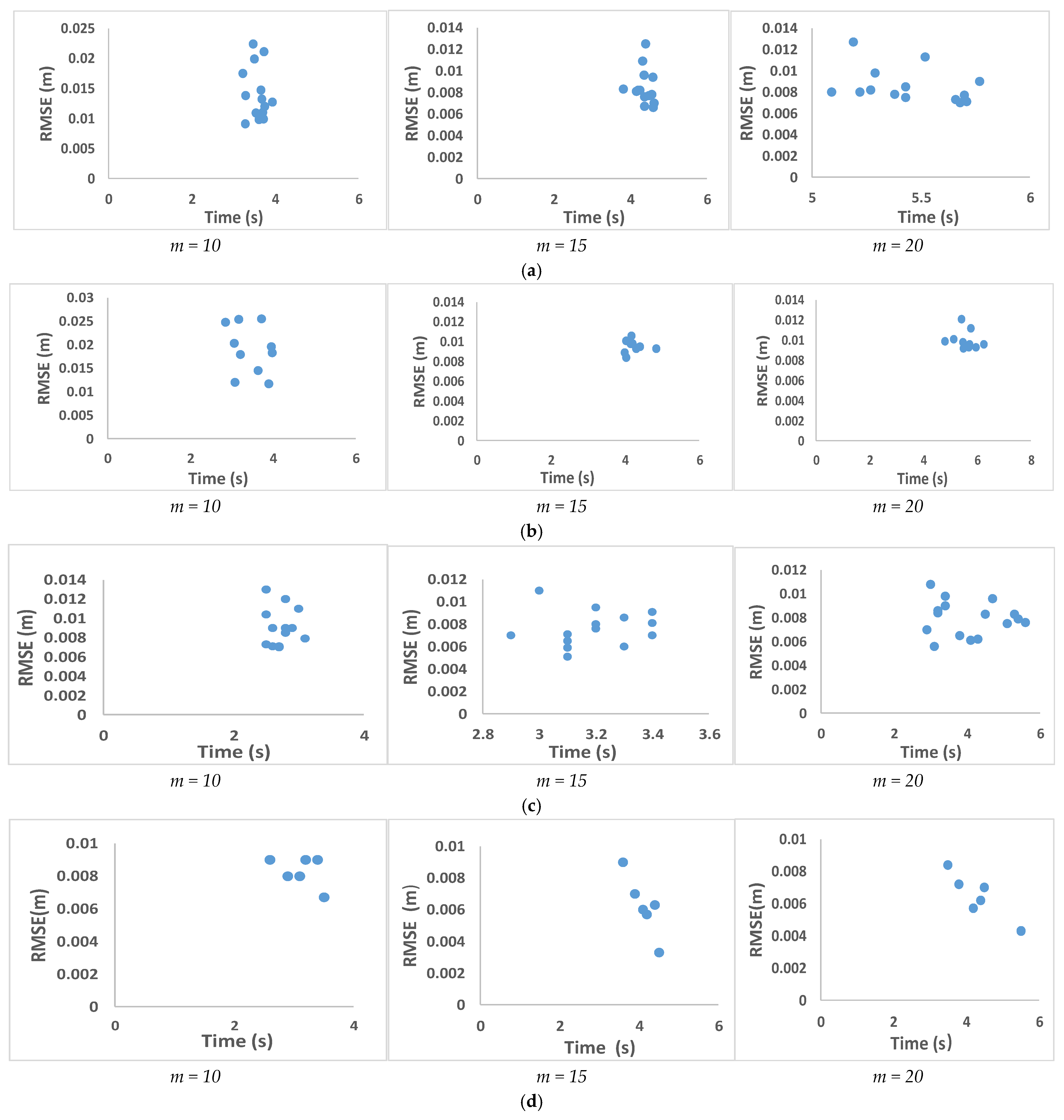
In this section, we discuss the value of the sampling point m mentioned in the cross-source point-cloud fusion algorithm. In the proposed approach, the FPS algorithm is used to sample the reference point cloud to ensure that the sampling points are as evenly distributed on the reference point cloud as possible to achieve global registration. The execution time of the algorithm is related to the number of sampling points m. Figure 15a–c shows the relationship between RMSE of the cross-source point cloud fusion algorithm and the running time with different values of m, when the non-cooperative target uses the x, y, and z axis, respectively, as the main axis of rotation. Figure 15d shows the relationship between the RMSE and the running time of the cross-source point cloud fusion algorithm when m takes different values at different distances. We can see that when , the algorithm consumes less time, but the error is greater. When , the algorithm time increases, but the registration error does not change significantly compared to that in the case of . Therefore, as a compromise, m was set to 15 for this paper.
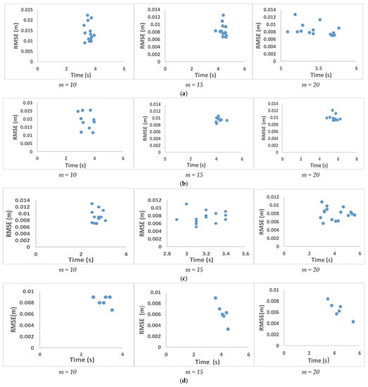
Figure 15.
(a–c) The x axis, y axis, and z axis, respectively, as the main axis of rotation, time and RMSE variation of different rotation attitudes. (d) Time and error changes when the service spacecraft approaches from far to near.
The cross-source point cloud fusion algorithm proposed in this paper has a higher accuracy than the other two algorithms [34,36]. The number of point clouds in a frame obtained at different distances is quite different. In the semi-physical experiment, we collected 40 frames of point cloud for each distance. Table 6 shows the average number of point cloud in a frame at different distances, and the average running time of the point cloud fusion algorithm at each distance. Table 6 shows that as the number of point clouds in a frame increases, our algorithm does not lag behind in terms of time.
Table 6.
Algorithm average running time.
5. Conclusions
A non-cooperative target pose measurement system fused with multi-source sensors was designed in this study. First, the cross-source point cloud fusion algorithm-based CGA was proposed. This method used the unified and simplified expression of geometric elements, and the geometric meaning of the inner product in CGA constructed the matching relationship between points and spheres and the similarity measurement objective function. Second, we proposed a plane clustering algorithm of point cloud, in order to solve the problem of point cloud diffusion after fusion, and the method proposed in [37] was used to obtain the model reconstruction of non-cooperative targets. Finally, we used the twistor along with the Clohessy–Wiltshire equation to obtain the posture and other motion parameters of the non-cooperative target through the unscented Kalman filter. The results of the numerical simulation and the semi-physical experiment show that the proposed measurement system meets the requirements for non-cooperative target measurement accuracy, and the estimation error of the angle of the rotating spindle was found to be 30% lower than that of other methods. The proposed cross-source point cloud fusion algorithm can achieve high registration accuracies for point clouds with different densities and small overlap rates.
To achieve a seamless connection between long- and short-distance measurements, multi-sensor data fusion is the main research direction for the future. Our future work will focus on non-cooperative target measurement based on cross-source point cloud fusion within the framework of deep learning.
Author Contributions
Conceptualization, J.L.; methodology, J.L.; software, J.L.; validation, J.L., Q.P. and Y.Z.; formal analysis, L.Z.; investigation, Q.P.; resources, L.Z.; data curation, J.L.; writing—original draft preparation, J.L.; writing—review and editing, Y.Z.; visualization, Q.P.; supervision, Y.Z.; project administration, Y.Z.; funding acquisition, Q.P. All authors have read and agreed to the published version of the manuscript.
Funding
This article was supported by “the National 111 Center”.
Data Availability Statement
Data available on request to the authors.
Acknowledgments
The authors would like to thanks the Trans-power Hydraulic Engineering Xi’an Co., Limited (China) for providing us with the laboratory.
Conflicts of Interest
The authors declare no conflict of interest.
References
- Zhao, P.; Liu, J.; Wu, C. Survey on research and development of on-orbit active debris removal methods. Sci. China Ser. E Technol. Sci. 2020, 63, 2188–2210. [Google Scholar] [CrossRef]
- Ding, X.; Wang, Y.; Wang, Y.; Xu, K. A review of structures, verification, and calibration technologies of space robotic systems for on-orbit servicing. Sci. China Ser. E Technol. Sci. 2021, 64, 462–480. [Google Scholar] [CrossRef]
- Opromolla, R.; Fasano, G.; Rufino, G.; Grassi, M. A review of cooperative and uncooperative spacecraft pose determination techniques for close-proximity operations. Prog. Aerosp. Sci. 2017, 93, 53–72. [Google Scholar] [CrossRef]
- Yingying, G.; Li, W. Fast-swirl space non-cooperative target spin state measurements based on a monocular camera. Acta Astronaut. 2019, 166, 156–161. [Google Scholar] [CrossRef]
- Vincenzo, C.; Kyunam, K.; Alexei, H.; Soon-Jo, C. Monocular-based pose determination of uncooperative space objects. Acta Astronaut. 2020, 166, 493–506. [Google Scholar] [CrossRef]
- Cassinis, L.P.; Fonod, R.; Gill, E.; Ahrns, I.; Gil-Fernández, J. Evaluation of tightly- and loosely-coupled approaches in CNN-based pose estimation systems for uncooperative spacecraft. Acta Astronaut. 2021, 182, 189–202. [Google Scholar] [CrossRef]
- Yin, F.; Wusheng, C.; Wu, Y.; Yang, G.; Xu, S. Sparse Unorganized Point Cloud Based Relative Pose Estimation for Uncooperative Space Target. Sensors 2018, 18, 1009. [Google Scholar] [CrossRef]
- Lim, T.W.; Oestreich, C.E. Model-free pose estimation using point cloud data. Acta Astronaut. 2019, 165, 298–311. [Google Scholar] [CrossRef]
- Nocerino, A.; Opromolla, R.; Fasano, G.; Grassi, M. LIDAR-based multi-step approach for relative state and inertia parameters determination of an uncooperative target. Acta Astronaut. 2021, 181, 662–678. [Google Scholar] [CrossRef]
- Zhao, D.; Sun, C.; Zhu, Z.; Wan, W.; Zheng, Z.; Yuan, J. Multi-spacecraft collaborative attitude determination of space tumbling target with experimental verification. Acta Astronaut. 2021, 185, 1–13. [Google Scholar] [CrossRef]
- Masson, A.; Haskamp, C.; Ahrns, I.; Brochard, R.; Duteis, P.; Kanani, K.; Delage, R. Airbus DS Vision Based Navigation solutions tested on LIRIS experiment data. J. Br. Interplanet. Soc. 2017, 70, 152–159. [Google Scholar]
- Perfetto, D.M.; Opromolla, R.; Grassi, M.; Schmitt, C. LIDAR-based model reconstruction for spacecraft pose determination. In Proceedings of the 2019 IEEE 5th International Workshop on Metrology for AeroSpace (MetroAeroSpace), Torino, Italy, 19–21 June 2019. [Google Scholar]
- Wang, Q.L.; Li, J.Y.; Shen, H.K.; Song, T.T.; Ma, Y.X. Research of Multi-Sensor Data Fusion Based on Binocular Vision Sensor and Laser Range Sensor. Key Eng. Mater. 2016, 693, 1397–1404. [Google Scholar] [CrossRef]
- Ordóñez, C.; Arias, P.; Herráez, J.; Rodriguez, J.; Martín, M.T. A combined single range and single image device for low-cost measurement of building façade features. Photogramm. Rec. 2008, 23, 228–240. [Google Scholar] [CrossRef]
- Wu, K.; Di, K.; Sun, X.; Wan, W.; Liu, Z. Enhanced Monocular Visual Odometry Integrated with Laser Distance Meter for Astronaut Navigation. Sensors 2014, 14, 4981–5003. [Google Scholar] [CrossRef] [Green Version]
- Zhang, Z.; Zhao, R.; Liu, E.; Yan, K.; Ma, Y. Scale Estimation and Correction of the Monocular Simultaneous Localization and Mapping (SLAM) Based on Fusion of 1D Laser Range Finder and Vision Data. Sensors 2018, 18, 1948. [Google Scholar] [CrossRef] [Green Version]
- Zhao, G.; Xu, S.; Bo, Y. LiDAR-Based Non-Cooperative Tumbling Spacecraft Pose Tracking by Fusing Depth Maps and Point Clouds. Sensors 2018, 18, 3432. [Google Scholar] [CrossRef] [Green Version]
- Padial, J.; Hammond, M.; Augenstein, S.; Rock, S.M. Tumbling target reconstruction and pose estimation through fusion of monocular vision and sparse-pattern range data. In Proceedings of the 2012 IEEE International Conference on Multisensor Fusion and Integration for Intelligent Systems (MFI), Hamburg, Germany, 13–15 September 2012; pp. 419–425. [Google Scholar]
- Zhang, Z.; Zhao, R.; Liu, E.; Yan, K.; Ma, Y.; Xu, Y. A fusion method of 1D laser and vision based on depth estimation for pose estimation and reconstruction. Robot. Auton. Syst. 2019, 116, 181–191. [Google Scholar] [CrossRef]
- Huang, X.; Zhang, J.; Fan, L.; Wu, Q.; Yuan, C. A Systematic Approach for Cross-Source Point Cloud Registration by Preserving Macro and Micro Structures. IEEE Trans. Image Process. 2017, 26, 3261–3276. [Google Scholar] [CrossRef]
- Huang, X.; Mei, G.; Zhang, J. A comprehensive survey on point cloud registration. arXiv 2021, arXiv:2103.02690. [Google Scholar]
- Rusu, R.B.; Blodow, N.; Beetz, M. Fast Point Feature Histograms (FPFH) for 3D registration. In Proceedings of the 2009 IEEE International Conference on Robotics and Automation, Kobe, Japan, 12–17 May 2009; pp. 3212–3217. [Google Scholar]
- Tombari, F.; Salti, S.; Di Stefano, L. Unique signatures of histograms for local surface description. In Integer Programming and Combinatorial Optimization; Springer: London, UK, 2010; pp. 356–369. [Google Scholar]
- Frome, A.; Huber, D.; Kolluri, R.; Bülow, T.; Malik, J. Recognizing objects in range data using regional point descriptors. In Proceedings of the 8th European Conference on Computer Vision, Prague, Czech Republic, 11–14 May 2004; pp. 224–237. [Google Scholar]
- Besl, P.J.; McKay, N.D. A method for registration of 3-D shapes. IEEE Trans. Pattern Anal. Mach. Intell. 1992, 14, 239–256. [Google Scholar] [CrossRef]
- Multi-scale EM-ICP: A fast and robust approach for surface registration. In Proceedings of the Computer Vision—ECCV 2002, 7th European Conference on Computer Vision, Copenhagen, Denmark, 28–31 May 2002.
- Segal, A.; Haehnel, D.; Thrun, S. Generalized-ICP. In Proceedings of the Robotics: Science and Systems V, University of Washington, Seattle, WA, USA, 28 June–1 July 2009. [Google Scholar]
- He, Y.; Liang, B.; Yang, J.; Li, S.; He, J. An Iterative Closest Points Algorithm for Registration of 3D Laser Scanner Point Clouds with Geometric Features. Sensors 2017, 17, 1862. [Google Scholar] [CrossRef] [Green Version]
- Shi, X.; Liu, T.; Han, X. Improved Iterative Closest Point (ICP) 3D point cloud registration algorithm based on point cloud filtering and adaptive fireworks for coarse registration. Int. J. Remote Sens. 2020, 41, 3197–3220. [Google Scholar] [CrossRef]
- Biber, P. The normal distributions transform: A new approach to laser scan matching. In Proceedings of the 2003 IEEE/RSJ International Conference on Intelligent Robots and Systems, Las Vegas, NV, USA, 27–31 October 2003. [Google Scholar]
- Yang, J.; Li, H.; Campbell, D.; Jiaolong, Y. Go-ICP: A Globally Optimal Solution to 3D ICP Point-Set Registration. IEEE Trans. Pattern Anal. Mach. Intell. 2016, 38, 2241–2254. [Google Scholar] [CrossRef] [PubMed] [Green Version]
- Liu, Y.; Wang, C.; Song, Z.; Wang, M. Efficient global point cloud registration by matching rotation invariant features through translation search. In Proceedings of the European Conference on Computer Vision (ECCV), Munich, Germany, 8–14 September 2018; pp. 448–463. [Google Scholar]
- Chen, S.; Nan, L.; Xia, R.; Zhao, J.; Wonka, P. PLADE: A Plane-Based Descriptor for Point Cloud Registration with Small Overlap. IEEE Trans. Geosci. Remote Sens. 2020, 58, 2530–2540. [Google Scholar] [CrossRef]
- Huang, X.; Mei, G.; Zhang, J. Feature-metric registration: A fast semi-supervised approach for robust point cloud registration without correspondences. In Proceedings of the 2020 IEEE/CVF Conference on Computer Vision and Pattern Recognition (CVPR), Seattle, WA, USA, 16–18 June 2020; pp. 11363–11371. [Google Scholar] [CrossRef]
- Cao, W.; Lyu, F.; He, Z.; Cao, G.; He, Z. Multimodal Medical Image Registration Based on Feature Spheres in Geometric Algebra. IEEE Access 2018, 6, 21164–21172. [Google Scholar] [CrossRef]
- Kleppe, A.L.; Tingelstad, L.; Egeland, O. Coarse Alignment for Model Fitting of Point Clouds Using a Curvature-Based Descriptor. IEEE Trans. Autom. Sci. Eng. 2018, 16, 811–824. [Google Scholar] [CrossRef]
- Li, J.; Zhuang, Y.; Peng, Q.; Zhao, L. Band contour-extraction method based on conformal geometrical algebra for space tumbling targets. Appl. Opt. 2021, 60, 8069. [Google Scholar] [CrossRef]
- Peng, F.; Wu, Q.; Fan, L.; Zhang, J.; You, Y.; Lu, J.; Yang, J.-Y. Street view cross-sourced point cloud matching and registration. In Proceedings of the 2014 IEEE International Conference on Image Processing (ICIP), Paris, France, 27–30 October 2014; pp. 2026–2030. [Google Scholar]
- Li, H.; Hestenes, D.; Rockwood, A. Generalized Homogeneous Coordinates for Computational Geometry; Springer Science and Business Media LLC: Berlin/Heidelberg, Germany, 2001; pp. 27–59. [Google Scholar]
- Perwass, C.; Hildenbrand, D. Aspects of Geometric Algebra in Euclidean, Projective and Conformal Space. 2004. Available online: https://www.uni-kiel.de/journals/receive/jportal_jparticle_00000165 (accessed on 24 September 2021).
- Yuan, L.; Yu, Z.; Luo, W.; Zhou, L.; Lü, G. A 3D GIS spatial data model based on conformal geometric algebra. Sci. China Earth Sci. 2011, 54, 101–112. [Google Scholar] [CrossRef]
- Duben, A.J. Geometric algebra with applications in engineering. Comput. Rev. 2010, 51, 292–293. [Google Scholar]
- Marani, R.; Renò, V.; Nitti, M.; D’Orazio, T.; Stella, E. A Modified Iterative Closest Point Algorithm for 3D Point Cloud Registration. Comput. Civ. Infrastruct. Eng. 2016, 31, 515–534. [Google Scholar] [CrossRef] [Green Version]
- Censi, A. An ICP variant using a point-to-line metric. In Proceedings of the 2008 IEEE International Conference on Robotics and Automation, Pasadena, CA, USA, 19–23 May 2008; pp. 19–25. [Google Scholar]
- Chen, Y.; Medioni, G. Object modelling by registration of multiple range images. Image Vis. Comput. 1992, 10, 145–155. [Google Scholar] [CrossRef]
- Aiger, D.; Mitra, N.J.; Cohen-Or, D. 4-points congruent sets for robust pairwise surface registration. In Proceedings of the ACM SIGGRAPH 2008 Papers on—SIGGRAPH ’08, Los Angeles, CA, USA, 11–15 August 2008; ACM Press: New York, NY, USA, 2008; Volume 27, p. 85. [Google Scholar]
- Li, H.B. Conformal geometric algebra—A new framework for computational geometry. J. Comput. Aided Des. Comput. Graph. 2005, 17, 2383. [Google Scholar] [CrossRef]
- Arun, K.S.; Huang, T.S.; Blostein, S.D. Least-Squares Fitting of Two 3-D Point Sets. IEEE Trans. Pattern Anal. Mach. Intell. 1987, 9, 698–700. [Google Scholar] [CrossRef] [PubMed] [Green Version]
- Umeyama, S. Least-squares estimation of transformation parameters between two point patterns. IEEE Trans. Pattern Anal. Mach. Intell. 1991, 13, 376–380. [Google Scholar] [CrossRef] [Green Version]
- Valkenburg, R.; Dorst, L. Estimating motors from a variety of geometric data in 3D conformal geometric algebra. In Guide to Geometric Algebra in Practice; Springer: London, UK, 2011; pp. 25–45. [Google Scholar] [CrossRef]
- Lasenby, J.; Fitzgerald, W.J.; Lasenby, A.N.; Doran, C.J. New Geometric Methods for Computer Vision. Int. J. Comput. Vis. 1998, 26, 191–216. [Google Scholar] [CrossRef]
- Alexander, A.L.; Hasan, K.; Kindlmann, G.; Parker, D.L.; Tsuruda, J.S. A geometric analysis of diffusion tensor measurements of the human brain. Magn. Reson. Med. 2000, 44, 283–291. [Google Scholar] [CrossRef]
- Ritter, M.; Benger, W.; Cosenza, B.; Pullman, K.; Moritsch, H.; Leimer, W. Visual data mining using the point distribution tensor. In Proceedings of the International Conference on Systems, Vienna, Austria, 11–13 April 2012; pp. 10–13. [Google Scholar]
- Lu, X.; Liu, Y.; Li, K. Fast 3D Line Segment Detection from Unorganized Point Cloud. arXiv 2019, arXiv:1901.02532v1. [Google Scholar]
- Lefferts, E.; Markley, F.; Shuster, M. Kalman Filtering for Spacecraft Attitude Estimation. J. Guid. Control. Dyn. 1982, 5, 417–429. [Google Scholar] [CrossRef]
- Martínez, H.G.; Giorgi, G.; Eissfeller, B. Pose estimation and tracking of non-cooperative rocket bodies using Time-of-Flight cameras. Acta Astronaut. 2017, 139, 165–175. [Google Scholar] [CrossRef]
- Kang, G.; Zhang, Q.; Wu, J.; Zhang, H. Pose estimation of a non-cooperative spacecraft without the detection and recognition of point cloud features. Acta Astronaut. 2021, 179, 569–580. [Google Scholar] [CrossRef]
- Li, Y.; Wang, Y.; Xie, Y. Using consecutive point clouds for pose and motion estimation of tumbling non-cooperative target. Adv. Space Res. 2019, 63, 1576–1587. [Google Scholar] [CrossRef]
- De Jongh, W.; Jordaan, H.; Van Daalen, C. Experiment for pose estimation of uncooperative space debris using stereo vision. Acta Astronaut. 2020, 168, 164–173. [Google Scholar] [CrossRef]
- Opromolla, R.; Nocerino, A. Uncooperative Spacecraft Relative Navigation With LIDAR-Based Unscented Kalman Filter. IEEE Access 2019, 7, 180012–180026. [Google Scholar] [CrossRef]
- Yunli, W.; Guangren, D. Design of Luenberger function observer with disturbance decoupling for matrix second-order linear systems-a parametric approach. J. Syst. Eng. Electron. 2006, 17, 156–162. [Google Scholar] [CrossRef]
- Hestenes, D. New tools for computational geometry and rejuvenation of screw theory. In Geometric Algebra Computing; Springer-Verlag London Limited: London, UK, 2010; p. 3. ISBN 978-1-84996-107-3. [Google Scholar]
- Hestenes, D.; Fasse, E.D. Homogeneous rigid body mechanics with elastic coupling. In Applications of Geometric Algebra in Computer Science and Engineering; Birkhauser: Boston, MA, USA, 2002; ISBN 978-1-4612-6606-8. [Google Scholar]
- Deng, Y. Spacecraft Dynamics and Control Modeling Using Geometric Algebra. Ph.D. Thesis, Northwestern Polytechnical University, Xi’an, China, 2016. [Google Scholar]
- Weiss, A.; Baldwin, M.; Erwin, R.S.; Kolmanovsky, I. Model Predictive Control for Spacecraft Rendezvous and Docking: Strategies for Handling Constraints and Case Studies. IEEE Trans. Control Syst. Technol. 2015, 23, 1638–1647. [Google Scholar] [CrossRef]
- Gschwandtner, M.; Kwitt, R.; Uhl, A.; Pree, W. BlenSor: Blender sensor simulation toolbox. In Lecture Notes in Computer Science; Springer Science and Business Media LLC: London, UK, 2011; pp. 199–208. [Google Scholar]


Publisher’s Note: MDPI stays neutral with regard to jurisdictional claims in published maps and institutional affiliations. |
© 2021 by the authors. Licensee MDPI, Basel, Switzerland. This article is an open access article distributed under the terms and conditions of the Creative Commons Attribution (CC BY) license (https://creativecommons.org/licenses/by/4.0/).