An Efficient and Robust Framework for Hyperspectral Anomaly Detection

Abstract

Hyperspectral images contain distinguishing spectral information and show great potential in the anomaly detection (AD) task which aims to extract discrepant targets from the background. However, most of the popular hyperspectral AD techniques are time consuming and suffer from poor detection performance due to noise disturbance. To address these issues, we propose an efficient and robust AD method for hyperspectral images. In our framework, principal component analysis (PCA) is adopted for spectral dimensionality reduction and to enhance the anti-noise ability. An improved guided filter with edge weight is constructed to purify the background and highlight the potential anomalies. Moreover, a diagonal matrix operation is designed to quickly accumulate the energy of each pixel and efficiently locate the abnormal targets. Extensive experiments conducted on the real-world hyperspectral datasets qualitatively and quantitatively demonstrate that, compared with the existing state-of-the-art approaches, the proposed method achieves higher detection accuracy with faster detection speed which verifies the superiority and effectiveness of the proposed method.

1. Introduction

Hyperspectral images (HSIs) contain detailed spectral information obtained from the sampling from hundreds of contiguous narrow spectral bands [1], and are widely adopted in different applications, such as change detection and classification [2,3]. Hyperspectral anomaly detection (AD), which can effectively select abnormal areas without any prior information about the targets and background [4], is a significant research direction in practical military and rescue applications [5]. The AD model is based on the assumption that anomalies occur with a low probability in image space and show a large change in image intensity in comparison with the background. However, the increased dimensionality of spectra and the interference by noise pose considerable challenges to accurately detecting anomalies [6,7,8]. Therefore, the focus of our study was constructing an efficient and robust AD framework.

Generally, the existing AD methods can be divided into two types according to the prior assumption of background: Probability-distribution-based models and low-rank models.

The former classes of algorithms suppose that the background is well modeled with a Gaussian multivariate distribution. One of the most well known methods is Reed–Xiaoli (RX) [9], which is considered the benchmark method for hyperspectral AD [10]. Based on the assumption of prior distribution, the background and targets can be characterized by the mean vector and the covariance matrix of the pixels in the whole image. Then, the anomaly pixels are detected by calculating the Mahalanobis distance between the test pixel and the background. Kernel RX [11], which is a nonlinear version of the RX detector, adopts kernel methods to project the spectral information of the background into a higher-dimensional feature space. Local RX [12] measures the local areas surrounding the test pixel and can perform better at the expense of computation cost. Hierarchical RX [13] has several different layers of RX detectors that are restrained by spectral and spatial regularization to enhance the sub-pixel anomaly detection performance. Fractional Fourier entropy RX (FrFE) [14] applies the fractional Fourier transform as a preprocessing step to map the original spectra into an intermediate domain, and employs Shannon entropy to represent the signals. Then, the RX method is implemented again in the entropy coefficients. However, most real-world HSIs cannot be modeled by a Gaussian distribution, which often cover different classes of materials and exhibits complex backgrounds.

The latter algorithms avoid the probability distribution and separate the HSI data into two subspaces: A background subspace described by a low-rank matrix and an anomaly subspace represented by a high-rank sparse matrix [15]. The low-rank and sparse matrix decomposition-based Mahalanobis distance for anomaly detection (LSMAD) [16] introduces the low-rank prior knowledge of the background and applies Mahalanobis distance differences to detect abnormal targets. A similar model [17], named low-rank and sparse representation (LRASR), constructs a dictionary to describe the background pixels and calculates the residual matrix to locate the anomalies. A sparsity-inducing regularization is calculated to describe the local structure of each pixel’s representation. The tensor-based adaptive subspace detection (TBASD) algorithm [18] was developed to fully explore spatial-spectral potential without breaking the spatial-spectral structure for hyperspectral AD. The detection results are selected between the inner window and the local neighboring window, and then in the whole hyperspectral imagery. An AD model named graph and total variation regularized low-rank representation (GTVLRR) was proposed by [19], which incorporates graph regularization and total variation regularization into the low-rank representation model to preserve the local geometrical structure and spatial relationships in hyperspectral images. Recently, feature extraction and background purification anomaly detection (FEBPAD) [20] was presented to predict the abnormal targets. This model extracts intrinsic features using fractional Fourier transform and purifies the background with a low-rank and sparse matrix decomposition. However, the above-mentioned methods using low-rank and sparse constraints are sensitive to noise, since some classes of noise are sparse and are amplified in sparse matrices. More importantly, they have the disadvantage of high computational complexity, limiting their applicability. All the methods mentioned before are listed in

Table 1. Hyperspectral anomaly detection methods in the literature.

Method	Full Name	Reference
RX	Reed–Xiaoli	[9]
RX-Kernel	Reed–Xiaoli Kernel	[11]
Local RX	Local Reed–Xialli	[12]
Hierarchical RX	Hierarchical Reed–Xiaoli	[13]
RX-DWT	Reed–Xiaoli Discrete Wavelet Transform	[14]
FrFE	Fractional Fourier Entropy	[14]
RPCA	Robust Principal Component Analysis	[15]
LSMAD	Low-rank and Sparse matrix decomposition-based Mahalanobis distance for Anomaly Detection	[16]
LRASR	Low-Rank And Sparse Representation	[17]
TBASD	Tensor-Based Adaptive Subspace Detection	[18]
GTVLRR	Graph and Total Variation regularized Low-Rank Representation	[19]
FEBPAD	Feature Extraction and Background Purification Anomaly Detection	[20]

.

To address the aforementioned drawbacks, we propose an efficient and robust AD framework. The main novelties of our work are:

(1) We design an efficient and robust AD framework that adopts a PCA model to reduce the spectral dimensions and random noise, and improve the guided filter to purify and remove the background.

(2) We improve the guided filter by designing an edge weight so that the edge areas can be better extracted from original images. Then, the corresponding edge areas that disturb the detection of anomalies in difference images are decreased, making it suitable for complex backgrounds.

(3) We devise a diagonal matrix operation to quickly accumulate the energy of each pixels from different images and locate the anomalies.

2. Materials and Motivation

In this section, we first introduce the experimental datasets and then elaborate the inspiration for our AD framework for HSIs.

2.1. The Datasets

The experimental datasets included four well known HSI datasets and one simulated dataset, and detailed information are presented below.

AVIRIS-I [21]: The HSI data were collected by the airborne visible/infrared imaging spectrometer (AVIRIS) over the airport area in San Diego with a spatial resolution of 3.5 m. It contains $100\times 100$ pixels ranging from 400 to 1800 nm and has 189 bands after removing water absorption and low signal-to-noise ratio (SNR) bands. The scene is mainly composed of three airplanes (64 pixels in total), an apron, a runway, buildings, and vegetation.

AVIRIS-II [22]: This dataset was also acquired by the AVIRIS sensor over the airport area in San Diego with a spatial resolution of 3.5 m. The size of HSI cube is $100\times 100\times 189$ and three planes are regarded as anomaly targets (77 pixels in total). The differences between the two datasets are the background, and the direction and size of the targets.

HYDICE [21]: The dataset was obtained by the hyperspectral digital imagery collection experiment (HYDICE) with a spatial resolution of 1 m. It covers an urban region, and consists of $80\times 100$ pixels and 210 bands ranging from 400 to 2500 nm. After removing 48 water absorption and low-SNR bands, 162 bands were preserved for validating the performance of the proposed model. In this image, 8 vehicles (18 pixels in total) are regarded as targets.

Pavia Centre [23]: The dataset was obtained by the reflective optic system imaging spectrometer (ROSIS) airborne sensor during a flight campaign over Pavia, Northern Italy. The size of HSI cube is $150\times 150\times 102$ with a geometric resolution of 1.3 m. The main backgrounds in the image are water and a bridge, and 7 vehicles (68 pixels in total) are regarded as targets.

Simulated [13]: The simulated dataset was built using the HSIs from the AVIRIS sensor. This hyperspectral dataset contains $100\times 200$ pixels and 224 bands ranging from 400 to 2500 nm. The backgrounds are the sea and ragged cloud, and targets are 20 different pixels that are synthesized by a linear mixture of boat and sea spectral curves. The proportion of boats in sub-pixel targets is ranges from 5% to 100%.

2.2. Motivation

Generally, anomalies are very small areas that exist with low probability in the spatial domain and are often differ from their neighboring background in image intensity [24]. Anomaly detection, which is an unsupervised target detection model, remains a challenging problem using hyperspectral data. The increasing number of spectral channels can considerably affect the detection rates, and most of the above-mentioned approaches perform poorly on noisy HSIs. Moreover, surface areas can be extremely diverse, and complex backgrounds decrease the AD performance. In the following, we discuss the main difficulties encountered and the general philosophy of our solution.

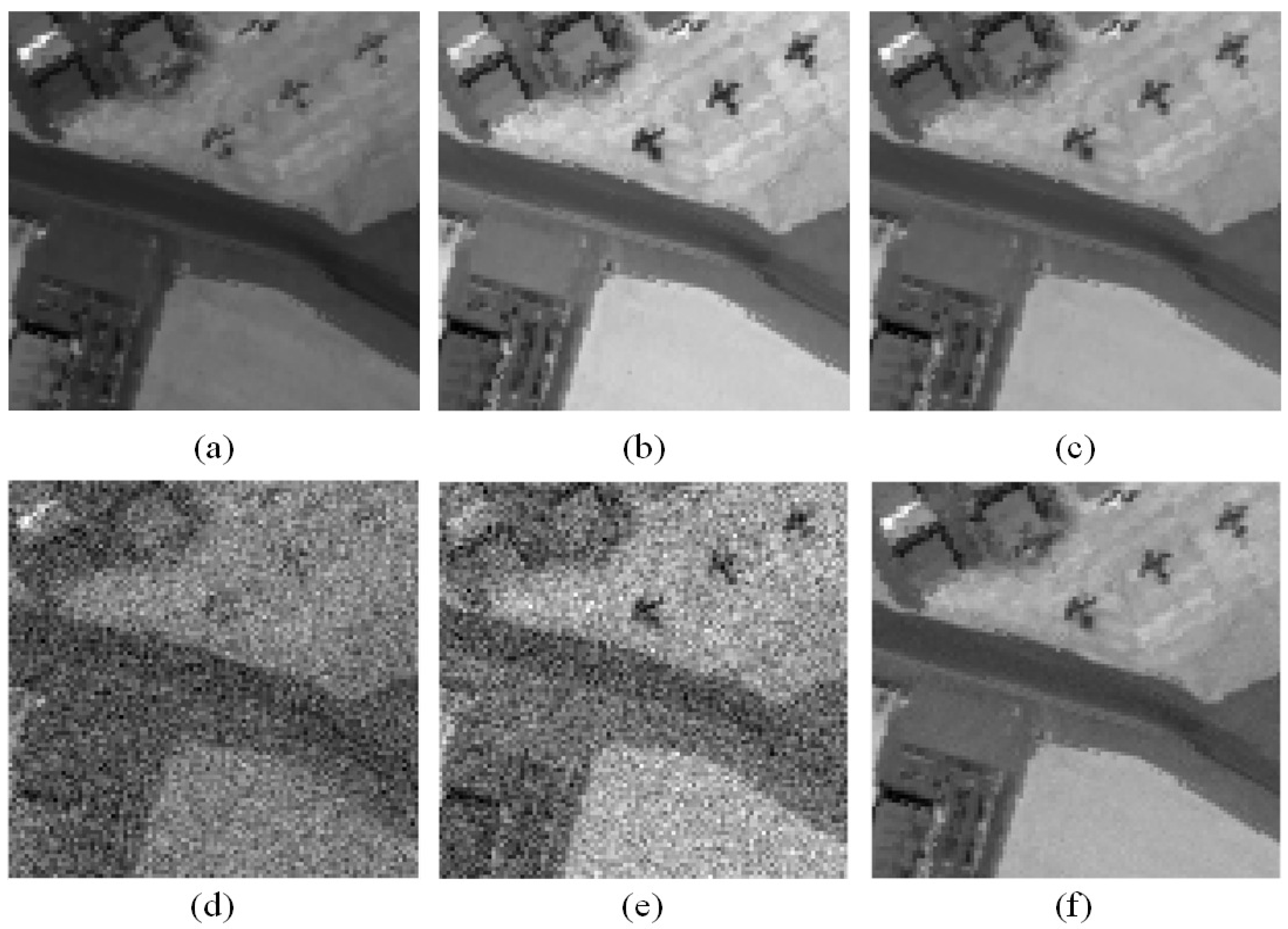
2.2.1. Redundant Spectral Channels

HSI is a 3-dimension (3D) cube that contains a large number of spectral channels. However, some of these channels are unsuitable for detecting anomalies due to their low contrast against the background. As shown in Figure 1, Figure 1a,b are acquired from the AVIRIS dataset. The airplanes in Figure 1a (the 20th band) present lower contrast than in Figure 1b (the 150th band). These redundant channels are counterproductive to target detection, and dimensionality reduction is needed to remove the redundant spectral images. Principal component analysis (PCA) is an unsupervised linear approach where cumulative-variance accumulation is adopted for selecting best characteristics from HSI data [25,26]. To efficiently remove redundant spectral bands, we employ the PCA model in our framework. As shown in Figure 1c, the first principal component map presents a clear contrast of airplanes in comparison with Figure 1a. The PCA model can effectively reduce the next operation processing burden, making it suitable for practical applications. More importantly, the PCA model has strong anti-noise ability (especially the random noise), since most of the random noise centers on the high-rank maps of HSIs [27] and these parts are abandoned in our algorithm. Figure 1d–f depicts the noise HSIs (adding Gaussian noise with $\sigma =0.1$), corresponding to Figure 1a–c, respectively. Figure 1f demonstrates an excellent noise suppression result.

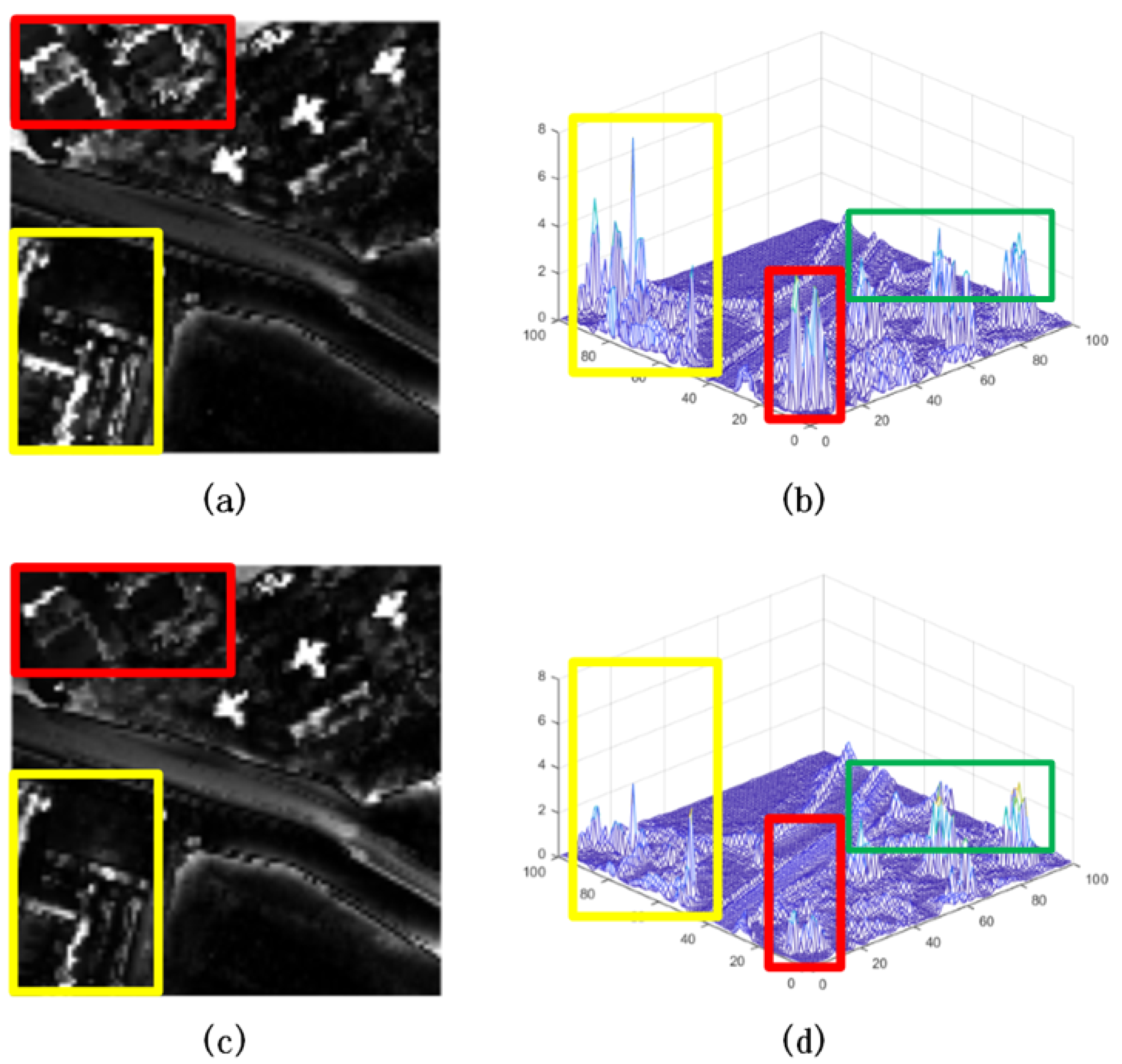
2.2.2. Complicated Backgrounds

As mentioned before, ground features are complex and can cause confusion between a target and similar edge areas, such as buildings, which may be abnormal against the background. To better detect the anomalies, we adopt a fast guided filter [28] for purifying and removing the background, so targets will be distinguishable in the difference maps. As shown in Figure 2a, the three airplanes are distinguishable in the map of the AD result. However, the edges of the background highlighted by red and yellow rectangles in Figure 2 create strong interference in target detection. In this paper, we design an edge-weight operation for a guided filter to extract the edge regions from HSI data, while reducing the edge region in difference maps. As shown in Figure 2c,d, the anomaly values in red and yellow rectangles decrease considerably, demonstrating the effectiveness of this operation. More importantly, the areas highlighted by green rectangles are three airplane objects. The abnormality degrees of airplane are almost the same with and without weighted operation proving that weighted operation has little effect on small areas.

3. Method

Figure 3 presents the workflow of the proposed AD framework in which we incorporate the PCA model to compress HSI data and a weighted guided filter to remove the background. The HSI cube is first decomposed by the PCA model to collect remarkable information. This strategy plays a great role in reducing redundant information and random noise for AD application. Then, the improved guided filter is adopted to purify the background, and corresponding difference maps are calculated to detect the anomaly targets. Finally, an efficient diagonal matrix operation is designed to locate the abnormal targets.

3.1. PCA Model

HSIs contain abundant spectral information, but only a few dimensions are actually important for the analysis. The PCA model adopts orthogonal statistical transformation to identify the correlations amongst HSI bands for mining essential features [26]. It can represent hyperspectral data in a more compact cube without losing too much information. While numerous improved PCA models are available, such as Kernel-PCA [29] and Morphological-PCA [30], we chose linear PCA due to the peculiarities of low complexity which already is an embedded fuction of matlab software.

Suppose that $X\in R^{(L\times M\times N)}$ refers to HSI data, where M, N, and L are the width, height, and spectral channel, respectively. Then, the HSI data X are reshaped into matrix $I\in R^{L\times (M·N)}$ and the mean value of ith band is as follows:

$$I_{mean}\left(i\right)=\frac{1}{M·N}\sum _{j=1}^{M·N}I(i,j).$$

(1)

Then, the mean matrix can be expanded to $I_{\in }{R}^{L\times (M·N)}$ where $I_{mean}(i,j)=I_{mean}\left(i\right),\forall j=1,\dots ,(M·N)$, and the covariance matrix C of I is calculated as follows:

$$C=\frac{1}{M·N-1}\left(I-I_{mean}\right){\left(I-I_{mean}\right)}^T.$$

(2)

The eigenvalues $E=[e_1,\dots ,e_L]$ and eigenvectors $V=[v_1,\dots ,v_L]$ of covariance matrix C are obtained as follows:

$$C=VE{V}^T,$$

(3)

where T represents the transpose operation. Then, the eigenvectors are sorted by decreasing eigenvalues and we select the first b eigenvectors corresponding to the first b eigen to build a new matrix $V_b=[v_1,\dots ,v_b]$. Finally, the original HSI can be projected into a new feature space as:

$$I_{pca}=V_b^T\left(I-I_{mean}\right),$$

(4)

where matrix $I_{pca}\in R^{k\times (M·N)}$ is the result of dimensionality reduction.

3.2. Weighted Guided Filter

The fast guided filter was proposed by He and Sun [31] based on the guided filter [28] and a first-order constraint. Compared with other edge-preserving algorithms, the fast guided filter contains a simple linear transform, making it suitable for practical applicationa. Suppose the guide image, filtering input image, and filtering output image are $I_g$, $I_{pca}$, and $I_{new}$, respectively. The guided filter is driven by a local linear model as follows:

$$I_{new}\left(i\right)=a_k{I}_g\left(i\right)+b_k,\forall i\in w_k,$$

(5)

where i is the index of image pixels, $a_k$ and $b_k$ are the projection parameters, and k is the index of local window w, which has a radius r. By minimizing the reconstruction error between $I_{pca}$ and $I_{new}$, we can acquire $a_k$ and $b_k$ as follows:

$$a_k=\frac{\frac{1}{\left|w\right|}{\sum }_{i\in w_k}{I}_g\left(i\right)I_{pca}\left(i\right)-{\mu }_k{\overline{I}}_{pca}\left(k\right)}{{\sigma }_k^2+\epsilon }$$

(6)

$$b_k={\overline{I}}_{pca}\left(k\right)-a_k{\mu }_k,$$

(7)

where ${\mu }_k$ and ${\sigma }_k$ are the mean and variance of $I_g$ in window k, respectively; and ε is a regularization parameter controlling the degree of smoothness. The parameters r controls the filter window size, bigger window size means more background region will be filtered by the weighted guided filter. The parameters $\epsilon$ determines the smoothness degree, the bigger ε, the deeper the degree of smoothness. The setting of parameters r and ε were discussed in the Evaluation indexes and Parameter Setting subsection. The filtering output is computed by:

$$I_{new}\left(i\right)={\overline{a}}_i{I}_g\left(i\right)+{\overline{b}}_i,$$

(8)

where ${\overline{a}}_i=\frac{1}{|w_i|}{\sum }_{k\in w_i}{a}_k$ and ${\overline{b}}_i=\frac{1}{|w_i|}{\sum }_{k\in w_i}{b}_k$ are the average of a and b, respectively, on window $w_i$ centered at i. To extract the structure of input image, we design an edge-weight G for input image $I_{pca}$ as follows:

$$G\left(k^{\prime }\right)=\frac{1}{\left|w\right|}\left(\sum _{i\in w_{k^{\prime }}}{I}_{pca}^2\left(i\right)-{\left(\sum _{i\in w_{k^{\prime }}}{I}_{pca}\left(i\right)\right)}^2\right),$$

(9)

where $G\left(k^{\prime }\right)$ is computed in window $3\times 3$. We apply a Gaussian function $Ga$ to smooth weight G maps so that local valuess of weight G maps are stable. Gaussian function matrix was created by Gaussian function with a standard variation of 2 using MATLAB. This matrix was inspired by SSIM method [32] to smooth weight G maps. The Gaussian function matrix $Ga$ we used here is as follows:

$$\left(\begin{array}{ccccc}0.0232& 0.0338& 0.0383& 0.0338& 0.0232\\ 0.0338& 0.0492& 0.0558& 0.0492& 0.0338\\ 0.0383& 0.0558& 0.0632& 0.0558& 0.0383\\ 0.0338& 0.0492& 0.0558& 0.0492& 0.0338\\ 0.0232& 0.0338& 0.0383& 0.0338& 0.0232\end{array}\right)$$

(10)

The parameter ε is divided by weight G maps so that $a_k$ increases with weight G. This operation will preserve the main structure of background. The corresponding parameter $a_k$ is updated as follows:

$$a_k=\frac{\frac{1}{\left|w\right|}{\sum }_{i\in w_k}{I}_g\left(i\right)I_{pca}\left(i\right)-{\mu }_k{\overline{I}}_{pca}\left(k\right)}{{\sigma }_k^2+\epsilon /G}.$$

(11)

Diverse guide images exists, such as original spectral channels or the results of PCA. We adopt the results of PCA as the guide image, i.e., $I_g=I_{pca}$, and $a_k$ and $b_k$ are calculated as follows:

$$a_k=\frac{{\sigma }_k^2}{{\sigma }_k^2+\epsilon /G}$$

(12)

$$b_k=(1-a_k){\overline{p}}_k.$$

(13)

It is obvious that the improved filter is an effective edge-preserving filter. Parameter $a_k$ increases in the edge areas to extract the main structure. We adopt the improved guided filter to purify the background, and the difference images $I_{diff}$ are calculated as: $I_{diff}=I_{pca}-I_{new}$. Then, the difference images are employed to detect abnormal targets, since the background is different from the anomalies that are locally continuous in the spatial domain [33].

3.3. Diagonal Matrix Operation

The difference images contain anomaly targets and many methods can be applied to locate these objects. The Mahalanobis distance of RX is one of the common methods used for detecting anomalies. However, the inversion of the covariance matrix for the whole image is complex and computationally intensive. We removed the background, and so did not need a normalization operation or linear projection. Given the convenience of the matrix calculation in MATLAB, we designed a diagonal matrix operation to efficiently collect the energy of each pixel between the channels of the difference images $I_{diff}\in R^{\left(\right(M·N)\times b)}$. The operation is as follows:

$$Y=diag\left(I_{diff}*I_{diff}^T\right),$$

(14)

where $diag$ is the operation that extracts the diagonal element of matrix $I_{diff}*I_{diff}^T$. Formula (14) sums the square values of each pixel in the difference images $I_{diff}$ to determine the energy accumulation for anomalies. Then, the AD result can be acquired, as shown in Figure 2d. To reduce the computation complexity and memory requirement, we employ “for cycle” for all the $M·N$ pixels to accumulate the energy of each channel.

3.4. Evaluation indexes and Parameter Setting

We used the ROC curve and AUC to evaluate the detection accuracy of the considered methods. The ROC values represent the changes in detection performance $P_D$ (probability of detection) with false alarm $P_{FA}$. When a specific threshold $\eta$ is adopted to measure the anomalies, $P_D$ and $P_{FA}$ are as follows:

$$P_D=\frac{N_{TT}}{N_T},P_{FA}=\frac{N_{BT}}{N_B},$$

(15)

where $N_{TT}$ represents the number of true targets labeled as targets, $N_T$ denotes the total number of targets (anomalies), $N_{BT}$ is the number of background pixels labeled as targets, and $N_B$ counts the total number of background pixels. AUC calculates the area under the ROC curve. There are two groups of parameters that need to be adjusted: (1) The number of dimensionality-reduction maps and (2) filter parameters r and ε. These parameters play important roles in AD detection.

3.4.1. The Number of Dimensionality-Reduction Maps

PCA is an unsupervised dimensionality reduction method requiring a preset channel number. To select a suitable number of PCA maps, we tested our model on the first AVIRIS dataset. As shown in Figure 4a, the AUC values increase with the number of dimensionality-reduction maps (with a channel number under five). This demonstrates that increasing the number of maps improves AD performance. The energy of targets concentrates in the front part of principal components. Therefore, the increasing of channel numbers will enhance target energy which can improve the effect of anomaly detection. The target detection is not affected when exceeding five PCA maps. However, the computational complexity of the guilder filter is increased with the number of PCA maps. To reduce the computational time, we chose five PCA maps for our model. Based on lots of experiments, we select first five principal components to detect the abnormal areas and this condition is applied to all HSI images.

3.4.2. Filter Parameters r and ε

Parameter r and ε control the size of the window and the degree of smoothness. To find the optimal r and ε, we tested the AUC values with filter parameters ranging from 1 to 17. Figure 4b presents the visualized result on the first AVIRIS dataset. We found the detection performance is sensitive to the window size r and a better performance can be obtained when r and ε are 11 and 5, respectively. For the AVIRIS-II data set, it contains similar landcover features and targets to the AVIRIS-I data. Then, we use the same parameters for those two datasets.

For the HYDICE dataset, it contains smaller targets comparing with AVIRIS-I and AVIRIS-II dataset, and we achieved a better detection performance when the $r=9$ and $\epsilon =0.2$. As window size r determined how many background regions will be processed by the filter, larger targets seems need larger filter window size to wrap it. Then, for the Pavia Centre dataset, which contains targets with the size larger than the HYDICE dataset but smaller than the AVIRIS-I dataset, we set $r=10$ and $\epsilon =5$ to test the detection performance. For the simulated dataset, it contains pixel and sub-pixel targets with a smaller size than other dataset, then we set a much smaller filter windows size for it with $r=2$ and $\epsilon =3$ to test the detection performance.

4. Experimental Results and Discussion

In this section, we compare our model with state-of-the-art AD methods on four public datasets and one simulated dataset. We compare the performance of the proposed approach with other AD algorithms including RX [9] (hyperspectral toolbox in github) [34], RX on discrete wavelet transform (RX-DWT) [14] (FrFE toolbox in github) [35], RX-Kernel [11] (hyperspectral toolbox in github) [34], robust PCA [15] (FEBPAD toolbox in github) [36], LSMAD [16] (FEBPAD toolbox in github) [36], LRASR [17] (LRASR toolbox in github) [36], FrFE [14] (FrFE toolbox in github) [35], GTVLRR [19] (FEBPAD toolbox in github) [37], and FEBPAD [20] (FEBPAD toolbox in github) [37]. We report the area under the curve (AUC) [38] and receiver operating characteristic (ROC) curve [39] on the different datasets, and present the corresponding detection maps. Moreover, we compare our model with others on Gaussian and impulse noise data to prove the robustness of our model. Finally, we present the testing time of our model.

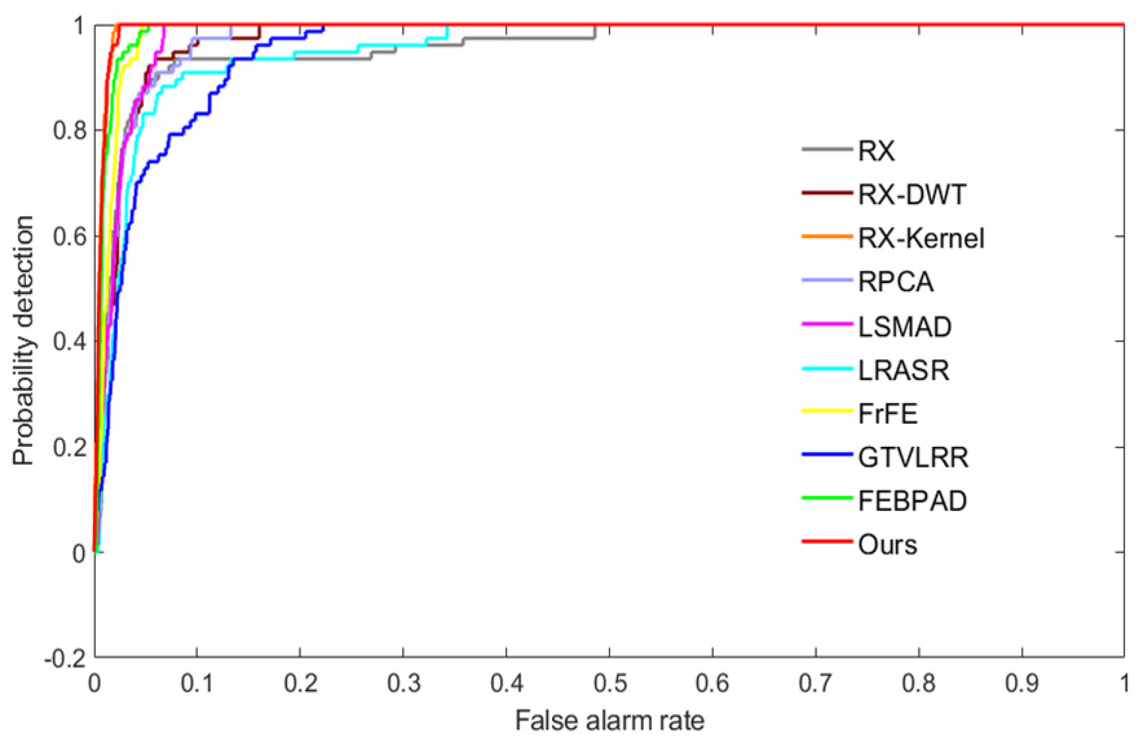
4.1. Detection Performance Analysis

4.1.1. The AVIRIS-I Dataset

We compared our model with the state-of-the-art models on four public datasets. For the AVIRIS-I dataset, Figure 5 presents the detection maps acquired by the various methods. Figure 5a,l are the pseudo-color image and ground truth map, respectively and Figure 5b–k depicts the corresponding detection maps of RX, RK-DWT, RX-Kernel, RPCA, LSMAD, SRALR, FrFE, GTVLRR, FEBPAD, and the proposed method, respectively. It can be seen that the RX-based, RPCA, and FEBPAD methods can correctly detect the anomalies, but their responses values are not strong. The LSMAD, SRALR, and FrFE algorithms achieve a better visual performance than the RX-based ones due to the sparsity constraint for low-probability targets. The GTVLRR model obtains detailed texture background information because of the total variation for high-frequency information. In contrast, our model acquires the best result for the three targets due to purifying and removing the background.

To quantitatively compare our framework with the other state-of-the-art models, the ROC curves with pointwise confidence intervals are exhibited in Figure 6, and the AUC values with upper and lower bounds are reported in

Table 2. AUC values of the proposed method and state-of-the-art methods on three HSI datasets.

Dataset	RX	RX-DWT	RX-Kernel	RPCA	LSMAD
1	0.8865	0.9607	0.9768	0.9782	0.9773
2	0.9578	0.9737	0.9941	0.9739	0.9781
3	0.9700	0.9743	0.9419	0.9852	0.9813
4	0.9538	0.9659	0.9515	0.9570	0.9704
5	0.8107	0.8828	0.8493	0.8105	0.9435
Dataset	LRASR	FrFE	GTVLRR	FEBPAD	Ours
1	0.9704	0.9708	0.9697	0.9886	0.9971
2	0.9550	0.9853	0.9532	0.9899	0.9937
3	0.9665	0.9837	0.9990	0.9917	0.9975
4	0.9592	0.8119	0.9817	0.9354	0.9752
5	0.7697	0.3622	0.9950	0.9725	0.9999

. Figure 6 shows that low-rank AD methods can obtain stable results for three airplanes, whereas RX performs poorly for the first datasets due to the complex spectral channels. Our model performs the best on the AVIRIS-I dataset.

4.1.2. The AVIRIS-II Dataset

Figure 7 shows the visual detection maps of the models compared on the second AVIRIS dataset. Figure 7a,l is the pseudo-color image and ground truth map, respectively; Figure 7b–k is the detection maps of RX, RK-DWT, RX-Kernel, RPCA, LSMAD, SRALR, FrFE, GTVLRR, FEBPAD, and the proposed method, respectively. The RX-Kernel, SRALR, and FrFE models produce better visual effects than the RX and RPCA models. GTVLRR retains abundant texture of background, which will limit the detection performance. Our model acquires the best visual result for the three targets, being the closest to the ground truth amongst the all the compared state-of-the-art methods.

To clearly explain the detection result, we exhibit the ROC curves in Figure 8 and report the AUC values in Table 2. In Figure 8, we can observe that RX, the SRALR, and GTVLRR models obtain the worst results. Our model obtains comparable, but slightly worse, performance on the second AVIRIS dataset to the best-performing RX-Kernel.

4.1.3. The HYDICE Dataset

For illustrative purposes, Figure 9 presents the obtained detection maps of the compared algorithms on the HYDICE dataset. Figure 9a,l is the pseudo-color image and ground truth map, respectively; Figure 9b–k is the detection maps of RX, RK-DWT, RX-Kernel, RPCA, LSMAD, SRALR, FrFE, GTVLRR, FEBPAD, and the proposed method, respectively. From the illustrative presentation of the detection maps, we find that RPCA and our model provide excellent background suppression performance. The result of our model is the closest to the ground truth amongst all the considered state-of-the-art methods.

We exhibit the ROC curve in Figure 10 and list the AUC values in Table 2. As shown in Figure 10, the proposed algorithm achieves outstanding performance compared with the other methods in terms of ROC and AUC values, which demonstrates the effectiveness of the proposed AD model.

4.1.4. The Pavia Centre Dataset

To prove the detection effect of the proposed method, we compared it with other AD algorithms on the Pavia Centre dataset, which has a larger spatial domain. Figure 11a,l present the pseudo-color image and ground truth map, respectively; Figure 11b–k shows the detection results of these models. From the detection maps, the FrFE, GTVLRR, and FEBPAD models have poor background suppression capability. Our model can effectively remove the background and the detection map is similar to the ground truth.

For quantitative comparisons, we present the ROC curve in Figure 12 and report the AUC values in Table 2. In Figure 12, the red curve associated with our method is close to the upper right corner, which demonstrates the effectiveness of the proposed model. The AUC value of our method is 0.9752, only slightly less than that of GTVLRR, at 0.9817. However, our model has lower computational complexity and is robust against noise interference.

4.1.5. The Simulated Dataset

To demonstrate the point target or sub-pixel target detection effect of our method, we tested the AD algorithms on the simulated dataset, which contains different proportions of mixed pixels. Figure 13a,l exhibits the pseudo-color image and ground truth map, respectively; Figure 13b–k presents the corresponding detection results of these algorithms. As can be seen from visual result, RPCA, LSMAD, and GTVLRR models can effectively suppress the background. Nevertheless, their detection effect is poor on sub-pixel targets with a low proportion in the left of the simulated image. Our method is the closest to the ground truth of these state-of-the-art algorithms, proving the effectiveness of our model.

For quantitative comparisons, we present the ROC curve in Figure 14 and report the AUC values in Table 2. In Figure 14, the red curve associated with our method is closest to the upper right corner. Remarkably, our model achieves the best AUC value. All these results indicate that the proposed model can effectively distinguish anomalies from the background.

4.2. Noise Interference

Gaussian noise: Hyperspectral data have been widely applied for target detection. However, one obstacle [40] to HSI applications is that HSIs are often corrupted by Gaussian noise. Gaussian noise limits the application of HSI data and degrades AD performance. AD algorithms need to have an inherent capability to counteract the effects of Gaussian noise interference. To prove the ability of our method to resist the effects of Gaussian noise, we compared our model with the state-of-the-art algorithms under different degrees of Gaussian noise [41].

Table 3. AUC values of the proposed method and methods used for comparison on the AVIRIS-I dataset under different degrees of Gaussian noise.

Noise $\mathit{\sigma }$	RX	RX-DWT	RX-Kernel	RPCA	LSMAD	LRASR	FrFE	GTVLRR	FEBPAD	Proposed
0.00	0.8865	0.9607	0.9768	0.9782	0.9773	0.9704	0.9708	0.9697	0.9886	0.9971
0.10	0.7541	0.8233	0.9767	0.8090	0.8954	0.9311	0.7890	0.9187	0.9424	0.9922
0.22	0.6307	0.6959	0.9156	0.6501	0.8053	0.7056	0.6389	0.5192	0.6522	0.9835
0.31	0.5722	0.6303	0.8043	0.5902	0.7215	0.5946	0.5587	0.5021	0.5019	0.9728
0.40	0.5988	0.6115	0.7936	0.6062	0.6761	0.5522	0.5321	0.5040	0.4920	0.9307
0.52	0.5522	0.5980	0.6836	0.5255	0.5283	0.5547	0.5008	0.4834	0.4325	0.8972
0.61	0.5016	0.5680	0.5680	0.5680	0.5723	0.5039	0.4430	0.4993	0.3385	0.8359
0.84	0.4783	0.5246	0.4811	0.4560	0.4909	0.4633	0.4807	0.5162	0.3909	0.7214
0.94	0.4773	0.4613	0.5121	0.4592	0.5046	0.4335	0.4891	0.5002	0.3822	0.6799
1.10	0.5197	0.5769	0.4681	0.4882	0.4700	0.5024	0.4603	0.5385	0.4249	0.6337
1.35	0.4772	0.5092	0.5334	0.4561	0.4472	0.4822	0.4633	0.5007	0.4519	0.6297
1.50	0.4776	0.4770	0.4779	0.4690	0.4721	0.4619	0.5311	0.5120	0.4715	0.5603

and Figure 15 present the AUC values on the AVIRIS-I dataset under different degrees of Gaussian noise. We can see that the rate at which the detection performance of proposed model decreases is the slowest with increasing Gaussian noise due to the introduction of PCA model. The detection performance of proposed model is much higher than second best model (RX-Kernel) which adopts higher-dimensional space to detect anomalies.

For illustrative purposes, Figure 16 presents the obtained detection maps of the considered algorithms on the AVIRIS-I dataset with Gaussian noise $\sigma =0.1$. Figure 16a,l is the pseudo-color image and ground truth map, respectively; Figure 16b–k is the detection maps of RX, RK-DWT, RX-Kernel, RPCA, LSMAD, SRALR, FrFE, GTVLRR, FEBPAD, and the proposed method, respectively. The original image and most detection maps are severely contaminated by Gaussian noise. RX-Kernel and our model achieve better detection results than the other state-of-the-art methods and our model is the closest to the ground truth.

Impulse noise: To prove the superior ability of our method to resist impulse noise, we compared our model with the state-of-the-art algorithms under different degrees of impulse noise. Figure 17 exhibits the AUC values on the AVIRIS-I dataset under different degrees of impulse noise. We can see that the rate at which the detection performance of the proposed model decreases is the slowest with increasing impulse noise. The detection performance of the proposed model is much higher than that of the next-best model (RX-Kernel). Figure 18 shows the detection maps on the AVIRIS-I dataset with 0.2% impulse noise. Figure 18a,l is the pseudo-color image and ground truth map, respectively; Figure 18b–k is the detection maps of RX, RK-DWT, RX-Kernel, RPCA, LSMAD, SRALR, FrFE, GTVLRR, FEBPAD, and the proposed method, respectively. The original image and most detection maps are severely contaminated by impulse noise. The impulse noise is similar to anomalies and will seriously interfere with AD performance, especially for the low-rank models using a sparsity constraint. RX-Kernel and our model achieve better detection results than the other state-of-the-art methods and our model is the closest to the ground truth.

Real noise: To demonstrate the anti-noise property, we conducted an additional experiment on the AVIRIS-I dataset without removing the noise bands. The number of spectral band is 224 and partial bands are contaminated by real noise. The ROC curve and AUC values are presented in Figure 19 and

Table 4. AUC values of the proposed method and methods used for comparison on the first AVIRIS dataset without removing the noise bands.

Dataset	RX	RX-DWT	RX-Kernel	RPCA	LSMAD
224 bands	0.8454	0.8579	0.9798	0.9711	0.9795
Dataset	LRASR	FrFE	GTVLRR	FEBPAD	Ours
224 bands	0.9764	0.9566	0.9675	0.9782	0.9964

. It is obvious that the proposed method always offers the best detection performance even when the probability of false alarm is extremely low. Our model achieves the best performance in terms of AUC values with a 2-point lead over the second place. The AUC value of our model declines by only 0.07% under the interference of noised bands which demonstrates the robustness of our model.

4.3. Time Cost

All the experiments in this study were implement in MATLAB on a Windows 10 operation system and conducted on an Intel Core I7-8700 CPU 3.20GHz desktop with 16 GB memory. From

Table 5. The computation costs of different AD methods on the three datasets (in seconds).

Dataset	RX	RX-DWT	RX-Kernel	RPCA	LSMAD
1	0.0988	4.5790	61.3003	9.0523	8.3447
2	0.0932	4.6329	77.7485	14.2317	8.4044
3	0.0746	3.3241	37.5660	6.8391	5.1366
4	0.1204	6.1317	3104.4629	81.842	14.6488
5	0.1822	7.3317	440.6284	19.8474	18.7047
Dataset	LRASR	FrFE	GTVLRR	FEBPAD	Ours
1	10.9892	15.8958	89.7813	2.3781	0.3772
2	10.8809	16.7092	94.6053	2.3582	0.3711
3	8.3371	10.9782	74.3376	1.6061	0.2957
4	19.9892	13.4504	159.1784	6.3693	1.2113
5	21.686	22.3962	144.936	5.9663	0.9265

, we can see that our model is faster than the other state-of-the-art methods except for the RX model, which adopts linear projection to extract the anomalies. This proves the practical value of our model for HSI application. The main reasons for the efficient detection ability of our model are twofold: (1) A PCA model is adopted to reduce the spectral channels of the subsequent computations; (2) an efficient diagonal matrix operation is used to quickly locate the anomalies.

4.4. Detection Performance Discussion

Based on the previous experimental results, our algorithm has shown great potential in hyperspectral anomaly detection. Experiments result on AVIRIS-I and AVIRIS-II datasets illustrates that, our method achieved the highest AUC values comparing with other methods under the same parameters ($r=11$, $\epsilon =5$) as those two datasets contain similar land features and targets. Experiments result on simulated data set demonstrate that our method is suitable and effective for sub-pixel targets and shown better performance under smaller filter window size ($r=2$, $\epsilon =3$). Those three datasets are collected by AVIRIS sensors with different land covers and the test results seems stable with the smoothness degree but sensitive to filter window size. For the dataset collected by other sensors (HYDICE and ROSIS), our method achieves satisfactory results by adjusting the parameters.

The main differences between the datasets we used (collected by AVIRIS, HYDICE and ROSIS sensors with different spatial resolution) are the size of anomaly targets and landcover features they contained, bigger targets and complex landcovers need larger filter window size and smoothness degree to purify the background. Even though there are no prior spectral information of the targets but what we want to detect can be used as a guide for parameter settings. Then, we use a smaller smoothness degree and window size for small targets under HYDICE and Pavia data set to test the detection performance and achieve satisfactory results. In other words, the parameters are sensitives to the HSI data source and targets size, they are better to be changed with the variation of the data source and observation scene. Based on our tests, smoothness degree parameter ε can be selected from 3–5 for AVIRIS and ROSIS sensors. For the data collected from HYDICE sensors with pixel or sub-pixel targets, ε can be selected from 0.1–0.3. The window size parameter r can be set as twice bigger than the targets you suspected contains in the hyperspectral images.

5. Conclusions

In this work, we constructed an efficient and robust anomaly detection framework. Extensive experiments were conducted on four public datasets and one simulated dataset, demonstrating that our proposed scheme outperforms the state-of-the-art methods in terms of detection time and accuracy. Furthermore, the proposed approach has shown better robustness under severe Gaussian noise pollution.

As for the possible shortcomings of the proposed work, the parameters in weighted guided filter processing should be more adaptive to the HSI source and targets. How to select parameters automatically for different data sources to detect targets with different sizes will be a focus in our future work. A multi-scale filter structure which contains filters with different filter window sizes seems to be a suitable way to avoid the parameter setting process and we will try to use this technique to improve our model in the future. In addition, due to the availability of HSI public data sets, there are three kinds of sensor data conducted, and other sensor images could be further tested or verified in future work to discover the relationship between parameters and sensors and establish a model to realize the adaptive parameter adjustment.

Moreover, we employ PCA to reduce the spectral channel, and we are aware that in some advanced works, feature selection has been realized in optics target detection tasks and time series processing tasks. We consider that a similar approach should also be feasible for AD of HSIs. In our future work, we will continue to improve our approach by adopting efficient characteristic spectral band selection models.

References

1. Ghamisi, P.; Plaza, J.; Chen, Y.; Li, J.; Plaza, A. Advanced Spectral Classifiers for Hyperspectral Images: A Review. IEEE Geosci. Remote Sens. Mag. 2017, 5, 8–32. [Google Scholar] [CrossRef] [Green Version]
2. Jafarzadeh, H.; Hasanlou, M. An Unsupervised Binary and Multiple Change Detection Approach for Hyperspectral Imagery Based on Spectral Unmixing. IEEE J. Sel. Top. Appl. Earth Observ. Remote Sens. 2019, 12, 4888–4906. [Google Scholar] [CrossRef]
3. Li, Z.; Zhao, B.; Wang, W. An Efficient Spectral Feature Extraction Framework for Hyperspectral Images. Remote Sens. 2020, 12, 3967. [Google Scholar] [CrossRef]
4. Tan, K.; Hou, Z.; Ma, D.; Chen, Y.; Du, Q. Anomaly Detection in Hyperspectral Imagery Based on Low-Rank Representation Incorporating a Spatial Constraint. Remote Sens. 2019, 11, 1578. [Google Scholar] [CrossRef] [Green Version]
5. Shimoni, M.; Haelterman, R.; Perneel, C. Hypersectral Imaging for Military and Security Applications: Combining Myriad Processing and Sensing Techniques. IEEE Geosci. Remote Sens. Mag. 2019, 7, 101–117. [Google Scholar] [CrossRef]
6. Karami, A.; Heylen, R.; Scheunders, P. Hyperspectral image noise reduction and its effect on spectral unmixing. In Proceedings of the 2014 6th Workshop on Hyperspectral Image and Signal Processing: Evolution in Remote Sensing (WHISPERS), Lausanne, Switzerland, 24–27 June 2014; pp. 1–4. [Google Scholar]
7. Zhang, C.; Zhou, L.; Zhao, Y.; Zhu, S.; Liu, F.; He, Y. Noise reduction in the spectral domain of hyperspectral images using denoising autoencoder methods. Chemom. Intell. Lab. Systems. 2020, 203, 104063. [Google Scholar] [CrossRef]
8. Awad, M. Forest mapping: A comparison between hyperspectral and multispectral images and technologies. J. For. Res. 2018, 29, 1395–1405. [Google Scholar] [CrossRef]
9. Reed, I.S.; Yu, X. Adaptive Multiple-Band CFAR Detection of an Optical Pattern with Unknown Spectral Distribution. IEEE Trans. Acoust. Speech Signal Process. 1990, 38, 1760–1770. [Google Scholar] [CrossRef]
10. Chang, C.I.; Chiang, S.S. Anomaly Detection and Classification for Hyperspectral Imagery. IEEE Trans. Geosci. Remote Sens. 2002, 40, 1314–1325. [Google Scholar] [CrossRef] [Green Version]
11. Kwon, H.; Nasrabadi, N.M. Kernel RX-Algorithm: A Nonlinear Anomaly Detector for Hyper-Spectral Imagery. IEEE Trans. Geosci. Remote Sens. 2005, 43, 388–397. [Google Scholar] [CrossRef]
12. Matteoli, S.; Veracini, T.; Diani, M.; Corsini, G. A Locally Adaptive Background Density Estimator: An Evolution for RX-based Anomaly Detectors. IEEE Geosci. Remote Sens. Lett. 2014, 11, 323–327. [Google Scholar] [CrossRef]
13. Wang, W.; Zhao, B.; Feng, F.; Nan, J.; Li, C. Hierarchical Sub-Pixel Anomaly Detection Framework for Hyperspectral Imagery. Sensors 2018, 18, 3662. [Google Scholar] [CrossRef] [Green Version]
14. Tao, R.; Zhao, X.; Li, W.; Li, H.; Du, Q. Hyperspectral Anomaly Detection by Fractional Fourier Entropy. IEEE J. Sel. Top. Appl. Earth Observ. Remote Sens. 2019, 12, 4920–4929. [Google Scholar] [CrossRef]
15. Chen, S.-Y.; Yang, S.; Kalpakis, K.; Chang, C.-I. Low-rank Decomposition-based Anomaly Detection. Algorithms and Technologies for Multispectral, Hyperspectral, and Ultraspectral Imagery XIX, Baltimore, MD, USA, 18 May 2013; 8743, p. 87430N. [Google Scholar]
16. Zhang, Y.; Du, B.; Zhang, L.; Wang, S. A Low-Rank and Sparse Matrix Decomposition-Based Mahalanobis Distance Method for Hyperspectral Anomaly Detection. IEEE Trans. Geosci. Remote Sens. 2016, 54, 1376–1389. [Google Scholar] [CrossRef]
17. Xu, Y.; Wu, Z.; Li, J.; Plaza, A. Anomaly Detection in Hyperspectral Images Based on Low-Rank and Sparse Representation. IEEE Trans. Geosci. Remote Sens. 2016, 54, 1990–2000. [Google Scholar] [CrossRef]
18. Zhang, L.; Cheng, B.; Deng, Y. A Tensor-based Adaptive Subspace Detector for Hyperspectral Anomaly Detection. Int. J. Remote Sens. 2018, 39, 2366–2382. [Google Scholar] [CrossRef]
19. Cheng, T.; Wang, B. Graph and Total Variation Regularized Low-rank Representation for Hyperspectral Anomaly Detection. IEEE Trans. Geosci. Remote Sens. 2019, 58, 391–406. [Google Scholar] [CrossRef]
20. Ma, Y.; Fan, G.; Jin, Q. Hyperspectral Anomaly Detection via Integration of Feature Extraction and Background Purification. IEEE Geosci. Remote Sens. Lett. 2020. Early access. [Google Scholar] [CrossRef]
21. Huyan, N.; Zhang, X.; Zhou, H.; Jiao, L. Hyperspectral Anomaly Detection via Background and Potential Anomaly Dictionaries Construction. IEEE Trans. Geosci. Remote Sens. 2019, 57, 2263–2276. [Google Scholar] [CrossRef] [Green Version]
22. Xiang, P.; Song, J.; Li, H.; Gu, L. Zhou, H. Hyperspectral Anomaly Detection with Harmonic Analysis and Low-Rank Decomposition. Remote Sens. 2019, 11, 3028. [Google Scholar] [CrossRef] [Green Version]
23. Liu, J.; Hou, Z.; Li, W.; Tao, R.; Orlando, D.; Li, H. Multipixel Anomaly Detection With Unknown Patterns for Hyperspectral Imagery. IEEE Trans. Neural Netw. Learn. Syst. 2021. Early access. [Google Scholar]
24. Zhao, C.; Wang, X.; Zhao, G. Detection of hyperspectral anomalies using density estimation and collaborative representation. Remote Sens. Lett. 2017, 8, 1025–1033. [Google Scholar] [CrossRef]
25. Machidon, A.L.; Del Frate, F.; Picchiani, M.; Machidon, O.M.; Ogrutan, P.L. Geometrical Approximated Principal Component Analysis for Hyperspectral Image Analysis. Remote Sens. 2020, 12, 1698. [Google Scholar] [CrossRef]
26. Uddin, M.P.; Mamun, M.A.; Afjal, M.I.; Hossain, M.A. Information-theoretic Feature Selection with Segmentation-based Folded Principal Component Analysis (PCA) for Hyperspectral Image Classification. Int. J. Remote Sens. 2021, 42, 286–321. [Google Scholar] [CrossRef]
27. Stephan, K.; Hibbitts, C.A.; Hoffmann, H.; Jaumann, R. Reduction of Instrument-dependent Noise in Hyperspectral Image Data using the Principal Component Analysis: Applications to Galileo NIMS Data. Planet. Space Sci. 2008, 56, 406–419. [Google Scholar] [CrossRef]
28. He, K.; Sun, J. Fast Guided Filter. arXiv 2015, arXiv:1505.00996. [Google Scholar]
29. Fauvel, M.; Chanussot, J.; Benediktsson, J.A. Kernel Principal Component Analysis for Feature Reduction in Hyperspectral Image Analysis. In Proceedings of the 7th Nordic Signal Processing Symposium—NORSIG 2006, Reykjavik, Iceland, 7–9 June 2006. [Google Scholar]
30. Franchi, G.; Angulo, J. Morphological Principal Component Analysis for Hyperspectral Image Analysis. Int. J. Geo-Inf. 2016, 5, 83. [Google Scholar] [CrossRef] [Green Version]
31. He, K.; Sun, J.; Tang, X. Guided Image Filtering. IEEE Trans. Pattern Anal. Mach. Intell. 2013, 6, 1397–1409. [Google Scholar] [CrossRef]
32. Wang, Z.; Bovik, A.C.; Sheikh, H.R.; Simoncelli, E.P. Image quality assessment: From error visibility to structural similarity. IEEE Trans Image Process. 2008, 13, 600–612. [Google Scholar] [CrossRef] [Green Version]
33. Shi, C.; Pun, C.M. Superpixel-based 3D Deep Neural Networks for Hyperspectral Image Classification. Pattern Recogn. 2017, 74, 600–616. [Google Scholar] [CrossRef]
34. Hyperspectral Github Toolboxes. Available online: https://github.com/davidkun/HyperSpectralToolbox (accessed on 1 March 2018).
35. FrFE Github Toolboxes. Available online: https://github.com/xudongzhao461 (accessed on 17 September 2021.).
36. LRASR Github Toolboxes. Available online: https://github.com/axiqia (accessed on 17 September 2021.).
37. FEBPAD Github Toolboxes. Available online: https://github.com/l7170 (accessed on 17 September 2021.).
38. Ma, D.; Yuan, Y.; Wang, Q. Hyperspectral Anomaly Detection via Discriminative Feature Learning with Multiple-Dictionary Sparse Representation. Remote Sens. 2018, 10, 745. [Google Scholar] [CrossRef] [Green Version]
39. Chang, C. Multiparameter Receiver Operating Characteristic Analysis for Signal Detection and Classification. IEEE Sens. J. 2010, 10, 423–442. [Google Scholar] [CrossRef]
40. Du, B.; Huang, Z.; Wang, N.; Zhang, Y.; Jia, X. Joint weighted nuclear norm and total variation regularization for hyperspectral image denoising. Int. J. Remote Sens. 2018, 39, 334–355. [Google Scholar] [CrossRef]
41. Acito, N.; Diani, M.; Corsini, G. Signal-Dependent Noise Modeling and Model Parameter Estimation in Hyperspectral Images. IEEE Trans. Geosci. Remote Sens. 2011, 49, 2957–2971. [Google Scholar] [CrossRef]
Figure 1. Visual comparison of different spectral channels in experimental dataset: (a) The 20th channel of AVIRIS-I; (b) the 150th channel of AVIRIS-I; (c) the first principal component map of AVIRIS-I; (d) the corresponding Gaussian noise image of (a); (e) the corresponding Gaussian noise image of (b); (f) the corresponding Gaussian noise image of (c).
Remotesensing 13 04247 g001
Figure 2. Visual comparison for proposed AD algorithm under complicated background: (a) The AD result map of our model with guided filter; (b) 3D map corresponding to (a); (c) the AD result map of our model with weighted guided filter; (d) 3D map corresponding to (c).
Remotesensing 13 04247 g002
Figure 3. The workflow of the proposed anomaly detection framework.
Remotesensing 13 04247 g003
Figure 4. Examples of AUC values under different parameters of our framework: (a) AUC values on the first datasets corresponding to different numbers of dimensionality-reduction maps; (b) AUC values under different filter parameter r and ε .
Remotesensing 13 04247 g004
Figure 5. Detection results on the AVIRIS-I dataset: (a) Pseudo-color image; (b) RX; (c) RX-DWT; (d) RX-Kernel; (e) RPCA; (f) LSMAD; (g) LRASR; (h) FrFE; (i) GTVLRR; (j) FEBPAD; (k) ours; (l) ground truth.
Remotesensing 13 04247 g005
Figure 6. ROC curves of anomaly detectors on the AVIRIS-I dataset.
Remotesensing 13 04247 g006
Figure 7. Detection results on the AVIRIS-II dataset: (a) Pseudo-color image; (b) RX; (c) RX-DWT; (d) RX-Kernel; (e) RPCA; (f) LSMAD; (g) LRASR; (h) FrFE; (i) GTVLRR; (j) FEBPAD; (k) ours; (l) ground truth.
Remotesensing 13 04247 g007
Figure 8. ROC curves of anomaly detectors on the AVIRIS-II dataset.
Remotesensing 13 04247 g008
Figure 9. Detection results on the HYDICE dataset: (a) Pseudo-color image; (b) RX; (c) RX-DWT; (d) RX-Kernel; (e) RPCA; (f) LSMAD; (g) LRASR; (h) FrFE; (i) GTVLRR; (j) FEBPAD; (k) proposed method; (l) ground truth.
Remotesensing 13 04247 g009
Figure 10. ROC curves of anomaly detectors on the HYDICE dataset.
Remotesensing 13 04247 g010
Figure 11. Detection results on the Pavia Centre dataset: (a) Pseudo-color image; (b) RX; (c) RX-DWT; (d) RX-Kernel; (e) RPCA; (f) LSMAD; (g) LRASR; (h) FrFE; (i) GTVLRR; (j) FEBPAD; (k) proposed method; (l) ground truth.
Remotesensing 13 04247 g011
Figure 12. ROC curves of anomaly detectors on the Pavia Centre dataset.
Remotesensing 13 04247 g012
Figure 13. Detection results on the simulated dataset: (a) Pseudo-color image; (b) RX; (c) RX-DWT; (d) RX-Kernel; (e) RPCA; (f) LSMAD; (g) LRASR; (h) FrFE; (i) GTVLRR; (j) FEBPAD; (k) proposed method; (l) ground truth.
Remotesensing 13 04247 g013
Figure 14. ROC curves of anomaly detectors on the simulated dataset.
Remotesensing 13 04247 g014
Figure 15. The AUC results on the AVIRIS-I dataset with the interference of different degrees of Gaussian noise.
Remotesensing 13 04247 g015
Figure 16. Detection results for the AVIRIS-I dataset with Gaussian noise ( σ = 0.1 ): (a) Pseudo-color image; (b) RX; (c) RX-DWT; (d) RX-Kernel; (e) RPCA; (f) LSMAD; (g) LRASR; (h) FrFE; (i) GTVLRR; (j) FEBPAD; (k) proposed method; (l) ground truth.
Remotesensing 13 04247 g016
Figure 17. The AUC results on the AVIRIS-I dataset with different degrees of interference of impulse noise.
Remotesensing 13 04247 g017
Figure 18. Detection results on the AVIRIS-I dataset with impulse noise (proportion): (a) Pseudo-color image; (b) RX; (c) RX-DWT; (d) RX-Kernel; (e) RPCA; (f) LSMAD; (g) LRASR; (h) FrFE; (i) GTVLRR; (j) FEBPAD; (k) proposed method; (l) ground truth.
Remotesensing 13 04247 g018
Figure 19. ROC curves of anomaly detectors on the first AVIRIS dataset without removing the noise bands.
Remotesensing 13 04247 g019