Improving Ship Detection in Clutter-Edge and Multi-Target Scenarios for High-Frequency Radar

Abstract

As one of the main sensors for continuous maritime measurements of sea state parameters, high-frequency surface wave radar (HFSWR) also plays an important role in ship detection and tracking. Compact HFSWR often suffers from missing targets, especially when the target appears near the Doppler region with heavy sea clutter or near another target in a multi-target scenario. To address this problem, an automatic ship detection method based on time–frequency (TF) analysis is presented in this paper. The TF target ridge areas are extracted in the TF image via the eigenvalues of the Hessian matrix, image edge detection, and local maximum search. Then, whether ship signals exist in the TF ridges or not is decided by a decision threshold that is calculated by fitting the probability distribution function (PDF) of sea clutter in the TF domain. The proposed TF method can separate TF ridges of similar Doppler frequency and performs constant false alarm rate (CFAR) detection for TF targets, which facilitates detecting these targets that are masked by sea clutter and other large targets. Experimental results show that the number of detected ships that match with the automatic identification system (AIS) records is four times more than that obtained by the conventional constant false alarm rate (CFAR) detectors and 1.3 times more than that by the state-of-the-art TF method in consideration of approximately the same number of detected targets.

1. Introduction

High-frequency surface wave radar (HFSWR) has the advantages of long detection range, real-time, and continuous operation in all weathers compared with microwave radar [1,2], and has been used in most coastal countries for sustained observations of the ocean surface. Thus far, there are more than 400 HF radar stations around the world for ocean observations [3,4]. By processing the echo data, HFSWRs are used to serve various societal applications such as ocean current and wave monitoring [5], oil spill pollution trajectory forecasting [6], and tsunami warning [7,8], and so on. At the same time, it also plays an important role in ship detection for monitoring the 200-nautical-mile exclusive economic zone. It should be noted that the maximum radar detection range depends on its frequency, bandwidth, and power. With a typical bandwidth of 100 kHz, an operating frequency of 8 MHz, and 30 watts of transmitting power, the WEllen RAdar (WERA) achieves ship detection ranges up to 200 km [9]. With a frequency of 4.55 MHz, a bandwidth of 25 kHz, and an average radiated power of 40 watts, a long-range SeaSonde high-frequency radar can “see” ships to a range of approximately 120 km [10]. According to the antenna type, HFSWR can be classified into two main families [11]. One class is the phased array system. An example of a phased array system is the WERA with a linear receiving antenna array developed by the University of Hamburg [12,13]. WERA was designed to allow for a wide range of working frequencies, spatial resolutions, and antenna configurations. In addition to measuring ocean currents and wave mapping, WERA can also be used for ship target detection and tracking [14,15]. The other class is the crossed-loop/monopole (CLM) antenna system [3]. These radar systems mostly consist of the SeaSonde radar system developed by Coastal Ocean Dynamics Applications Radar (CODAR) Ocean Sensors, Ltd. [16,17]. SeaSonde radars are also used to detect and track ships entering and leaving ports, which achieves multi-use of HF radar [18,19]. Now, real-time vessel detections for the approaches to New York Harbor and the Delaware Bay are provided by SeaSonde radar systems. These detections are supplied to the Naval Research Lab’s (NRL) Open Mongoose data fusion engine where they are turned into vessel tracks using a combination of data from different sensors [20]. Another example is the Ocean State Monitoring and Analyzing Radar (OSMAR) developed by Wuhan University, which is available in both a phased array [21] and compact CLM system [22]. The advantage of a compact CLM radar system is that it can save valuable coastal resources and facilitate installation and maintenance, but its small antenna aperture also means a low spatial gain, which makes the target echoes become more easily submerged by the sea clutter. Meanwhile, the CLM antenna may be distorted due to the surrounding obstacles within a distance of 1–2 wavelengths from the antenna [23]. The surrounding objects may introduce an error of up to 10°–15° to the estimation of the direction of arrival (DOA) [23]. Therefore, for the compact HF radar systems deployed to detect ship targets, some cooperative or non-cooperative signal sources are usually used to calibrate the measured CLM antenna pattern [24,25]. As we know, the ship detection threshold depends on the target radar cross section (RCS). In the HF band, the ship RCS fluctuates within a confined range with radar wavelength [26,27]. Emery et al. [28] found that the ships’ radial velocities and spectral amplitudes can vary significantly as they move within the radar coverage area, and that larger ships are likely to provide stronger backscatter. Small ships tend to have lower RCS since the height of a ship has an important significance on the ship’s RCS [29]. Echoes from small ships are often masked by those from other large ships. Therefore, HFSWR ship detection is a challenging problem.

According to the Bragg scattering mechanism, the first-order echoes appear as two strong spectral peaks symmetrically located on both sides of the zero Doppler frequency, while the surrounding second-order spectral components are lower than their first-order counterparts [30,31]. When the radial velocities of the target and the Bragg wave are approximately the same, the target echo usually falls into the Bragg region so that target masking occurs. In addition, when multiple targets of different sizes at the same distance and direction from the radar have similar radial velocities, the Doppler spectral peaks of large targets tend to mask those of small targets, which can also cause the missed detection of small targets. The detection of small ships is more challenging, and it depends on many factors such as radar frequency, integration time, target cross section, and sea state conditions. The clutter level can be reduced by lowering the radar operating frequency [32,33]. A higher bandwidth and antenna directivity are recommended to reduce the clutter area. A different length of echo data will result in a different signal-to-noise ratio (SNR) of the target and the corresponding detection threshold is also different. Roarty et al. [34] analyzed the relationship between detection threshold and data length, and they found that a coherent integration time (CIT) of 1–2 min had the highest detection probability. Compared with large targets, small targets with a low RCS are more difficult to be detected. The constant false alarm rate (CFAR) algorithm [35,36] has been widely used for radar target detection. For the case of a homogeneous environment, a cell average CFAR (CA-CFAR) [37] is optimal for target detection. However, a homogeneous sea environment is rarely seen in reality. To address the non-homogeneous environments, the smallest of CFAR (SO-CFAR) [38] and the greatest of CFAR (GO-CFAR) [39] were proposed, but the performance of these two detectors drops significantly for targets in the clutter-edge and multi-target scenario, respectively. The ordered statistics CFAR (OS-CFAR) [40] and its variants such as automatic censored mean level CFAR (ACMLD-CFAR) [41], generalized OS-CFAR (GOS-CFAR) [42], and so on were developed, and this type of CFAR processor exhibits a good performance in multi-target and clutter transition situations. The limitation of these methods is that they make assumptions about the nature or composition of the background, but once the assumptions are not valid, as in a real fluctuating environment, their performance drops dramatically. The trimmed-mean CFAR [43] and the variably trimmed-mean CFAR [44] are other types of CFAR detectors, which have a robust performance in a non-homogeneous environment but suffer performance losses in a homogeneous case. In addition, it is difficult to apply a single CFAR detector to work satisfactorily in both homogeneous and non-homogeneous environments, which may occur alternately in practice. To address this problem, composite CFAR detectors were developed for accommodating a variety of environments. For example, the adaptive order statistic (AOS) CFAR [45] and the selection and estimation (SE) test processor [46], and variability index CFAR (VI-CFAR) [47] have the ability to select the appropriate CFAR detector for the current operational environment. The VI-CFAR detector consists of three CFAR detectors: CA-CFAR, GO-CFAR, and SO-CFAR. It selects the most appropriate of these by utilizing the variability index (VI) and mean ratio (MR) statistics. However, the performance of VI-CFAR degrades severely if there are interfering targets distributed on either side of the test cell. Recently, for the scenario with multi-target and targets at the clutter edge, several new CFAR detectors such as cell under test inclusive CFAR [48], first-order difference CFAR (FOD-CFAR) [49], and second-order difference CFAR (SOD-CFAR) [50,51] have been developed. When the statistical distribution characteristics of the clutter do not satisfy the hypothesized distribution, the above CFAR detectors may fail. For SOD-CFAR, the number of interfering targets is estimated based on the minimum of the second-order difference of the ordered samples in the reference window. By using the Shapiro–Wilk (S–W) test [52,53] method, SOD-CFAR implements the uniformity test on the remaining samples after removing interfering targets. However, the S–W test assumes a Gaussian distribution, and it is not suitable for cases with a uniform distribution [54]. In other words, when the distribution characteristic of the clutter located in reference units is not Gaussian, the SOD-CFAR detector may not work. In practical application, the target number and distribution property of reference units are often unknown. Therefore, the decision threshold of the cell under test (CUT) could be easily raised by interference, clutter, and other larger ship targets located in the reference units. As a result, these CFAR detectors generally have a poor detection performance when the target appears at the Bragg peaks’ edge or for cases with multiple targets. To address this problem, the time–frequency constant false alarm rate (TF-CFAR) method is proposed, which can directly extract target ridges and will not be significantly affected by sea clutter and other ship’s signals.

TF representation [55,56,57,58] provides an effective way to analyze multi-component signals and has been applied in radar target detection [59,60,61]. Panagopoulos and Soraghan [62] presented a method for weak target detection by X-band radar using a set of three signal processing techniques (i.e., signal averaging, time–frequency representation, and morphological filtering) to suppress unwanted sea clutter radar echo. However, sea echoes of an X-band radar are quite different from those of an HF radar in terms of time–frequency characteristics [59,63], which limits the application of the method in [62] to only X-band radar. Moreover, it may be inaccurate if the target detection in the TF plane is only based on the duration of TF ridges because such a duration is sometimes shorter than that of sea clutter and interference. For targets at the HFSWR clutter edge, Stankovic et al. proposed a decomposition method based on S transform [64] to separate a target signal from heavy sea clutter. When the target signal approaches the first-order sea clutter in the TF plane, it is very difficult to distinguish the target and clutter decomposition components [65], thus, the S method will fail. To overcome the above disadvantages, Zuo et al. [66] proposed a method based on TF iteration decomposition to detect slow-moving weak targets in sea clutter. Two criteria, i.e., signal duration and time–frequency concentration, are applied to determine the presence of weak target signal components, but they may also be easily affected by sea clutter and interference. In addition, the number of iterations needs to be adjusted manually to obtain the best detection performance for weak targets. Besides the above methods, the combination of TF representation and image segmentation has also been studied and applied in HF radar target detection. Li et al. used discrete wavelet transform to reconstruct ship target signals from the range-Doppler (RD) image contaminated by sea clutter [67]. After the removal of sea clutter and interference, the Ostu algorithm [68] is used for the adaptive segmentation of the RD grayscale images and identification of ship targets. Likewise, the detection threshold also needs to be adjusted adaptively according to clutter intensity, and weak target components may be easily mistaken as background noise. Cai et al. used synchro-extracting transform (SET) to represent radar signals and the Ostu algorithm to extract the TF ridges of ships [69]. Although their method detected weak ship signals successfully, its disadvantages remain the same as [68]. For HFSWR, Yang et al. [70] proposed a TF domain binary integration method to improve the detection of weak target signals, and they reported that the combination of CFAR and TF-CFAR can lead to a further improvement. Although the time–frequency binary integration CFAR (TF-BI-CFAR) in [70] improves the performance of weak targets’ detection, the method still suffers from the masking problem due to strong clutter and large targets, so that the detection performance in the scenarios of multi-target and clutter edge is poor. Later, Yang et al. [71] found that the log-normal distribution was optimal to model sea clutter in the TF domain, and with this model they achieved a better performance for weak and non-stationary target detection than other conventional CFAR detectors.

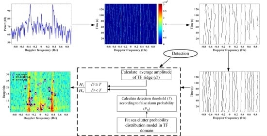
The above target detection methods involving the TF domain analysis mainly focus on signal representations or weak signal detection, and have not given enough consideration to the case of multi-target and targets at the Bragg edge, where target masking often happens. In this paper, a TF-CFAR method is developed to improve the performance of clutter-edge targets and multi-target detection. Multi-synchrosqueezing transform (MSST) [72] is used to represent the radar signal in a TF image and the Hessian matrix is adopted to identify TF ridge candidates. Whether a single TF ridge belongs to a ship or not is determined by a detection threshold. Before target detection, the relationship between the detection threshold and the false alarm probability (P_fa) is calculated by fitting a probability distribution model of sea clutter. The advantage of combining MSST and the Hessian matrix is that the TF ridges of multi-targets can be separated easily. The detection of TF ridges without using reference units can avoid targets from being missed in strong clutter and multi-target scenarios. To validate the proposed method, a dataset collected by the Ocean State Monitoring and Analyzing Radar, type SD (OSMAR-SD) on 5 October 2015 is used along with the ship records from an automatic identification system (AIS) as the ground truth. Results show that the method proposed in this paper outperforms the conventional CFAR and TF-BI-CFAR methods for HFSWR.

The remaining sections of this paper are organized as follows. Section 2 describes the target signal representation, extraction, and detection in the TF domain. Experimental results are illustrated in Section 3. Section 4 gives some discussions. Section 5 contains a brief conclusion.

2. Method

Figure 1 gives a flow chart of signal processing for TF-CFAR, which mainly includes signal representation, ridge extraction, and target detection. The preprocessing part in Figure 1 is to extract the boundary of TF ridge, including TF representation, Hessian matrix segmentation, and image edge detection. The detection part includes fitting the probability distribution model of sea clutter in the TF plane and calculating the detection threshold T by P_fa, after which the average energy D of the extracted TF ridge is compared with T to determine whether a target exists.

2.1. Signal Representation and Extraction

Restricted to the Heisenberg uncertainty principle or unexpected cross terms, the classical TF analysis methods often generate poor TF concentration. For example, Short-time Fourier transform (STFT) cannot clearly reflect the time and frequency information of radar target signal. MSST is based on synchrosqueezing transform (SST) [73] and employs an iterative reassignment procedure to concentrate the blurry TF energy, which is very beneficial for radar target detection.

For simplification, the ship target is first assumed to be a signal with a single component

$$s(t)=A(t)e^{j\phi (t)}$$

(1)

where t is the time, A(t) is the instantaneous amplitude, and φ(t) denotes the instantaneous phase. By MSST, s(t) can be represented as a two-dimensional image I(i, j). Then, a three-dimensional curved surface C can be defined by the coordinates of the TF image pixels and their corresponding gray-values in the following form

$$C=\left\{\right(i,j,I\left)|I=I(i,j)\right\}$$

(2)

where (i, j) is the two-dimensional coordinates of pixels and I = I(i, j) is the corresponding gray-value. To determine whether P = (i, j) in I(i, j) is part of a ridge structure, the Taylor series expansion of a certain neighborhood of P can be expressed as

$$I(P+\Delta P)\approx I(P)+\Delta P^T\nabla I(P)+\Delta P^{T}H(P)\Delta P$$

(3)

where ^T denotes transpose operation, ΔP is the variation of P, $\nabla I(P)$ is the gradient of the image at the point of P, and H (P) is the Hessian matrix of P. The Hessian matrix has been widely used to detect and analyze specific shapes [74,75,76]. The curvature of this curved surface C at P can be defined using Hessian matrix [77]

$$H(P)=\left[\begin{array}{cc}{I}_{\mathrm{i}\mathrm{i}}(P)& I_{\mathrm{i}\mathrm{j}}(P)\\ I_{\mathrm{j}\mathrm{i}}(P)& I_{\mathrm{j}\mathrm{j}}(P)\end{array}\right]$$

(4)

where I_ii(P), I_ij(P), I_ji(P), and I_jj(P) denote the second derivative of image along different directions. λ_α,k, v_α,k (k = 1, 2) are used to denote the eigenvalue and eigenvector of Hessian matrix at scale α, respectively. Assuming |λ₁| < |λ₂|, from the definition of eigenvalue, we have

$$v_{\mathsf{\alpha },\mathrm{k}}^{T}H(P)v_{\mathsf{\alpha },\mathrm{k}}={\lambda }_{\mathsf{\alpha },\mathrm{k}}$$

(5)

The eigenvalue decomposition of Hessian matrix yields two orthogonal vectors, v₁ and v₂ that are parallel and perpendicular to the TF ridge [78], respectively. In order to reduce noise and smooth the original TF image, a 4-by-4 Gaussian filter g(P, α) with a scale α = 0.5 is used in this study and its first and second derivatives are denoted as g_i, g_j, g_ii, g_ij, g_ji and g_jj, respectively. Then, these derivatives of the Gaussian filter are convoluted with each pixel of the TF image to obtain the derivatives of each pixel of the TF image, denoted as I_i(P), I_j(P), I_ii (P), I_ij (P), I_ji (P), and I_jj (P), respectively. The eigenvalue of the Hessian matrix with a larger absolute value λ₂ and corresponding eigenvector v₂ indicates the normal direction of TF ridge, denoted as (n_i, n_j). The gray level of the adjacent pixels of P can be expressed as

$$\begin{array}{l}I[(m{n}_{\mathrm{i}}+i),(m{n}_{\mathrm{j}}+j)]=I(i,j)+m{n}_{\mathrm{i}}{I}_{\mathrm{i}}(i,j)+\\ m{n}_{\mathrm{j}}{I}_{\mathrm{j}}(P)+\frac{1}{2}{m}^2{n}_{\mathrm{i}}^2{I}_{\mathrm{i}}(P)+\frac{1}{2}{m}^2{n}_{\mathrm{j}}^2{I}_{\mathrm{j}}(P)+\hspace{0.17em}\hspace{0.17em},\\ m^2{n}_{\mathrm{i}}{n}_{\mathrm{j}}{I}_{\mathrm{i}\mathrm{j}}(P)\end{array}$$

(6)

Let $\frac{\partial }{\partial m}I[(m{n}_{\mathrm{i}}+i),(m{n}_{\mathrm{j}}+j)]=0$, we can obtain

$$m=-\frac{n_{\mathrm{i}}{I}_{\mathrm{i}}+n_{\mathrm{j}}{I}_{\mathrm{j}}}{n_{\mathrm{i}}^2{I}_{\mathrm{i}\mathrm{i}}+2n_{\mathrm{i}}{n}_{\mathrm{j}}{I}_{\mathrm{i}\mathrm{j}}+n_{\mathrm{j}}^2{I}_{\mathrm{j}\mathrm{j}}}$$

(7)

where the variable m is computed for determining whether the directional derivative vanishes at this pixel or not. If the product of m and v₂ is smaller than a threshold p (here, p = 0.5), then the pixel is considered as part of the ridge, otherwise, it is not. By checking each pixel, the regions of ridges on a TF image can be identified and marked by the Hessian matrix.

The process of representing and extracting the TF ridge is shown in Figure 2. From Figure 2b, it can be seen that almost all the TF ridges are identified and marked by the Hessian matrix, but a few TF ridges are not identified, such as the short TF ridges that are similar to noise but have little impact on ship detection for HFSWR. Some extracted ridges are discontinuous as shown in Figure 2c. The complete TF ridges are extracted by employing local maximum search in the integrated regions (see Figure 2d). The steps for extracting the complete TF ridges are as follows:

• The marked area where the TF ridge spans more than 20% of coherent integration time (CIT) is kept and the other areas in the TF plane are removed and set to zero;
• Each marked TF ridge area with a length greater than 80% of CIT is selected as a complete TF ridge region and the Doppler frequency ranges of them are recorded;
• For the broken TF ridge regions, the summation is performed in order in the time direction along the Doppler axis, and the Doppler region where the summation value from non-zero to zero is treated as a complete TF ridge region, and the Doppler range of the region is recorded;
• The complete TF ridge is extracted from the recorded Doppler frequency range based on local maximum search.

2.2. Target Detection

How to perform CFAR detection based on the extracted TF ridges is important. The CFAR detectors usually assume a probability distribution model (PDF) of sea clutter for target detection. The amplitude of sea clutter in the TF plane is found to coincide well with a log-normal distribution, which is given by

$$f(x)=\frac{1}{\sqrt{2\pi \sigma x}}{e}^{-\frac{{(\ln x-u)}^2}{2{\sigma }^2}},x\ge 0$$

(8)

where u is the log-mean, σ is the log-standard deviation, and x is the amplitude of radar echo. The distribution model of sea clutter is fitted using the intensities of the echo in the TF plane between positive and negative first-order peaks of the data from the thirtieth range bin. The probability distribution model of sea clutter obtained with the real radar data on 5 October 2015 is shown in Figure 3, for which u = 7.95 and σ = 1.26.

Table 1. Test results of goodness of fit.

Clutter Data	Weibull	Gamma	Log-Normal
Test value	0.0679	0.1006	0.0165

shows the Kolmogorov–Smirnov (K–S) test [79] results of different fitted models of sea clutter on 5 October 2015. The K–S test value of the log-normal distribution is the smallest, i.e., the deviation from actual data is the smallest, indicating it as the model best matching the actual distribution of sea clutter.

According to the PDF of sea clutter and P_fa, the decision threshold can be calculated. The echo signal denoted by x(t) generally consists of two possible components, one from the target, denoted as s(t), and the other from the clutter, denoted as c(t). The absence or presence of s(t) is denoted by H₀ and H₁, respectively. The likelihood ratio can be expressed as

$$T(x)=f(x|H_1)/f(x|H_0)$$

(9)

where f(x|H₁) is the PDF of x(t) with the presence of s(t), and f(x|H₀) is the PDF of x(t) if s(t) does not exist. According to the Bayesian criterion [80], it can be expressed as

$$\{\begin{array}{c}T(x)\ge T,H_1\\ T(x)<T,H_0\end{array}$$

(10)

where T is the decision threshold and it is necessary to determine T indirectly based on the statistical characteristics of s(t) and c(t). Under the H₀ and H₁ assumptions, T(x) can be represented by T₀(x) and T₁(x), respectively.

The PDF f_T0(x) of c(t) can be obtained by fitting the real measured data. Due to

$$P_{\mathrm{f}\mathrm{a}}=\mathrm{Pr}[T(x)\ge T|H_0]={\displaystyle {\int }_T^{\infty }{f}_{{\mathrm{T}}_0}(x)}dx$$

(11)

the decision threshold T can be obtained by solving (11). A similar relationship between P_d and T is given by

$$P_{\mathrm{d}}=\mathrm{Pr}\left[T(x)\ge T|H_1\right]={\displaystyle {\int }_T^{\infty }{f}_{{\mathrm{T}}_1}(x)}dx$$

(12)

In practice, the prior distribution of ship targets f_T1(x) is not known, therefore, the P_d of targets cannot be analyzed quantitatively. However, the PDF of sea clutter can be obtained in advance from measured data. The relationship between P_fa and T can be determined and shown in Figure 4.

3. Results

The proposed TF-CFAR method is verified by a field dataset collected by the Ocean State Monitoring and Analyzing Radar, type SD (OSMAR-SD) (SD stands for small, smart, super, digital) [81] and automatic identification system (AIS) on 5 October 2015. The operating frequency of the radar is about 13.15 MHz with a bandwidth of 60 kHz and a monopole/cross-loop antenna is used for transmitting and receiving signals. The working parameters of the HFSWR are listed in

Table 2. HFSWR parameters.

Parameter	Value
Carrier frequency (MHz)	13.15
Sweep band (kHz)	60
Range resolution (km)	2.5
Velocity resolution (m/s)	0.0825
Receive antenna	Cross-Loop/Monopole
Sweep cycle (s)	0.54
Coherent integration time (CIT) (s)	138.24

. The AIS data are used as ground truth to verify the performance of the proposed TF-CFAR method. The target can be successfully detected if the average energy of the extracted TF ridge is higher than or equal to the detection threshold T. The radar detection result and AIS-recorded target are considered as a matched pair when their distance is equal to or less than one range bin and their radial velocity difference is equal to or less than three times of the radial velocity resolution.

The radar site was at Dongshan, Fujian, China. Target detection was performed on the data from the first 30 range bins, i.e., 75 km. The tracks of the ships that were detected by TF-CFAR and matched with AIS data are shown in Figure 5.

3.1. Comparison of TF-BI-CFAR and TF-CFAR

In TF-BI-CFAR, image binarization and projection technology are used to determine the Doppler range of the TF ridge, and conventional CFAR detectors (such as CA-CFAR) are applied to the first level of TF target detection before binary integration [70]. One disadvantage of TF-BI-CFAR in detecting multi-target and clutter-edge targets is that binarization and projection methods are ineffective when the TF ridges are very close to each other (see Figure 6c). The Doppler regions of the TF ridges are determined according to the peak and mean values of the projection curve of grayscale image (see Figure 6d,e). Specifically, the regions where the projection curve of the binary grayscale image exceeds the mean value are considered as the TF ridge regions to be extracted. For Target 1 in Figure 6f, only the ridge with a greater energy can be extracted from the TF plane. However, Hessian matrix segmentation can separate the multi-target TF ridges well (see Figure 6g,h), and the TF-CFAR method proposed in this paper does not use the reference unit for target detection, which can effectively avoid the masking effect due to clutter and other targets. The TF ridges in Figure 6g are sharper than those in Figure 6c because the MSST shows better TF concentration than the SST used in [70].

When the target is very close to the Bragg peaks, their TF ridges cannot be distinguished by using the image binarization and projection method. In Figure 7a, Target 2 is located to the left of the positive Bragg peak and they are very close to each other. As can be seen from Figure 7c, the two TF ridges sometimes overlap along the time axis. After image binarization, the two TF ridges are aliased and cannot be distinguished in the grayscale image (see Figure 7d). After projection, the TF ridge of the clutter with the strongest energy is extracted as a target but the real target signal is missed (see Figure 7e,f). This case is similar to the case of multi-target. Likewise, Hessian matrix segmentation can separate the two TF ridges in the TF plane, thus, successfully detecting the target signal (see Figure 7g,h).

Figure 8a shows another case (denoted as Target 3) in which the small target signal located at the edge of strong clutter is usually treated as noise after image binarization using TF-BI-CFAR, thus resulting in missed detection (see Figure 8d). In Figure 8c, in order to clearly show the small target signal, the strong sea clutter is removed from the TF plane. Hessian matrix segmentation is hardly affected by the intensity distribution of the surrounding clutter, and it can separate the Doppler-broadened target signal located at the clutter edge, thus, successfully detecting the small target (see Figure 7e,f).

3.2. Target Matching

In addition to the TF method, some other CFAR methods have also been proposed in the case of multi-target and targets at clutter edge. Here, OS-CFAR, ACMLD-CFAR, VI-CFAR, FOD-CFAR, and SOD-CFAR are chosen for performance comparison with TF-CFAR. For different CFAR detectors, the number of detected and matched targets varies greatly under the same P_fa (see Figure 9a,b). Therefore, to compare the detection performance of the seven CFAR detectors in a reasonable way, match rate (the ratio of the number of matched targets over the number of detected targets) is used as a measure for comparison. As can be seen from Figure 9c, the match rates of the seven CFAR detectors are different under various P_fa, but under the approximately same number of detected targets, the match rate of TF-CFAR is 7–12% higher than that of the five conventional CFAR methods (see Figure 9d). At the same time, the match rate of TF-CFAR is 2–4% higher than that of TF-BI-CFAR (see Figure 9d), which proves the superiority of TF-CFAR for target detection.

Table 3. Comparison of matched targets by seven CFAR detectors under the same number of detected targets on 5 October 2015.

CFAR Method	Detected Number	Matched Number	Match Rate (%)
OS-CFAR	30,000	5031	16.77
ACMLD-CFAR		5133	17.11
VI-CFAR		4841	16.13
FOD-CFAR		4984	16.61
SOD-CFAR		4679	15.59
TF-BI-CFAR		7737	25.79
TF-CFAR		8463	28.21

displays the number of matched targets and match rates under the condition that the numbers of detected targets by the seven CFAR methods are the same on 5 October 2015. The match rate of TF-CFAR is more than 10% higher than that of the five conventional CFAR detectors and 2.42% higher than that of TF-BI-CFAR. The match rates of the five conventional CFAR detectors differ by 1% to 2%, so it can be concluded that their target detection performances are similar. Meanwhile, TF-CFAR performs better than TF-BI-CFAR.

When the number of detection targets is equal to 30,000, the match rates of these seven CFAR methods on three different days are listed in

Table 4. Comparison of match rates by seven CFAR detectors under the same number of detected targets in three days.

Time (Month/Day)		09/29	10/04	10/05
CFAR Method	Detected Number	Match Rate (%)
OS-CFAR	30,000	22.39	18.07	16.77
ACMLD-CFAR		22.71	18.21	17.11
VI-CFAR		21.28	17.68	16.13
FOD-CFAR		21.95	17.40	16.61
SOD-CFAR		20.88	16.67	15.59
TF-BI-CFAR		33.67	29.55	25.79
TF-CFAR		35.55	32.47	28.21

. On average, the match rate of TF-CFAR is about 2–12% higher than that of the other six CFAR detectors. At the same time, it can be seen that the match rate on 29 September is 3–7% higher than that of the other two days because the radar data on October 4 and 5 were seriously contaminated.

3.3. Comparison of Conventional CFAR and TF-CFAR

When the number of detected targets was 30,000, ACMLD-CFAR and TF-CFAR were used to demonstrate the detection performance difference for clutter-edge and multi-target scenarios. As mentioned earlier, the masking phenomenon occurs when the target falls in the Doppler region around the Bragg peaks (see Figure 10a), thus, missed detection happens. In Figure 10a, the echo of Target 4 appears between two relatively stronger clutters causing it to be masked by sea clutter and interference (see Figure 10b). In this case, it is quite difficult to detect the target on a single range-Doppler bin, while the TF ridge of the target is extracted successfully (as shown in Figure 10c). Target 5 is on the left to the positive first-order peak, and its power intensity is lower than the sea clutter around it (see Figure 10d). TF-CFAR successfully detects Target 5 (see Figure 10e) but ACMLD-CFAR fails. When the background clutter or interference becomes stronger, ACMLD-CFAR tends to miss the target due to the increased detection threshold. However, the use of TF characteristics helps TF-CFAR reduce the clutter or interference to some extent, which is an advantage of TF-CFAR.

In the case of multi-target scenarios, when the large and small targets appear on adjacent Doppler bins at the same time (see Figure 11a,d), the large target whose spectral intensity is strong as clutter or interference tends to mask the small target and cause missed detection (see Figure 11b,e). Figure 11b displays an example of two targets’ (Target 6) detection. From the power spectrum, it can be seen that the large target on the right side raises the detection threshold for the small target on the left side, resulting in missed detection of the small target. However, the TF-CFAR method can successfully separate and detect the large target and the small target even though their Doppler frequencies are similar (see Figure 11c). Figure 11d shows another example of a multi-target case that involves three targets’ (Target 7) detection. It can be found that the spectral intensity of the left target is the highest, the right target is the lowest, and the middle target is the second highest in Figure 11e. Only the target with the strongest energy is detected by ACMLD-CFAR, and the other two small targets are missed. However, the TF-CFAR method can successfully distinguish the Doppler frequencies of the three targets (see Figure 11f) to recognize them.

3.4. Impact of Strong Interference

Because of the strong interference shown in Figure 12d, the average noise intensity increases dramatically (see Figure 12a) causing a number of false targets for the TF-CFAR (see Figure 12b). The reason for this is that interference with the characteristics similar to ships in the TF plane is difficult to be distinguished from the target. Moreover, the average noise intensity time sequence has approximately the same variation trend as the number of targets recorded by AIS, which indicates that detection in the multiple target scenario becomes challenging for three methods. When strong interference exists, the number of detected and matched targets significantly decreases for both ACMLD-CFAR and TF-BI-CFAR, and a stable false alarm rate is obtained. When the numbers of detected targets by ACMLD-CFAR, TF-BI-CFAR, and TF-CFAR are all 30,000, the number of matched targets is 8463, 7737, and 5133, respectively. The number of matched targets detected by TF-CFAR is 1.64 and 1.09 times more than that by ACMLD-CFAR and TF-BI-CFAR, respectively. When TF-CFAR is applied to target detection under strong interference, many interferences are identified as target signals because they appear as TF ridges with energy above the detection thresholds. This scenario should be avoided for three detectors where a preprocessing of interference suppression is required.

3.5. Statistical Analysis of Matched Targets

The numbers of matched targets at the edge of the Bragg peaks by ACMLD-CFAR, TF-BI-CFAR, and TF-CFAR are shown in Figure 13. By means of using the reference samples around the cell of interest, ACMLD-CFAR often fails to recognize targets near the region of strong sea clutter. Therefore, its performance of detecting this type of target is poor. For TF-BI-CFAR, the two-level CFAR detector is adopted to reduce the threshold of target detection. Compared with the ACMLD-CFAR detector, TF-BI-CFAR has better detection performance in the multi-target scenario. However, limited by the image binarization and projection method, TF-BI-CFAR is not so effective as TF-CFAR because the TF-CFAR method can directly extract the TF ridge and is interfered less by the clutter samples around the cell of interest. As a result, the detection performance of TF-CFAR is better than that of ACMLD-CFAR and TF-BI-CFAR for targets at the edge of the Bragg peaks.

Table 5. Comparison of matched targets by TF-CFAR and other six CFAR detectors at the edge of Bragg peaks.

Time (Month/Day)	09/29	10/04	10/05
AIS total	26,861	24,483	24,435
AIS (clutter edge)	5877	4989	4216
OS-CFAR	574	464	468
ACMLD-CFAR	595	458	465
VI-CFAR	515	425	441
FOD-CFAR	625	503	496
SOD-CFAR	542	425	440
TF-BI-CFAR	2350	1923	1824
TF-CFAR	2628	2481	2279

lists the numbers of all of the AIS-recorded ships, AIS-recorded ships at the clutter edge, and matched ships detected by TF-CFAR and the other six CFAR detectors in the case of targets at the edge of the Bragg peaks. From Table 5, it can be found that because the number of AIS ships at the strong clutter edge is about 17–22% of the total AIS ships, target masking occurs frequently, which makes target detection extremely challenging. Among the five conventional CFAR detectors, the detection capability of FOD-CFAR is the best. However, the detection performance of TF-CFAR is much better than FOD-CFAR. Compared with TF-BI-CFAR, the number of matched targets by TF-CFAR is about 1.1–1.3 times that of TF-BI-CFAR. TF-CFAR detects matched targets more than four times than those of the other five conventional CFAR detectors. Hence, TF-CFAR outperforms the other six CFAR methods in the case of targets at the edge of strong clutter.

Table 6. The number of matched multi-target pairs such as Target 6 and Target 7.

Time (Month/Day)	09/29	10/04	10/05
AIS (multi-target)	2085	2341	1593
OS-CFAR	311	204	201
ACMLD-CFAR	308	206	199
VI-CFAR	271	189	188
FOD-CFAR	294	216	205
SOD-CFAR	202	186	140
TF-BI-CFAR	677	559	333
TF-CFAR	884	701	469

shows the detection results for multi-target cases. Since quite a few multi-target pairs fall inside the Bragg peak regions, both TF-CFAR and other six CFAR have a lower probability in detecting them. However, the number of matched targets detected by TF-CFAR is still 1.3–3.5 times more than that of the other six CFAR detectors on average. The result also demonstrates the superiority of TF-CFAR in multi-target detection.

Combined with the distance, velocity, and azimuth information, the Kalman filter is used to track the matched targets. Four hours of matched targets from ACMLD-CFAR, TF-BI-CFAR, and TF-CFAR were used for tracking, and part of the tracks are shown in Figure 14. As can be seen from Figure 14, the duration of tracks by the TF-CFAR method is longer with less discontinuity, which also proves the superiority of TF-CFAR in HFSWR target detection.

4. Discussion

4.1. Length of TF Ridges

Before the extraction of TF ridges, the length used to determine which ridges should be deleted has an impact on the number of detected targets. The longer the value is, the fewer radar targets will be detected, which can reduce the number of false targets to a certain extent, but at the same time, some real targets will be mistakenly missed. The TF ridges of clutter and target signals are difficult to distinguish by the length of the TF ridges because during such a long CIT in HFSWR, the radar cross section of a ship usually fluctuates severely due to the angular glint, which often leads to interrupted TF ridges quite similar to the clutters and, thus, often results in misjudgments. Through many experiments, the TF ridges with length less than 20% of the CIT are deleted in this study.

4.2. Number of SST

MSST is based on SST and employs an iterative reassignment procedure to concentrate the blurry TF energy in a stepwise manner. By iterative processing, the TF ridge of the target signal becomes more concentrated and sharper so that it is conducive to separating both multi-targets and clutter-edge targets by using the Hessian matrix. The disadvantage is that the time of target detection will increase, but it is still much less than the CIT of radar and, thus, will not affect the subsequent target tracking processing. Through experiments, the iterative number of MSST is set to five empirically in this study.

4.3. Strong Interference

The presence of strong interference greatly increases the number of false targets for TF-CFAR. Strong interference has a long duration and large energy in the TF plane, which will submerge the original target signal and leads to a large number of false alarms. However, strong interference is characterized by continuous distribution in the distance direction, while a ship’s signal has the feature of point target with random distribution. Therefore, filtering can be considered to suppress strong interference. As seen from the experimental results, the number of targets detected by TF-CFAR is less than that of conventional CFAR in the absence of strong interference, but the number of targets matched by TF-CFAR is more than that of conventional CFAR. Therefore, how to increase the anti-interference ability of TF-CFAR is the focus of our future research. The proposed TF-CFAR method is a detector with a fixed threshold but poor anti-interference capability. In the future, an adaptive threshold and interference suppression should be introduced into TF-CFAR to further improve the detection performance.

4.4. Target Detection Strategies

For CLM antennas, there are three receive channels available at the same time, namely an omnidirectional monopole and two directional crossed loops. In order to reduce false alarm and improve the detection probability, TF methods and traditional CFAR methods use some target detection strategies. For the TF method, if the average energy of the extracted TF ridge from the monopole is greater than the target detection threshold T, both of the crossed-loop channels will also extract a TF ridge, respectively, in the corresponding candidate target regions. Then, the intersection of the Doppler ranges of the three TF ridges is used for a possible target, which equivalently combines the three TF ridges into one TF ridge. For the traditional CFAR methods, a signal with two of the three receiving channels greater than the detection threshold T is considered as a possible ship target [34]. Such use of multiple channels in the detection process mainly aims at the reduction of false numbers.

4.5. The Pros and Cons of Different Methods

In the experimental results section, it can be seen from the target matching maps that for the traditional CFAR method and the TF method, as well as the different traditional CFAR methods and the different TF methods, they do not match exactly with the same targets. The main reason for the differences in performance of the different methods is the influence of clutter, interference, and noise. By processing the samples in the reference window, the detection threshold of the conventional CFAR method increases with the increase in the clutter intensity (and vice versa), thus maintaining the constant false alarm ability. However, the reference window may also bring adverse effects, making the detection of multiple targets and clutter-edge targets less effective. The proposed TF-CFAR does not utilize a reference window where the TF signals above a detection threshold are determined as “true” targets. TF-CFAR brings a certain false alarm when interference exists, while the advantage is that the effect of the clutter background around targets is not considered so that frequently occurring multi-target and clutter-edge targets can be better detected. At the same time, the TF method uses two-dimensional images to represent the radar signals, which can identify some weak targets and non-stationary targets better. For the Doppler-spread and some low-SNR target signals, the traditional CFAR method also has poor performance due to the limitation of the reference window.

Reference [70] focused on an analysis of weak target detection performance and results by TF-BI-CFAR. Here, we compared and analyzed the weak target detection performances of TF-CFAR, OS-CFAR [40], VI-CFAR [47], FOD-CFAR [49], and TF-BI-CFAR [70]. In [70], TF-BI-CFAR occupied more than 40% of the matched targets below 10 dB on 25 September 2015. In order to be consistent with [70], the number of detected targets here was set to approximately 70,000 for the data on 25 October 2015. TF-BI-CFAR matched 10,316 targets, and 3368 targets were less than 10 dB. Out of the total number matched by TF-BI-CFAR, the number below 10 dB occupied 32.64%. The analysis in Section 3.4 shows that the interference can severely affect the performance on weak target detection.

Table 7. The percentage of matched targets under different SNR on 5 October 2015.

SNR		<0 dB	0–10 dB	≥10 dB	Total
Number of AIS Targets		2169	5364	6964	14,497
OS-CFAR	Matched number	44	912	6037	6993
	Percentage (%)	0.63	13.04	86.33	100
VI-CFAR	Matched number	34	729	5330	6093
	Percentage (%)	0.56	11.97	87.47	100
FOD-CFAR	Matched number	25	664	5875	6564
	Percentage (%)	0.38	10.12	89.50	100
TF-BI-CFAR	Matched number	66	1427	6939	8432
	Percentage (%)	0.78	16.92	82.30	100
TF-CFAR (proposed)	Matched number	335	2928	6853	10,116
	Percentage (%)	3.31	28.94	67.75	100

shows the match rates of the mentioned CFAR methods under different SNR with an approximately same number of detected targets (i.e., 70,000) on 5 October 2015. Because the existence of strong interference also changes the SNR of the original targets, the matched targets with strong interferences are excluded in Table 7.

It can be seen from Table 7 that the TF-CFAR method still has better detection performance than OS-CFAR, VI-CFAR, and FOD-CFAR in the case of low SNR. Below 10 dB, TF-CFAR performs the best and captures 14% more targets than TF-BI-CFAR. When the radar data with strong interference are not considered, the proportion of matched targets of less than 10 dB occupied by TF-BI-CFAR decreased from 32.6% to 17.7%, and the number of matched targets decreased from 10,316 to 8432. For TF-CFAR, the number of matched targets decreased from 13,109 to 10,116, and the proportion of targets below 10 dB decreased from 41.46% to 32.35%. These results show that strong interference also seriously affects the SNR distribution of targets. Despite the better performance on weak target detection than the CFAR methods, TF-CFAR is inferior for multi-target signals with crossed TF ridges, as mentioned in [70]. In a compact HFSWR, the target signal is often mixed with interference, clutter, and noise, and may take complex TF forms, which brings great difficulties to target detection and tracking. Therefore, the detection method still needs further research.

5. Conclusions

The ship’s signal received by HF compact radar is usually contaminated by strong sea clutter and other interferences, which deteriorate the detection and tracking of ships on the sea surface. To handle this problem, a TF-CFAR method is proposed. With the AIS data as reference, the results from a three-day long experiment show that the total number of matched targets detected by TF-CFAR is 7304, much more than the 1487 detected by the other five conventional CFAR methods. TF-CFAR obtains matched targets 4.91 times more those obtained by conventional CFAR for the case of targets at the edges of the Bragg peaks. For the multi-target case, TF-CFAR detects 2504 matched targets, but the other five conventional CFAR detectors only achieve 664 on average, and TF-CFAR detects more than triple the number of matched targets as that obtained by conventional CFAR. Therefore, the detection performance of the proposed TF-CFAR method is much better than conventional CFAR when the target is at the edge of strong clutter or for the case of multi-target. The numbers of matched targets detected by TF-CFAR are 1.31 and 1.13 times those of TF-BI-CFAR for the multi-target and clutter edge cases, respectively, showing that the detection performance of the TF method under multi-target and clutter-edge scenarios is further improved. Moreover, the TF-CFAR and conventional CAFR methods can also be combined to further improve the overall detection performance. In the future, we will continue investigating the methods for strong interference suppression as well as reducing false alarms and improving the anti-interference capability of TF-CFAR.

References

1. Wang, Y.; Mao, X.; Zhang, J.; Ji, Y. Detection of Vessel Targets in Sea Clutter Using in Situ Sea State Measurements with HFSWR. IEEE Geosci. Remote Sens. Lett. 2018, 15, 302–306. [Google Scholar] [CrossRef]
2. Sun, W.; Huang, W.; Ji, Y.; Dai, Y.; Ren, P.; Hao, X. A Vessel Azimuth and Course Joint Re-Estimation Method for Compact HFSWR. IEEE Trans. Geosci. Remote Sens. 2020, 58, 1041–1051. [Google Scholar] [CrossRef]
3. Fujii, S.; Heron, M.; Kim, K.; Lai, J.; Lee, S.; Wu, X.; Wu, X.; Wyatt, L.; Yang, W. An Overview of Developments and Applications of Oceanographic Radar Networks in Asia and Oceania Countries. Ocean Sci. J. 2013, 48, 69–97. [Google Scholar] [CrossRef]
4. Barrick, D. After 40 years, how are HF radar currents now being used? In Proceedings of the 2011 IEEE/OES 10th Current, Waves and Turbulence Measurements (CWTM), Monterey, CA, USA, 20–23 March 2011; p. 3. [Google Scholar] [CrossRef]
5. Lai, Y.; Zhou, H.; Zeng, Y.; Wen, B. Quantifying and Reducing the DOA Estimation Error Resulting from Antenna Pattern Deviation for Direction-Finding HF Radar. Remote Sens. 2017, 9, 1285. [Google Scholar] [CrossRef] [Green Version]
6. Abascal, A.J.; Sanchez, J.; Chiri, H.; Ferrer, M.I.; Cárdenas, M.; Gallego, A.; Castanedo, S.; Medina, R.; Alonso-Martirena, A.; Berx, B.; et al. Operational oil spill trajectory modelling using HF radar currents: A northwest European continental shelf case study. Mar. Pollut. Bull. 2017, 119, 336–350. [Google Scholar] [CrossRef]
7. Lipa, B.; Barrick, D.; Diposaptono, S.; Isaacson, J.; Jena, B.K.; Nyden, B.; Rajesh, K.; Kumar, T.S. High Frequency (HF) Radar Detection of the Weak 2012 Indonesian Tsunamis. Remote Sens. 2012, 4, 2944–2956. [Google Scholar] [CrossRef] [Green Version]
8. Lipa, B.; Barrick, D.; Saitoh, S.-I.; Ishikawa, Y.; Awaji, T.; Largier, J.; Garfield, N. Japan Tsunami Current Flows Observed by HF Radars on Two Continents. Remote Sens. 2011, 3, 1663–1679. [Google Scholar] [CrossRef] [Green Version]
9. Dzvonkovskaya, A.; Rohling, H. Cargo ship RCS estimation based on HF radar measurements. In Proceedings of the 11th International Radar Symposium, Vilnius, Lithuania, 16–18 June 2010; pp. 1–4. [Google Scholar]
10. Roarty, H.; Barrick, D.; Kohut, J.; Glenn, S. Dual-use of compact HF radars for the detection of mid- and large-size vessels. Turk. J. Electr. Eng. Comput. Sci. 2014, 18, 373–388. [Google Scholar]
11. Barrick, D. History, present status, and future directions of HF surfacewave radars in the U.S. In Proceedings of the International Conference on Radar, Adelaide, SA, Australia, 3–5 September 2003; pp. 652–655. [Google Scholar] [CrossRef]
12. Gurgel, K.; Antonischki, G. Remote sensing of surface currents and waves by the HF radar WERA. In Proceedings of the 7th International Conference Electronic Engineer in Oceanography, Southampton, UK, 23–25 June 1997; pp. 211–217. [Google Scholar] [CrossRef]
13. Dzvonkovskaya, A.; Gurgel, K.; Rohling, H.; Schlick, T. Low power High Frequency Surface Wave Radar application for ship detection and tracking. In Proceedings of the 2008 International Conference on Radar, Adelaide, SA, Australia, 2–5 September 2008; pp. 627–632. [Google Scholar] [CrossRef]
14. Dzvonkovskaya, A.; Rohling, H. HF radar performance analysis based on AIS ship information. In Proceedings of the 2010 IEEE Radar Conference, Arlington, VA, USA, 10–14 May 2010; pp. 1239–1244. [Google Scholar] [CrossRef]
15. Gurgel, K.; Schlick, T.; Horstmann, J.; Maresca, S. Evaluation of an HF-radar ship detection and tracking algorithm by comparison to AIS and SAR data. In Proceedings of the 2010 International WaterSide Security Conference, Carrara, Italy, 3–5 November 2010; pp. 1–6. [Google Scholar] [CrossRef]
16. Martin, R.J.; Kearney, M.J. Remote sea current sensing using HF radar: An autoregressive approach. IEEE J. Ocean. Eng. 1997, 22, 151–155. [Google Scholar] [CrossRef]
17. Gurgel, K.W.; Schlick, T. HF radar wave measurements in the presence of ship echoes–Problems and solutions. In Proceedings of the Europe Oceans, Brest, France, 20–23 June 2005; pp. 937–941. [Google Scholar] [CrossRef]
18. Dobson, C.; Holenstein, K.; Smith, M.; Roarty, H.; Glenn, S.; Welan, C.; Barrick, D.; Isaacson, J. Monostatic vessel detection statistics from the CODAR SeaSonde. In Proceedings of the 2013 OCEANS, San Diego, CA, USA, 23–27 September 2013; pp. 1–4. [Google Scholar] [CrossRef]
19. Holenstein, K.; Dobson, C.; Smith, M.; Roarty, H.; Glenn, S.; Barrick, D.E. Bistatic vessel detection from the CODAR SeaSonde. In Proceedings of the 2013 OCEANS, San Diego, CA, USA, 23–27 September 2013; pp. 1–5. [Google Scholar] [CrossRef]
20. Smith, M.; Roarty, H.; Glenn, S.; Whelan, C.; Barrick, D.; Isaacson, J. Methods of associating CODAR seasonde vessel detection data into unique tracks. In Proceedings of the 2013 OCEANS, San Diego, CA, USA, 23–27 September 2013; pp. 1–5. [Google Scholar] [CrossRef]
21. Huang, X.J.; Wen, B.Y.; Ding, F. Ship detection and tracking using multi-frequency HFSWR. IEICE Electron. Express 2010, 7, 410–415. [Google Scholar] [CrossRef] [Green Version]
22. Zhou, H.; Roarty, H.; Wen, B. Wave extraction with portable high-frequency surface wave radar OSMAR-S. J. Ocean Univ. China 2014, 13, 957–963. [Google Scholar] [CrossRef]
23. Barrick, D.; Lipa, B. Using antenna patterns to improve the quality of SeaSonde HF radar surface current maps. In Proceedings of the IEEE Sixth Working Conference on Current Measurement, San Diego, CA, USA, 13 March 1999; pp. 5–8. [Google Scholar] [CrossRef]
24. Evans, C.; Roarty, H.; Handel, E.; Glenn, S. Evaluation of three antenna pattern measurements for a 25 MHz seasonde. In Proceedings of the 2015 IEEE/OES Eleveth Current, Waves and Turbulence Measurement (CWTM), St. Petersburg, FL, USA, 2–6 March 2015; pp. 1–5. [Google Scholar] [CrossRef] [Green Version]
25. Emery, B.; Washburn, L.; Whelan, C.; Barrick, D.; Harlan, J. Measuring Antenna Patterns for Ocean Surface Current HF Radars with Ships of Opportunity. J. Atmos. Ocean. Technol. 2014, 31, 1564–1582. [Google Scholar] [CrossRef]
26. Wilson, H.; Leong, H. An estimation and verification of vessel radar-cross-sections for HF surface wave radar. In Proceedings of the 2003 International Conference on Radar, Adelaide, SA, Australia, 3–5 September 2003; pp. 711–716. [Google Scholar] [CrossRef]
27. Leong, H.; Wilson, H. An estimation and verification of vessel radar cross sections for high-frequency surface-wave radar. IEEE Antennas Propag. Mag. 2006, 48, 11–16. [Google Scholar] [CrossRef]
28. Emery, B.; Whelan, C.; Barrick, D.; Washbum, L. Ocean Current Radar Calibration with Ships of Opportunity and the Automatic Identification System Phase I Final Report. Available online: https://www.researchgate.net/publication/268256027 (accessed on 21 October 2021).
29. Leong, H. An estimation of radar cross sections of small vessels at HF. In Proceedings of the 2007 IET International Conference on Radar Systems, Edinburgh, UK, 15–18 October 2007; pp. 1–4. [Google Scholar] [CrossRef]
30. Chen, Z.; He, C.; Zhao, C.; Xie, F. Using SVD-FRFT Filtering to Suppress First-Order Sea Clutter in HFSWR. IEEE Geosci. Remote Sens. Lett. 2017, 14, 1076–1080. [Google Scholar] [CrossRef]
31. Chen, S.; Gill, E.W.; Huang, W. A High-Frequency Surface Wave Radar Ionospheric Clutter Model for Mixed-Path Propagation with the Second-Order Sea Scattering. IEEE Trans. Antennas Propag. 2016, 64, 5373–5381. [Google Scholar] [CrossRef]
32. Guinvarc’h, R.; Lesturgie, M.; Durand, R.; Cheraly, A. On the Use of HF Surface Wave Radar in Congested Waters: Influence of Masking Effect on Detection of Small Ships. IEEE J. Ocean. Eng. 2006, 31, 894–903. [Google Scholar] [CrossRef]
33. Frazer, G.; Williams, C. HF RCS of Small Boat Displacement in the Ocean. In Proceedings of the 2020 IEEE Radar Conference, Florence, Italy, 21–25 September 2020; pp. 1–6. [Google Scholar] [CrossRef]
34. Roarty, H.; Rivera Lemus, E.; Handel, E.; Glenn, S.; Barrick, D.; Isaacson, J. Performance Evaluation of SeaSonde High-Frequency Radar for Vessel Detection. Mar. Technol. Soc. J. 2011, 45, 14–24. [Google Scholar] [CrossRef]
35. Blake, S. OS-CFAR theory for multiple targets and nonuniform clutter. IEEE Trans. Aerosp. Electron. Syst. 1988, 24, 785–790. [Google Scholar] [CrossRef]
36. Kuang, C.; Wang, C.; Wen, B.; Hou, Y.; Lai, Y. An Improved CA-CFAR Method for Ship Target Detection in Strong Clutter Using UHF Radar. IEEE Signal Process. Lett. 2020, 27, 1445–1449. [Google Scholar] [CrossRef]
37. Finn, H.M.; Johnson, R.S. Adaptive detection mode with threshold control as a function of spatially sampled clutter level estimates. RCA Rev. 1968, 29, 414–464. [Google Scholar]
38. Trunk, G.V. Range Resolution of Targets Using Automatic Detectors. IEEE Trans. Aerosp. Electron. Syst. 1978, 14, 750–755. [Google Scholar] [CrossRef]
39. Hansen, V.G.; Sawyers, J.H. Detectability Loss Due to “Greatest Of” Selection in a Cell-Averaging CFAR. IEEE Trans. Aerosp. Electron. Syst. 1980, 16, 115–118. [Google Scholar] [CrossRef]
40. Rohling, H. Radar CFAR Thresholding in Clutter and Multiple Target Situations. IEEE Trans. Aerosp. Electron. Syst. 1983, 19, 608–621. [Google Scholar] [CrossRef]
41. Himonas, S.D.; Barkat, M. Automatic censored CFAR detection for non-homogeneous environments. IEEE Trans. Aerosp. Electron. Syst. 1992, 28, 286–304. [Google Scholar] [CrossRef]
42. Kim, C.J.; Han, D.S.; Lee, H.S. Generalized OS CFAR detector with noncoherent integration. Signal Process. 1993, 31, 43–56. [Google Scholar] [CrossRef]
43. Gandhi, P.P.; Kassam, S.A. Analysis of CFAR processors in nonhomogeneous background. IEEE Trans. Aerosp. Electron. Syst. 1988, 24, 427–445. [Google Scholar] [CrossRef]
44. Ozgunes, I.; Gandhi, P.P.; Kassam, S.A. A variably trimmed mean CFAR radar detector. IEEE Trans. Aerosp. Electron. Syst. 1992, 28, 1002–1014. [Google Scholar] [CrossRef]
45. Gandhi, P.P.; Kassam, S.A. An adaptive order statistic constant false alarm rate detector. In Proceedings of the International Conference on Systems Engineering, Fairborn, OH, USA, 24–26 August 1989; pp. 85–88. [Google Scholar] [CrossRef]
46. Viswanathan, R.; Eftekhari, A. A selection and estimation test for multiple target detection. IEEE Trans. Aerosp. Electron. Syst. 1992, 28, 509–519. [Google Scholar] [CrossRef]
47. Smith, M.E.; Varshney, P.K. Intelligent CFAR processor based on data variability. IEEE Trans. Aerosp. Electron. Syst. 2000, 36, 837–847. [Google Scholar] [CrossRef]
48. Kim, J.H.; Bell, M.R. A computationally efficient CFAR algorithm based on a goodness-of-fit test for piecewise homogeneous environments. IEEE Trans. Aerosp. Electron. Syst. 2013, 49, 1519–1535. [Google Scholar] [CrossRef]
49. Jiang, W.; Huang, Y.; Yang, J. Automatic censoring CFAR detector based on ordered data difference for low-flying helicopter safety. Sensors 2016, 16, 1055. [Google Scholar] [CrossRef] [PubMed] [Green Version]
50. Abbadi, A.; Abbane, A.; Bencheikh, M.L.; Soltani, F. A new adaptive CFAR processor in multiple target situations. In Proceedings of the 2017 Seminar on Detection Systems Architectures and Technologies (DAT), Algiers, Algeria, 20–22 February 2017; pp. 1–5. [Google Scholar] [CrossRef]
51. Abbadi, A.; Bouhedjeur, H.; Bellabas, A.; Menni, T.; Soltani, F. Generalized Closed-Form Expressions for CFAR Detection in Heterogeneous Environment. IEEE Geosci. Remote Sens. Lett. 2018, 15, 1011–1015. [Google Scholar] [CrossRef]
52. Shapiro, S.S.; Wilk, M.B. An analysis of variance test for normality (complete samples). Biometrika 1965, 52, 591–611. [Google Scholar] [CrossRef]
53. Ascher, S. A survey of tests for exponentiality. Commun. Stat.-Theory Methods 1990, 19, 1811–1825. [Google Scholar] [CrossRef]
54. Liu, Y.; Zhang, S.; Suo, J.; Zhang, J.; Yao, T. Research on a New Comprehensive CFAR (Comp-CFAR) Processing Method. IEEE Access 2019, 7, 19401–19413. [Google Scholar] [CrossRef]
55. Beklaouz, H.L.; Hamadouch, M.; Mimi, M.; Ahmed, A.T. Study and analysis of a new detector of radar targets using CFAR with Gabor transform. In Proceedings of the 2008 15th International Conference on Systems, Signals and Image Processing, Bratislava, Slovakia, 25–28 June 2008; pp. 437–440. [Google Scholar] [CrossRef]
56. Lei, Z.; Huang, Y. Time-frequency analysis based image processing for maneuvering target detection in HF OTH radar. In Proceedings of the 2009 IET International Radar Conference, Guilin, China, 20–22 April 2009; pp. 1–6. [Google Scholar] [CrossRef]
57. Boashash, B. Time–Frequency Signal Analysis and Processing, 2nd ed.; Elsevier: New York, NY, USA, 2015; pp. 256–280. [Google Scholar]
58. Chen, V.C.; Ling, H. Joint time-frequency analysis for radar signal and image processing. IEEE Signal Process. Mag. 1999, 16, 81–93. [Google Scholar] [CrossRef]
59. Greco, M.; Bordoni, F.; Gini, F. X-band sea-clutter nonstationarity: Influence of long waves. IEEE J. Ocean. Eng. 2004, 29, 269–283. [Google Scholar] [CrossRef]
60. Herselman, P.L.; Baker, C.J. Analysis of calibrated sea clutter and boat reflectivity data at C- and X-band in South African coastal waters. In Proceedings of the 2007 IET International Conference on Radar Systems, Edinburgh, UK, 15–18 October 2007; pp. 1–5. [Google Scholar] [CrossRef] [Green Version]
61. Herselman, P.L.; Baker, C.J.; Wind, H.J.D. An analysis of X-band calibrated sea clutter and small boat reflectivity at medium-to-low grazing angles. Int. J. Navig. Observ. 2008, 2, 1–14. [Google Scholar] [CrossRef] [Green Version]
62. Panagopoulos, S.; Soraghan, J.J. Small-target detection in sea clutter. IEEE Trans. Geosci. Remote Sens. 2004, 42, 1355–1361. [Google Scholar] [CrossRef]
63. Grosdidier, S.; Baussard, A.; Khenchaf, A. HFSW radar model simulation and measurement. IEEE Trans. Geosci. Remote Sens. 2010, 48, 3539–3549. [Google Scholar] [CrossRef]
64. Stankovic, L.J.; Thayaparan, T.; Dakovic, M. Signal decomposition by using the S-method with application to the analysis of HF radar signals in sea-clutter. IEEE Trans. Signal Process. 2006, 54, 4332–4342. [Google Scholar] [CrossRef]
65. Stankovic, L.J.; Bohme, J.F. Time-frequency analysis of multiple resonances in combustion engine signals. Signal Process. 1999, 9, 15–28. [Google Scholar] [CrossRef]
66. Zuo, L.; Li, M.; Zhang, X.; Wang, Y.; Wu, Y. An Efficient Method for Detecting Slow-Moving Weak Targets in Sea Clutter Based on Time–Frequency Iteration Decomposition. IEEE Trans Geosci. Remote Sens. 2013, 51, 3659–3672. [Google Scholar] [CrossRef]
67. Li, Q.; Zhang, W.; Li, M.; Niu, J.; Jonathan Wu, Q.M. Automatic Detection of Ship Targets Based on Wavelet Transform for HF Surface Wavelet Radar. IEEE Geosci. Remote Sens. Lett. 2017, 14, 714–718. [Google Scholar] [CrossRef]
68. Jiao, S.; Li, X.; Lu, X. An improved Ostu method for image segmentation. In Proceedings of the 2006 8th International Conference on Signal Processing, Guilin, China, 16–20 November 2006; pp. 164–166. [Google Scholar] [CrossRef]
69. Cai, J.; Zhou, H.; Huang, W.; Wen, B. Ship Detection and Direction Finding Based on Time-Frequency Analysis for Compact HF Radar. IEEE Geosci. Remote Sens. Lett. 2021, 18, 72–76. [Google Scholar] [CrossRef]
70. Yang, Z.; Tang, J.; Zhou, H.; Xu, X.; Tian, Y.; Wen, B. Joint Ship Detection Based on Time-Frequency Domain and CFAR Methods with HF Radar. Remote Sens. 2021, 13, 1548. [Google Scholar] [CrossRef]
71. Yang, Z.; Zhou, H.; Tian, Y.; Zhao, J. Improved CFAR Detection and Direction Finding on Time-Frequency Plane With High-Frequency Radar. IEEE Geosci. Remote Sens. Lett. 2021. [Google Scholar] [CrossRef]
72. Yu, G.; Wang, Z.; Zhao, P. Multisynchrosqueezing Transform. IEEE Trans. Ind. Electron. 2019, 66, 5441–5455. [Google Scholar] [CrossRef]
73. Meignen, S.; Pham, D.; McLaughlin, S. On Demodulation, Ridge Detection, and Synchrosqueezing for Multicomponent Signals. IEEE Trans. Signal Process. 2017, 65, 2093–2103. [Google Scholar] [CrossRef] [Green Version]
74. Xiao, B.; Ou, G.; Tang, H.; Bi, X.; Li, W. Multi-Focus Image Fusion by Hessian Matrix Based Decomposition. IEEE Trans. Multimedia 2020, 22, 285–297. [Google Scholar] [CrossRef]
75. Chahine, C.; Vachier-Lagorre, C.; Chenoune, Y.; Berbari, R.E.; Fawal, Z.E.; Petit, E. Information fusion for unsupervised image segmentation using stochastic watershed and Hessian matrix. IET Image Process. 2018, 12, 525–531. [Google Scholar] [CrossRef]
76. Anupama, P.; Nandyal, S. Blood vessel segmentation using Hessian matrix for diabetic retinopathy detection. In Proceedings of the 2017 Second International Conference on Electrical, Computer and Communication Technologies (ICECCT), Coimbatore, India, 22–24 February 2017; pp. 1–5. [Google Scholar] [CrossRef]
77. Li, Y.; Gong, H.; Wu, W.; Liu, G.; Chen, G. An automated method using Hessian matrix and random walks for retinal blood vessel segmentation. In Proceedings of the 2015 8th International Congress on Image and Signal Processing (CISP), Shenyang, China, 14–16 October 2015; pp. 423–427. [Google Scholar] [CrossRef]
78. Xia, S.; Zhu, H.; Liu, X.; Gong, M.; Huang, X.; Xu, L.; Zhang, H.; Guo, J. Vessel Segmentation of X-ray Coronary Angiographic Image Sequence. IEEE Trans. Biomed. Eng. 2020, 67, 1338–1348. [Google Scholar] [CrossRef] [PubMed]
79. Zhou, Y.H.; Gao, J.B.; White, K.D.; Merk, I.; Yao, K. Perceptual dominance time distributions in multistable visual perception. Biol. Cybern. 2004, 90, 256–263. [Google Scholar] [CrossRef]
80. Liu, J.; Han, J.; Zhang, Z.; Li, J. Bayesian Detection for MIMO Radar in Gaussian Clutter. IEEE Trans. Signal Process. 2018, 66, 6549–6559. [Google Scholar] [CrossRef]
81. Tian, Y.; Wen, B.; Tan, J.; Li, K.; Yan, Z.; Yang, J. A new fully-digital HF radar system for oceanographical remote sensing. IEICE Electron. Express 2013, 14, 1–6. [Google Scholar] [CrossRef] [Green Version]
Figure 1. Flow chart for TF-CFAR.
Remotesensing 13 04305 g001
Figure 2. Power spectrum, TF image, and ridge extraction of radar signal at 18th range bin at 01:11 on 5 October 2015. (a) power spectrum; (b) the regions of ridges marked by Hessian matrix; (c) the extracted discontinuous TF ridges; (d) the extracted continuous TF ridges.
Remotesensing 13 04305 g002
Figure 3. Probability density distribution of sea clutter in TF domain on 5 October 2015.
Remotesensing 13 04305 g003
Figure 4. Relationship between Pfa and the decision threshold T.
Remotesensing 13 04305 g004
Figure 5. The location of radar site and the tracks of matched ships on 5 October 2015.
Remotesensing 13 04305 g005
Figure 6. Comparison of multi-target by TF-BI-CFAR and TF-CFAR at 07:36 on 5 October 2015 and (ch) are from TF-BI-CFAR and TF-CFAR, respectively. (a) target matching map on RD; (b) power spectrum at the 6th range bin; (c) SST image at the 6th range bin; (d) binary grayscale image of (c); (e) vertical projection of (d); (f) TF ridges extracted from (c); (g) TF ridges marked by Hessian matrix; (h) TF ridges extracted from (g).
Remotesensing 13 04305 g006aRemotesensing 13 04305 g006b
Figure 7. Comparison of clutter edge by TF-BI-CFAR and TF-CFAR at 20:00 on 5 October 2015 and (ch) are from TF-BI-CFAR and TF-CFAR, respectively. (a) target matching map on RD; (b) power spectrum at the 9th range bin; (c) SST image at the 9th range bin; (d) binary grayscale image of (c); (e) vertical projection of (d); (f) TF ridges extracted from (c); (g) TF ridges marked by Hessian matrix; (h) TF ridges extracted from (g).
Remotesensing 13 04305 g007
Figure 8. Comparison of clutter edge by TF-BI-CFAR and TF-CFAR at 16:15 on 5 October 2015 and (cf) are from TF-BI-CFAR and TF-CFAR, respectively. (a) target matching map on RD; (b) power spectrum at the 5th range bin; (c) SST image at the 5th range bin; (d) binary grayscale image of (c); (e) TF ridges marked by Hessian matrix; (f) TF ridges extracted from (e).
Remotesensing 13 04305 g008
Figure 9. Number of detected and matched targets by seven CFAR detectors under different Pfa on 5 October 2015. (a) number of detected targets under different Pfa; (b) the number of matched targets under different Pfa; (c) match rates under different Pfa; (d) match rates under the same number of detected targets.
Remotesensing 13 04305 g009
Figure 10. Target detection by ACMLD-CFAR and TF-CFAR at the edge of Bragg region at 00:07 on 5 October 2015 and (be) are from ACMLD-CFAR and TF-CFAR, respectively. (a) target matching map on RD; (b) power spectrum at the 12th range bin; (c) TF image at the 12th range bin; (d) power spectrum at the 5th range bin; (e) TF image at the 5th range bin.
Remotesensing 13 04305 g010
Figure 11. Multi-target detection by ACMLD-CFAR and TF-CFAR at 04:02 and 02:32 on 5 October 2015 and (b,c,e,f) are from ACMLD-CFAR and TF-CFAR, respectively. (a) target matching map on RD; (b) power spectrum at the 5th range bin; (c) TF image at the 5th range bin; (d) target matching map on RD; (e) power spectrum at the 6th range bin; (f) TF image at the 6th range bin.
Remotesensing 13 04305 g011
Figure 12. Target detection in the presence of strong interference. (a) time sequence of average noise intensity; (b) time sequence of the number of detected targets by ACMLD-CFAR, TF-BI-CFAR, and TF-CFAR; (c) time sequence of the number of matched targets by ACMLD-CFAR, TF-BI-CFAR, and TF-CFAR; (d) RD map contaminated by strong interference.
Remotesensing 13 04305 g012
Figure 13. The number of matched targets at the edge of Bragg peaks on different dates.
Remotesensing 13 04305 g013
Figure 14. The track of matched targets by ACMLD-CFAR, TF-BI-CFAR, and TF-CFAR.
Remotesensing 13 04305 g014