Article

A Multi-Stage Vessel Tracklet Association Method for Compact High-Frequency Surface Wave Radar

1
College of Oceanography and Space Informatics, China University of Petroleum (East China), Qingdao 266580, China
2
College of Control Science and Engineering, China University of Petroleum (East China), Qingdao 266580, China
3
Faculty of Engineering and Applied Science, Memorial University of Newfoundland, St. John’s, NL A1B 3X5, Canada
*
Author to whom correspondence should be addressed.
Remote Sens. 2022, 14(7), 1601; https://doi.org/10.3390/rs14071601
Submission received: 12 January 2022 / Revised: 19 March 2022 / Accepted: 25 March 2022 / Published: 26 March 2022

Abstract

:
A compact high-frequency surface wave radar, used for target detection, suffers from a low signal-to-noise ratio, low detection probability, a high false alarm rate, and low positioning accuracy; this is due to its low transmit power and the reduced aperture size of the receiving antenna array. When target tracking algorithms are applied to compact high-frequency surface wave radar data, track fragmentation often occurs and a long track may be broken into several track segments (a.k.a. tracklets), which degrade the tracking continuity for a maritime surveillance system. We present a multi-stage vessel tracklet association method, based on bidirectional prediction and optimal assignment, to associate the broken tracklets belonging to the same target, and connect them to form one continuous track in a multi-target tracking scenario. Firstly, two global motion parameters, i.e., the average heading and average speed, were, respectively, extracted from the newly initiated and terminated tracklets as features for a rough tracklet association, then k-means clustering was used to produce the preliminary tracklet pairs. Subsequently, the temporal and spatial constraints on the initiated and terminated tracklets were considered to refine the preliminary tracklet pairs, to obtain the candidate tracklet pairs. Finally, the tracklet association costs were calculated using Doppler velocity, range, and azimuth to determine the similarity between tracklets in the candidate tracklet pairs, and an association cost matrix was obtained. Then an optimal assignment method based on Jonker–Volgenant–Castanon algorithm was applied to the association matrix to achieve optimal tracklet matching by minimizing the total association costs. Tracklet association experiments with both simulated and field data were conducted; experimental results show that, compared with existing track segment association methods, the association accuracy of the proposed method is significantly improved with better tracking continuity.

Graphical Abstract

1. Introduction

A compact high-frequency surface wave radar (HFSWR) uses vertically-polarized electromagnetic waves of 3–30 MHz to continuously monitor sea surface moving vessels. Due to its advantages, e.g., flexibility in deployment and maintenance, as well as over-the-horizon and all-weather detection capabilities, it has become an indispensable ocean remote sensing sensor [1,2,3]. There are two representative compact HFSWR systems, as introduced in [4,5,6,7,8,9,10,11]; this article focuses on the newly developed compact over-the-horizon radar for maritime surveillance (CORMS) system that uses an eight-element linear receiving antenna array.
However, system miniaturization leads to many problems for target detection and tracking, e.g., a low transmitting power limits its detection range and results in a low signal-to-noise ratio, which reduces its detection probability. The reduced aperture size of the receiving antenna array causes wide beamwidth and coarse azimuth resolutions. Thus, its positioning accuracy drops. A long coherent integration time (CIT) for vessel detection leads to a low data rate. Therefore, the compact HFSWR system suffers from a low signal-to-noise ratio, low detection probability, low data rate, low positioning accuracy, as well as a high false alarm rate. These disadvantages bring about great challenges in target detection and tracking. When target tracking algorithms are applied to the data obtained by compact HFSWR, track fragmentation, which means that the track of a target is broken into several track segments (a.k.a. tracklets), often occurs and leads to poor tracking continuity. The objective of this paper was to develop a tracklet association method to address the track fragmentation problem, and improve the tracking continuity for compact HFSWR systems.
Track fragmentation (or breakage) is mainly caused by an incorrect plot-to-track association during the tracking procedure. An incorrect plot-to-track association may be due to missed detections because of low detection probability, target motion model mismatch, etc. Thus far, many researches have attempted to address the track fragmentation problem by proposing various track segment association (TSA) methods. Existing tracklet association methods can be categorized into three types. The first type of methods uses statistical methods to calculate the target state similarity between tracklets. For example, a track segment association method based on statistical weighting was proposed in [12]. In that method, a backward prediction was exerted on an initiated tracklet until the last state of a terminated tracklet, then an association condition relying on the Mahalanobis distance between the predicted state of the initiated tracklet, and the last state of the terminated tracklet was tested to determine the relevance. Similarly, target identification features as described in [13] were introduced into the tracklet association method to improve the tracklet association performance. Moreover, a turning model [14], the interactive multiple models [15], and a multi-model global nearest neighbor method [16] were employed to repair the broken tracks caused by target maneuvering. Moreover, incorrectly associated measurements were released first, then a multi-frame assignment-based TSA method was proposed to estimate the track during the breakage period using both unassociated and released measurements [17]. The second type includes fuzzy mathematics-based methods. The membership matrix [18] or similarity matrix [19] were calculated first using different target features, and then clustering methods [18,19], fuzzy K-nearest neighbor, and fuzzy C-means methods [20] were applied to achieve tracklet association. The third category involves artificial intelligence-based methods, e.g., an extreme learning machine was used for the HFSWR tracklet association and it achieved improved accuracy [21].
Due to the disadvantages of target detection with compact HFSWR, as well as target maneuvering and the complexity of tracking environments, existing TSA methods usually suffer from large errors in feature extraction, backward prediction, etc., when they are directly applied to compact HFSWR data; thus, they may not obtain satisfactory tracklet association results. To improve the tracklet association accuracy for a compact HFSWR system, a multi-stage tracklet association method was proposed in this article. In this method, the global target motion characteristics, temporal and spatial constraints, and kinematic parameters were employed to enhance the tracklet discrimination. K-means clustering and bidirectional prediction were used to improve the efficiency and accuracy. Moreover, the Jonker–Volgenant–Castanon (JVC) algorithm was employed to achieve optimality in multi-target tracking scenarios. Experiments with both simulated and field data were conducted to verify the accuracy and efficiency of the proposed method. The remainder of this paper is organized as follows. Tracklet representations as well as average heading and speed estimation methods are described in Section 2. The proposed multi-stage tracklet association method is introduced in detail in Section 3. In Section 4, experimental results are presented and analyzed; conclusions are drawn in Section 5.

2. Preliminaries

2.1. Tracklet Representation

The compact HFSWR transmits a linear frequency-modulated interrupted continuous wave (FMICW) to illuminate the sea surface within the coverage area. The backscattered echoes are received by a linear array of antennas. The signal received by each antenna is digitally processed to attain the range and Doppler velocity information; thus, a range–Doppler map is obtained. Then, a constant false alarm rate (CFAR) algorithm is applied to the range–Doppler map to achieve target detection, and a direction of arrival (DOA) estimation method, such as multiple signal classification (MUSIC) or digital beamforming (DBF) is used to obtain the azimuth of the detected target. Therefore, a compact HFSWR locates a target in terms of range r and azimuth θ under the polar coordinate system with the radar site as its origin. Moreover, as a Doppler radar, it can measure the target velocity component v r along the radar radial direction (a.k.a. Doppler velocity). Thus, it represents a target with a state vector [ v r r θ ] T . HFSWR continuously observes the sea surface, at each sampling instant k, it acquires a frame of data containing plenty of “plots” from echoes of different targets and interferences. After several consecutive sampling periods, multiple frames of plot data can be collected. Then, a multi-target tracking algorithm can be applied to the obtained plot data sequence to produce target tracks.
In general, a multi-target tracking algorithm consists of three steps, i.e., track initiation, track maintenance, and track termination. Track maintenance includes state prediction, measurement-to-track association, and state estimation. The converted measurement Kalman filter (CMKF) and the minimal cost data association method were combined for target tracking in this paper and are described as follows.
(1) The dynamic and observation models.
The converted measurement Kalman filter operates with a dynamic model and an observation model. The dynamic model of moving vessels can be defined in a Cartesian coordinate system as
s t = Hs t 1 + ω t ,
where s t = [ x t , v x t , y t , v y t ] T is the target’s true state vector at time t, x t and y t are the target’s position components, v x t and v y t denote the target’s true velocity components along the x and y directions, respectively. H is the state transition matrix, defined as
H = 1 T 0 0 0 1 0 0 0 0 1 T 0 0 0 1 ,
and T is the sampling time. ω t denotes the Gaussian process noise with a mean of zero and covariance matrix Q t .
The observation model is also defined in the Cartesian coordinate system as
s ˜ t = M s t + v t ,
where s ˜ t = [ x ˜ t , v ˜ x t , y ˜ t , v ˜ y t ] T is the target’s measured state vector at time t, x ˜ t and y ˜ t represent the measured target’s position components, v ˜ x t and v ˜ y t denote the corresponding measured velocity components along x and y directions. M is the measurement matrix and v t represents measurement noise following Gaussian distribution with a mean of zero and covariance matrix R t .
(2) Track initiation.
Potential tracks are initiated using the logic method with the M-of-N rule [22]. If there are more than M plots connected in the most recent N frames, the track is successfully initiated, and it will be added for track maintenance; otherwise, it will be discarded.
(3) Track maintenance.
A. State prediction. For each initiated or maintained track, denote s ^ t 1 = [ x ^ t 1 , v ^ x t 1 , y ^ t 1 , v ^ y t 1 ] T as the estimated target state at time t 1 , the predicted state s ^ t t 1 = [ x ^ t t 1 , v ^ x t t 1 , y ^ t t 1 , v ^ y t t 1 ] T at time t can be obtained by s ^ t t 1 = H s ^ t 1 . In addition, the corresponding state prediction covariance matrix P t t 1 is calculated by P t t 1 = H P t 1 H + Q t .
B. Coordinate conversion. For the subsequent measurement-to-track association procedure, the predicted state s ^ t t 1 is converted from the Cartesian coordinates to polar coordinates as [ R t p θ t p v t p ] T , in which
R t p = x ^ t t 1 2 + y ^ t t 1 2 ,
θ t p = arctan y ^ t t 1 x ^ t t 1 ,
v t p = x ^ t t 1 v ^ x t t 1 + y ^ t t 1 v ^ y t t 1 x ^ t t 1 2 + y ^ t t 1 2 ,
where R t p , θ t p , and v t p denote the predicted range, azimuth, and radial velocity, respectively.
C. Measurement-to-track association. The minimal cost criterion is utilized to find the most likely measurements [ R t m θ t m v t m ] T for the current track at time t within a predefined validation gate [22]. If the measurement is associated with a track, go to step D; otherwise, go to step F.
D. Measurement conversion. The associated measurement [ R t m θ t m v t m ] T is converted from polar coordinates to Cartesian coordinates to obtain the measured target state s ˜ t = x ˜ t , v ˜ x t , y ˜ t , v ˜ y t T by
x ˜ t = R t m cos θ t m ,
y ˜ t = R t m sin θ t m ,
v ˜ x t = x ˜ t x ˜ t 1 / T ,
v ˜ y t = y ˜ t y ˜ t 1 / T .
E. State estimation. The estimated target state s ^ t at time t and the state estimation covariance matrix P t are updated by
K t = P t t 1 M T M P t t 1 M T + R t ,
s ^ t = s ^ t t 1 + K t s ˜ t M s ^ t t 1 ,
P t = P t t 1 K k M P t t 1 ,
where K t is the Kalman gain at time t. Then the estimated target state s ^ t is used to update the current track.
F. Determine if the track termination conditions are satisfied. If the conditions are met, the track will be terminated; otherwise, t is increased by 1 and go to A.
(4) Track termination.
A maintained track will be terminated if one of the following conditions occurs:
A. There are no associated measurements in the past K frames out of the most recent L frames.
B. The estimated velocity reaches an unrealistic value v max .
(5) Track smoothing.
The obtained tracks by the above tracking procedure usually fluctuate significantly and deviate from their true positions due to a low positioning accuracy of the compact HFSWR. Denote the position data sequence in longitudes and latitudes of an estimated track with a length of n as l o n i , l a t i i = 1 , 2 , , n , the track can be smoothed by a moving average filter with a window length of m as
l o n i = 1 m k = i m / 2 i + m / 2 l o n k l a t i = 1 m k = i m / 2 i + m / 2 l a t k .
Then a smooth track can be generated. It should be noted that the main objective of this article is not target detection and tracking, but a target tracklet association method that is directly applied to the tracklets provided. Target detection and tracking are dependent on signal-to-noise ratio (SNR), the signal-to-clutter ratio (SCR), etc. The effects of these factors can be mitigated in target tracking, which involves state filtering and smoothing and is reflected in target parameter measurement errors. Therefore, investigating the influence of target parameter measurement errors on tracklet associations are more meaningful.
Due to the aforementioned shortcomings of target detection using compact HFSWR, the obtained tracks usually fluctuate and deviate from their true positions and are even fragmented into several short track segments. To improve the continuity of target tracking, several tracklets belonging to each (same) target should be associated and connected. Therefore, once a track is initiated, it is necessary to determine whether it comes from a new target or is a continuation of an existing target track. Two types of tracklets are defined as follows.
(1) Terminated tracklet. It represents a track that meets the termination condition [23] and stops updating its state. The terminated tracklet set T _ old is defined as
T _ old = { T _ old ( j ) | j = 1 , 2 , , N } ,
where N denotes the number of terminated tracklets, T _ old ( j ) = { P o l d ( 1 ) , P o l d ( 2 ) , , P o l d ( n ) } is the jth terminated tracklet that contains n plots. It should be noted that a terminated tracklet could be a fully completed track or a portion of a track that is interrupted.
(2) Initiated tracklet. It represents a new track that satisfies the track initiation condition [22] and is defined as
T _ new = { T _ new ( i ) | i = 1 , 2 , , M } ,
where M is the number of newly initiated tracklets, T _ new ( i ) = { P n e w ( 1 ) , P n e w ( 2 ) , , P n e w ( l ) } denote the ith initiated tracklet with a length of l. It should be noted that an initiated tracklet could be an independent new track or a track portion that can be associated with an existing terminated tracklet.

2.2. Average Heading and Average Speed Calculation

Heading and speed are two important motion characteristics of a moving target. Compact HFSWR can only provide a coarse azimuth resolution; thus, the positions of the measured plots may deviate from their true values. Therefore, the instantaneous heading and speed cannot be accurately obtained using adjacent target positions. Fortunately, average heading and speed can be robustly estimated and reflect the overall motion characteristics of a moving target. An illustrative comparison between instantaneous and average headings is shown in Figure 1.
In Figure 1, the instantaneous and average headings are depicted in solid and dot dash lines, respectively, for a terminated tracklet T _ old ( j ) and its corresponding initiated tracklet T _ new ( i ) . It can be seen that the instantaneous headings at different sampling times change abruptly, while the average headings for T _ old ( j ) and T _ new ( i ) are almost the same. Therefore, the average heading is a more stable characteristic; the same for the average speed.
Taking the ith initiated tracklet T _ new ( i ) with a length of l as an example, the average heading and speed can be calculated as follows.
(1) Average heading.
The instantaneous heading φ T _ n e w i ( k ) of the tracklet T _ new ( i ) at time k is defined as
φ T _ n e w i ( k ) = arctan ( y / x ) ,
where
x = sin ( l o n T _ n e w i ( k ) l o n T _ n e w i ( k 1 ) ) cos ( l a t T _ n e w i ( k ) ) , y = cos ( l a t T _ n e w i ( k 1 ) ) sin ( l a t T _ n e w i ( k ) ) sin ( l a t T _ n e w i ( k 1 ) ) cos ( l a t T _ n e w i ( k ) ) cos ( l o n T _ n e w i ( k ) l o n T _ n e w i ( k 1 ) ) ,
L T _ n e w ( k ) = l o n T _ n e w i ( k ) , l a t T _ n e w i ( k ) represents the target position of the tracklet T _ new ( i ) at time k in longitude and latitude, and it is determined by the measured range r k , azimuth θ k at time k as well as the radar site. Based on the above definition, the average heading of the tracklet T _ new ( i ) is calculated as
φ ¯ T _ n e w i = 1 l 1 k = 2 l φ T _ n e w i ( k ) .
In order to further verify the feasibility of using the average heading as the track feature, two track segments were selected for validation, as shown in Figure 2a. These two tracklets can be associated with the same automatic identification system (AIS) track using the track-to-track association method [24], i.e., it is confirmed that they are derived from the same target. The instantaneous headings of the two tracklets were calculated separately using Equation (17) and are shown in Figure 2b, which illustrates that the instantaneous headings of the two tracklets fluctuate severely. In contrast, the average heading of tracklet 1 calculated by Equation (19) is 121.69 and that of tracklet 2 is 120.98 , showing that the average headings have better consistencies.
(2) Average speed.
The instantaneous speed v T _ n e w i ( k ) of the tracklet T _ new ( i ) at time k is defined as
v T _ n e w i ( k ) = d ( L T _ n e w ( k ) , L T _ n e w ( k 1 ) ) / T ,
where d ( L T _ n e w ( k ) , L T _ n e w ( k 1 ) ) is the geodesic distance between adjacent target positions L T _ n e w ( k ) and L T _ n e w ( k 1 ) , and T is the radar sampling interval. Based on the above definition, the average speed of the tracklet T _ new ( i ) is calculated as
v ¯ T _ n e w i = 1 l 1 k = 2 l v T _ n e w i ( k ) .
A motion vector containing the average heading and average speed can be denoted as
X T _ n e w i = [ φ ¯ T _ n e w i v ¯ T _ n e w i ] T .
Similarly, the motion vector of the terminated tracklet T _ old ( j ) can be represented as
X T _ o l d j = [ φ ¯ T _ o l d j v ¯ T _ o l d j ] T .

3. A Multi-Stage Tracklet Association Method

3.1. Rough Tracklet Association Based on K-Means Clustering

The motion characteristics of different vessels are usually different. To determine the possible tracklet pair set, the clustering method was used first to roughly associate the initiated and terminated tracklets. Clustering is an unsupervised machine learning method that can divide the unlabeled data into several classes. The data are similar within a class but different between classes [25]. The k-means clustering method, due to its simple, effective, and real-time characteristics, is (here) used for a preliminary tracklet association. The motion vectors of the initiated tracklets were selected as the initial clustering centers to reduce the number of tracklet pairs to be associated, and to improve the effectiveness of the association procedure. The procedure for the rough tracklet association using k-means clustering is summarized in Algorithm 1.
Algorithm 1 Rough tracklet association using k-means clustering
Input: 
An initiated tracklet set T _ new that contains M tracklets, a terminated tracklet set T _ old that contains N tracklets.
Output: 
A preliminary tracklet pair set T = [ T _ new ( i ) , T _ old ( j ) ] | i [ 1 , M ] , j [ 1 , N ] .
1:
Equations (20)–(23) are applied to the initiated tracklets T _ new ( i ) , i = 1 , 2 , , M and terminated tracklets T _ old ( j ) , j = 1 , 2 , , N , respectively, to obtain the motion vectors X T _ n e w i and X T _ o l d j . Initialize X T _ n e w i , i = 1 , 2 , , M as the clustering centers.
2:
The similarities D i j s between the motion vectors of the terminated tracklet and the clustering centers are calculated using Equation (24), and a terminated tracklet is assigned to the cluster with the highest similarity.
D i j = Δ i j T Q 1 Δ i j ,
where Δ i j = X T _ n e w i X T _ o l d j , Q represents the covariance matrix of average heading and speed estimation error.
3:
Equation (25) is used to recalculate the mean values of the motion vectors of the terminated tracklets in each cluster to obtain the updated clustering centers μ h as
μ h = 1 K h T _ o l d ( j ) C h X T _ o l d j , h = 1 , 2 , , M ,
where C h denotes the h t h cluster set and K h is its cardinality.
4:
The loss value is calculated as
J ( μ 1 , , μ M ) = h = 1 M X T _ o l d j C i ( X T _ o l d j μ h ) 2 .
5:
Repeat steps 2–4 until the loss values or the positions of the cluster centers do not change any more. Then a preliminarily associated tracklet pair set T = [ T _ new ( i ) , T _ old ( j ) ] | i [ 1 , M ] , j [ 1 , N ] is obtained. It should be noted that the values of i and j may not take all the values in [ 1 , M ] and [ 1 , N ] , respectively.

3.2. Tracklet Pair Set Refinement by Spatiotemporal Constraints

There is a chronological relationship between the initiated tracklet and terminated tracklet of the same target, i.e., the time of the first plot of the initiated tracklet always lags behind that of the last plot of the terminated tracklet. In addition, the distance between the last plot of the terminated tracklet and the first plot of the initiated tracklet is constrained by the target velocity and time gap between two tracklets. Therefore, the preliminary tracklet pair set produced via the rough tracklet association procedure may be refined using the temporal and spatial constraints. Assume the terminated tracklet T _ old ( j ) and initiated tracklet T _ new ( i ) belong to one target track, the temporal constraint can be formulated as
t T _ n e w ( i ) s t a r t t T _ o l d ( j ) e n d 0 ,
where t T _ o l d ( j ) e n d denotes the time of the last plot of the terminated tracklet T _ old ( j ) , while t T _ n e w ( i ) s t a r t represents the time of the first plot of the initiated tracklet T _ new ( i ) .
The spatial constraint is formulated as
| d 1 d 2 | d m a x ,
where d 1 denotes the target traveling distance at an average speed ( v ¯ T _ n e w i + v ¯ T _ o l d j ) 2 within the time interval t T _ o l d ( j ) e n d , t T _ n e w ( i ) s t a r t , d 2 is the measured distance between the first plot of the initiated tracklet and the last plot of the terminated tracklet, d m a x represents the distance threshold.
The tracklet pairs in the preliminary tracklet pair set can be further screened using the constraints in Equations (27) and (28).

3.3. Optimal Tracklet Assignment Based on a Bidirectional Prediction

In conventional tracklet association methods, the target states are backward predicted from the last plot in an initiated tracklet to the instant of the last plot of the terminated tracklets for association. However, due to the low positioning accuracy of the compact HFSWR, the predicted states may deviate from the true trajectory after a few predictions, which may degrade the association performance. To address this problem, a bidirectional prediction method involving initiated tracklet backward prediction and terminated tracklet forward prediction is proposed.
Firstly, an intermediate common time t i j = t T _ n e w ( i ) s t a r t t T _ o l d ( j ) e n d 2 is calculated. Then, the initiated tracklet T _ new ( i ) is reversely filtered from t T _ n e w ( i ) e n d to t i j by the Kalman filter to obtain the predicted state S T _ n e w ( i ) p ( t i j ) , which can be expressed as
S T _ n e w ( i ) p ( t i j ) = [ v T _ n e w ( i ) p ( t i j ) r T _ n e w ( i ) p ( t i j ) θ T _ n e w ( i ) p ( t i j ) ] T .
Meanwhile, the terminated tracklet T _ old ( j ) is forwardly filtered from t T _ o l d ( j ) s t a r t to t i j by the Kalman filter to obtain the predicted state S T _ o l d ( j ) p ( t i j ) , which can be expressed as
S T _ o l d ( j ) p ( t i j ) = [ v T _ o l d ( j ) p ( t i j ) r T _ o l d ( j ) p ( t i j ) θ T _ o l d ( j ) p ( t i j ) ] T .

3.3.1. Tracklet Association Cost Calculation

To achieve optimal assignments of tracklets, a tracklet association cost function is defined as
c o s t = 1 ( s i m v + s i m r + s i m θ ) ,
where s i m v , s i m r , and s i m θ represent the similarities between predicted states S T _ n e w ( i ) p ( t i j ) and S T _ o l d ( j ) p ( t i j ) in the Doppler velocity, range, and azimuth, respectively, and are formulated as
s i m v = W v × e x p ( | v T _ o l d ( j ) p ( t i j ) v T _ n e w ( i ) p ( t i j ) | 2 / σ v 2 ) ,
s i m r = W r × e x p ( | r T _ o l d ( j ) p ( t i j ) r T _ n e w ( i ) p ( t i j ) | 2 / σ r 2 ) ,
s i m θ = W θ × e x p ( | θ T _ o l d ( j ) p ( t i j ) θ T _ n e w ( i ) p ( t i j ) | 2 / σ θ 2 ) ,
where σ v 2 , σ r 2 , and σ θ 2 denote the variances of Doppler velocity, range, and azimuth, respectively. W v , W r , and W θ represent the corresponding weights of three kinematic parameters and are set according to the radar measurement accuracy to satisfy
W v + W r + W θ = 1 .
The larger the values of s i m v , s i m r , and s i m θ are, the lower the association cost is, and the higher the probability that both tracklets come from the same target.

3.3.2. Optimal Tracklet Assignment

After the bidirectional state prediction and tracklet association cost calculations for the tracklet pairs in the refined tracklet pair set, one or more terminated tracklets may satisfy the association conditions with an initiated tracklet. Then an optimal assignment method is employed to achieve optimal allocation among possible tracklet pairs. The commonly used optimal assignment methods include the Munkres algorithm, auction algorithm, and JVC algorithm [26]. As the JVC algorithm has a better balance between performance and efficiency [27], it is used in this article for tracklet assignment. It should be pointed out that the word “optimal” here means the method with global optimal assignment.
Suppose there are m initiated tracklets and n terminated tracklets in the refined tracklet pair set. After bidirectional prediction, the association costs between the predicted states are calculated using Equation (31); an association cost matrix D can be obtained as
D = a 11 a 12 a 1 n a 21 a 22 a 2 n a m 1 a m 2 a m n m × n ,
where a i j is the association cost between the predicted states S T _ n e w ( i ) p ( t i j ) and S T _ o l d ( j ) p ( t i j ) . The total association cost is calculated as
λ = i = 1 m j = 1 n a i j δ i j ,
subject to
i = 1 m δ i j = 1 , j = 1 , 2 , , n ,
j = 1 n δ i j = 1 , i = 1 , 2 , , m ,
where δ i j is a binary function and defined as
δ i j = 1 , i f T _ new ( i ) i s a s s o c i a t e d w i t h T _ old ( j ) 0 , i f T _ new ( i ) i s n o t a s s o c i a t e d w i t h T _ old ( j ) .
Equation (38) indicates that any initiated tracklet T _ new ( i ) can only be associated with, at most, one terminated tracklet T _ old ( j ) , while Equation (39) indicates that any terminated tracklet T _ old ( j ) can only be associated with, at most, one initiated tracklet T _ new ( i ) .
The best association cost combination a i j s is determined by minimizing the total association cost using the JVC algorithm and is formularized as
arg min a i j ( λ ) .
The final tracklet pair set T f i n a l = [ T _ new ( i ) , T _ old ( j ) ] | i [ 1 , m ] , j [ 1 , n ] is obtained according to the indices i and j of a i j s .
The flowchart of the proposed multi-stage tracklet association algorithm is shown in Figure 3.

4. Experiment Results

To evaluate the association performance, tracklet association tests with both simulated and field data were conducted using the proposed multi-stage tracklet association method and the results are compared with that of the TSA method presented in [12].

4.1. Experiments with Simulated Data

Plot data of five different targets were simulated with initial kinematic parameters listed in Table 1. Negative azimuth values indicate they are on the left side of the radar boresight, while negative Doppler velocities mean the targets move away from the radar. Some frames of data were removed intentionally to simulate missed detections.
According to the statistics reported in [22], the measurement errors in range, azimuth, and radial velocity of the developed radar are usually less than 4 km, 3, and 1 km/h, respectively. Thus, Gaussian white noise with a mean of zero and standard deviations of 4 km, 3, and 1 km/h were added to the target range, azimuth, and radial velocity data sequences, respectively, to generate simulated target data. The CMKF [28] was applied to the simulated data to produce target tracks; the obtained tracking results are shown in Figure 4. The red dots denote the starting positions of the tracklets, the tracklets of the same target are depicted using the same color and marker. It should be noted that target 1, target 2, and target 3 have two tracklets each, while target 4 and target 5 only have one tracklet. The kinematic parameters of target 1 and target 2, as well as target 5 and target 3 are set similar to challenge the tracklet association methods.
Both the proposed multi-stage tracklet association method and the track segment association method in [12] were applied to these simulated data and the results are shown in Figure 5. The associated tracklet pairs are depicted in the same color. Since target 4 and target 5 have only one tracklet and both tracklets are not associated with any other tracklet, the tracklets of target 4 and target 5 are not shown and analyzed.
It can be seen from the association results in Figure 5a that the TSA method in [12] correctly associated the tracklets of target 3, but failed for the tracklets of target 1 and target 2. The proposed multi-stage tracklet association method achieves successful tracklet association for all three targets. The association costs between different tracklet combinations of target 1 and target 2 were calculated by Equation (17) and the results are listed in Table 2.
According to the association costs listed in Table 2, the TSA method in [12] will associate the initiated tracklet of target 1 with the terminated tracklet of target 2 as they have smaller association costs (0.0228); then the initiated tracklet of target 2 can only be connected to the terminated tracklet of target 1, i.e., false tracklet association occurs. On the contrary, the proposed multi-stage tracklet association method conducts tracklet association by minimizing the total association cost. In this case, the total association cost reaches the minimum value of 0.7050 = 0.1117 + 0.5933, and it corresponds to the correct tracklet pairs of target 1 and target 2.

4.2. Experiments with Field Data

To demonstrate the effectiveness of the proposed method in a real scenario, target tracking followed by tracklet association experiments were conducted using the data collected by a newly developed compact HFSWR–CORMS, which was deployed at the shore of the North China Sea on 18 January, 2019. The radar system uses an eight-element receiving antenna array with an antenna aperture of 105 m, an operating frequency of 4.7 MHz, and a data rate of 1 frame/min. A total of 266 frames of data were collected from 11:04 a.m. to 3:29 p.m.
Firstly, the CMKF method was applied to produce the target tracks, then the broken tracklets from four different targets were selected for tracklet association tests, marked as terminated tracklets 1–4 and initiated tracklets 1–4 in Figure 6, where the red dots indicate the starting plots.

4.2.1. Analysis of Track Fragmentation Cause

In order to better apply the tracklet association method, the causes of track fragmentation were analyzed using the tracklets from target 1 and target 2, as shown in Figure 7. The track-to-track association method in [24] was used to associate these tracklets with corresponding AIS tracks to confirm that the two tracklets in Figure 7a were from one target and those in Figure 7b were from another target. The measured plots within the breakage period are depicted in blue.
(1) Missed detection.
As can be seen from Figure 7a, terminated tracklet 1 ended at 12:24 and started the initiated tracklet 1 at 12:34. During 12:25–12:33, there should have been nine frames of data, but only six frames of data were acquired. The missed detections may result in track fragmentation.
(2) Clutter interference.
In Figure 7b, terminated tracklet 2 ended at 1:59 p.m. and started the initiated tracklet 2 at 2:04 p.m. During 2:00–2:03 p.m., the measured plots are scattered without obvious trend. By analyzing the track data of target 2, it was found that the target Doppler velocities during the breakage period were similar to that of the Bragg wave, i.e., the target echoes may be masked by the first-order sea clutter and cannot be detected. Thus, the measured plots do not form a smooth interpolation. The false alarms of the high-frequency surface wave radar were mainly caused by various clutters, such as sea clutter, ionospheric clutter, radio frequency interference, etc. The track, affected by the false plots, cannot associate the correct target plots; thus, track fragmentation occurs.
The above analysis is consistent with the discussion in Section 1. In addition to the above causes, a low data rate and low detection accuracy may also lead to track fragmentation.

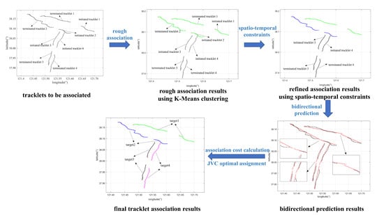
4.2.2. Analysis of Tracklet Association Results

The selected tracklets in Figure 6 were used for tracklet association tests. Firstly, the preliminary tracklet association results using k-means clustering are shown in Figure 8a, and the preliminary tracklets that are classified into one cluster are depicted using the same color and marker. The results show that the initiated tracklets 1 and 2 and the terminated tracklets 1 and 2 are classified into the same cluster, while the initiated tracklets 3 and 4 and terminated tracklets 3 and 4 are placed into the same category.
Then the spatial and temporal constraints were applied to the preliminary associated tracklets to produce the candidate tracklet pairs, as shown in Figure 8b. After this step, the initiated tracklet 1 is associated with the terminated tracklet 1, while the initiated tracklet 2 is associated with the terminated tracklet 2; they are successfully distinguished and depicted in green and blue, respectively. However, the association results of the initiated tracklets 3 and 4 and terminated tracklets 3 and 4 remain the same.
Subsequently, bidirectional prediction was implemented on the candidate tracklets to produce the predicted states, the obtained results are shown as red lines in Figure 9, and the prediction results for the fragmentation parts are zoomed in for a better view. It can be seen that the initiated tracklet 1 and terminated tracklet 1, as well as the initiated tracklet 2 and terminated tracklet 2, can be easily associated, correspondingly. However, association ambiguities still exist in the initiated tracklets 3 and 4 and terminated tracklets 3 and 4 due to their similar headings and speeds.
In order to resolve the association ambiguity of the initiated tracklets 3 and 4 and terminated tracklets 3 and 4, the association costs between possible tracklet pairs were calculated using Equation (31) and listed in Table 3.
Finally, the optimal assignment method based on the JVC algorithm was applied to the association cost matrix of the candidate tracklet pairs to produce the final tracklet association results, as shown in Figure 10. The associated tracklet pairs for the same target are shown in the same colors. It is shown that the tracklets are correctly matched for both target 3 and target 4 with a minimum total association cost of 0.7176 = 0.6052 + 0.1124.

4.2.3. Analysis of Association Accuracy and Computational Complexity

To test the computational efficiency and association accuracy of the proposed method, the correct association rate R t , false association rate R f , and missing association rate R n are defined in Equations (42)–(44), respectively.
R t = n t n u m
R f = n f n u m
R n = n n n u m
where n u m is the total number of tracklets, n t , n f , and n n denote the numbers of correctly associated tracklets, incorrectly associated tracklets, and missed associated tracklets, respectively.
The converted measurement Kalman filter was applied to the field HFSWR data introduced in Section 4.2, first to produce target tracklets, and 51 pairs of tracklets were selected for tracklet association tests. It was verified that each tracklet pair was from the same target by associating them with the same AIS track using the track-to-track association method in [24]. Then, both the proposed multi-stage tracklet association method and the track segment association method in [12] were applied to these 51 tracklet pairs to produce the tracklet association results. The correct association rate R t , false association rate R f , and missing association rate R n were calculated and the obtained results are listed in Table 4. Moreover, in order to evaluate the computational efficiency, the proposed method and the track segment association method in [12] were run 200 times, and the average running time was calculated, respectively; the corresponding results are also listed in Table 4.
It can be seen from the results in Table 4 that, compared with the TSA method in [12], the correct association rate of the proposed method is improved by 30.1%, while its false association rate and missing association rate are reduced by 15.2% and 14.9%, respectively. The average running time of the proposed method is 7.1 s less than that of the TSA method in [12].

5. Discussion

From the above analysis and experimental results, it can be summarized that:
(i) Track fragmentation often occurs during target tracking with compact HFSWR due to its physical limits. Tracklet association methods can connect the broken track segments belonging to a same target, enhancing the tracking continuity.
(ii) The proposed multi-stage tracklet association method provides a “coarse-to-fine” way to match the same target’s tracklets, both accurately and efficiently, which has been verified by experimental results using both simulated and field data with respect to the correct association rate, false association rate, missing association rate, and average running time.
(iii) The rough tracklet association using k-means clustering and tracklet pair refinement by spatiotemporal constraint help to find the possible tracklet pairs. As the tracklets that cannot be associated with any other tracklet have been excluded for further analysis, on the one hand, the computational burden is reduced; on the other hand, the association accuracy can be improved.
(iv) Taking the low positioning accuracy of compact HFSWR into consideration, bidirectional prediction and a global optimal assignment based on JVC resolve the association ambiguities for close tracklets and improve the association accuracy.

6. Conclusions

Track fragmentation is a common problem for target tracking with a compact high-frequency surface wave radar since it degrades the tracking continuity and maritime surveillance performance. In this article, the tracklet association problem for compact HFSWR was investigated and a multi-stage tracklet association method, which consists of rough association using k-means clustering, refinement by spatiotemporal constraint, bidirectional prediction followed by optimal assignment based on JVC algorithm, was developed to repair the broken tracklets. The advantages of the proposed two-stage method are two-fold. In the first stage, k-means clustering can find the possible tracklet pairs efficiently, while the spatiotemporal constraint excludes the tracklet pairs that cannot be associated; thus, the computational efficiency for tracklet association is significantly improved. In the second stage, bidirectional state prediction and the optimal assignment based on the JVC algorithm are able to enhance the tracklet association accuracy under low positioning accuracy and multi-target tracking scenarios. Experimental results with both simulated and field data demonstrate that the proposed method is effective and able to resolve association ambiguities for similar tracklets and improve the track integrity; the association performance is superior to that of the existing track segment association method with a correct association rate improved by 30%.
Low detection probability and low spatial resolution are two main factors leading to track fragmentation for the compact high-frequency surface wave radar. On the one hand, more advanced tracklet association methods should be developed with detection characteristics of a compact high-frequency surface wave radar fully considered. On the other hand, a networking observation with multiple radars is a potential way to improve the target detection probability and positioning accuracy. Moreover, the proposed method should be extended to be applicable to the case involving maneuvering targets.

Author Contributions

Conceptualization, W.S.; methodology, W.S. and P.M.; software, P.M. and Z.P.; validation, W.S., W.H. and Y.J.; formal analysis, W.S. and W.H.; investigation, Z.P.; resources, Y.J. and Y.D.; data curation, Y.J.; writing—original draft preparation, W.S. and Z.P; writing—review and editing, W.H., W.S. and X.L.; visualization, X.L.; supervision, W.H. and Y.D.; project administration, W.S.; funding acquisition, W.S. All authors have read and agreed to the published version of the manuscript.

Funding

This research was funded by the National Natural Science Foundation of China with grant numbers 62071493, 61831010, the Fundamental Research Funds for the Central Universities with grant number 19CX02046A.

Data Availability Statement

The data and the code of this study are available from the corresponding author upon request ([email protected]).

Acknowledgments

The authors would like to thank the anonymous reviewers for their comments and suggestions, which helped to improve the quality of this article.

Conflicts of Interest

The authors declare no conflict of interest.

Abbreviations

HFSWRhigh-frequency surface wave radar
CORMScompact over-the-horizon radar for maritime surveillance
CITcoherent integration time
TSAtrack segment association
JVCJonker–Volgenant–Castanon
FMICWfrequency modulated interrupted continuous wave
CFARconstant false alarm rate
DOAdirection of arrival
MUSICmultiple signal classification
DBFdigital beamforming
CMKFconverted measurement Kalman filter
SNRsignal-to-noise ratio
SCRsignal-to-clutter ratio
AISautomatic identification system

References

  1. Sun, W.; Pang, Z.; Huang, W.; Ji, Y.; Dai, Y. Vessel velocity estimation and tracking from Doppler echoes of T/R-R composite compact HFSWR. IEEE J. Sel. Top. Appl. Earth Obs. Remote Sens. 2021, 14, 4427–4440. [Google Scholar] [CrossRef]
  2. Ji, Y.; Zhang, J.; Wang, Y.; Sun, W.; Li, M. Target monitoring using small-aperture compact high-frequency surface wave radar. IEEE Aerosp. Electron. Syst. Mag. 2018, 33, 22–31. [Google Scholar] [CrossRef]
  3. Park, S.; Cho, C.J.; Ku, B.; Lee, S.; Ko, H. Compact HF surface wave radar data generating simulator for ship detection and tracking. IEEE Geosci. Remote Sens. Lett. 2017, 14, 969–973. [Google Scholar] [CrossRef]
  4. Roarty, H.J.; Rivera Lemus, E.; Handel, E.; Glenn, S.M.; Barrick, D.E.; Isaacson, J. Performance evaluation of SeaSonde high-frequency radar for vessel detection. Mar. Technol. Soc. J. 2011, 45, 14–24. [Google Scholar] [CrossRef]
  5. Smith, M.; Roarty, H.; Glenn, S.; Whelan, C.; Barrick, D.; Isaacson, J. Methods of associating CODAR SeaSonde vessel detection data into unique tracks. In Proceedings of the 2013 OCEANS, San Diego, CA, USA, 23–27 September 2013; pp. 1–5. [Google Scholar]
  6. Lu, B.; Wen, B.Y.; Tian, Y.W.; Wang, R.K. A vessel detection method using compact-array HF radar. IEEE Geosci. Remote Sens. Lett. 2017, 14, 2017–2021. [Google Scholar] [CrossRef]
  7. Zhou, H.; Roarty, H.; Wen, B.Y. Wave extraction with portable high-frequency surface wave radar OSMAR-S. Ocean Univ. China 2014, 13, 957–963. [Google Scholar] [CrossRef]
  8. Helzel, T.; Hansen, B.; Kniephphoff, M.; Petersen, L.; Valentin, M. Introduction of the compact HF radar WERA-S. In Proceedings of the IEEE/OES Baltic International Symposium, Klaipeda, Lithuania, 8–10 May 2012; pp. 1–3. [Google Scholar]
  9. Roarty, H.J.; Barrick, D.E.; Kohut, J.T.; Glenn, S.M. Dual-use of compact HF radars for the detection of mid- and large-size vessels. Turk. J. Electr. Eng. Comput. Sci. 2010, 18, 373–388. [Google Scholar]
  10. Sun, W.; Huang, W.; Ji, Y.; Dai, Y.; Ren, P.; Zhou, P.; Hao, X. A vessel azimuth and course joint re-estimation method for compact HFSWR. IEEE Trans. Geosci. Remote Sens. 2020, 58, 1041–1051. [Google Scholar] [CrossRef]
  11. Sun, W.; Huang, W.; Ji, Y.; Dai, Y.; Ren, P.; Zhou, P. Vessel tracking with small-aperture compact high-frequency surface wave radar. In Proceedings of the MTS/IEEE Oceans, Marseille, France, 17–20 June 2019; pp. 1–4. [Google Scholar]
  12. Yeom, S.W.; Kirubarajan, T.; Bar-Shalom, Y. Track segment association, fine-step IMM and initialization with Doppler for improved track performance. IEEE Trans. Aerosp. Electron. Syst. 2004, 40, 293–309. [Google Scholar] [CrossRef]
  13. Bar-Shalom, Y.; Kirubarajan, T.; Gokberk, C. Tracking with classification-aided multiframe data association. IEEE Trans. Aerosp. Electron. Syst. 2005, 41, 868–878. [Google Scholar] [CrossRef]
  14. Li, X.R.; Jilkov, V.P. Survey of maneuvering target tracking. Part I. Dynamic models. IEEE Trans. Aerosp. Electron. Syst. 2003, 39, 1333–1364. [Google Scholar]
  15. Zhang, S.; Bar-Shalom, Y. Track segment association for GMTI tracks of evasive move-stop-move maneuvering targets. IEEE Trans. Aerosp. Electron. Syst. 2011, 47, 1899–1914. [Google Scholar] [CrossRef]
  16. Pan, S.S.; Bao, Q.L.; Hou, W.B.; Che, Z.P. An improved track segment association algorithm using MM-GNN method. In Proceedings of the 2017 Progress in Electromagnetics Research Symposium Spring—(PIERS), St. Petersburg, Russia, 22–25 May 2017; pp. 675–681. [Google Scholar]
  17. Raghu, J.; Srihari, P.; Tharmarasa, R.; Kirubarajan, T. Comprehensive track segment association for improved track continuity. IEEE Trans. Aerosp. Electron. Syst. 2018, 54, 2463–2480. [Google Scholar] [CrossRef]
  18. Hong, S.X.; Peng, D.L.; Shi, Y.F. Track-to-track association using fuzzy membership function and clustering for distributed information fusion. In Proceedings of the 37th Chinese Control Conference, Wuhan, China, 25–27 July 2018; pp. 4028–4032. [Google Scholar]
  19. Zhu, Y.Q.; Zhou, S.L.; Gao, G.; Ji, K.F. Emitter Target Tracking by Tracklet Association Using Affinity Propagation. IEEE Sens. J. 2015, 15, 5645–5653. [Google Scholar] [CrossRef]
  20. Shao, H.; Japkowicz, N.; Abielmona, R.S. Vessel track correlation and association using fuzzy logic and Echo State Networks. In Proceedings of the 2014 IEEE Congress on Evolutionary Computation (CEC), Beijing, China, 6–11 July 2014; pp. 2322–2329. [Google Scholar]
  21. Zhang, L.; Mao, D.W.; Niu, J.; Wu, J.; Ji, Y.G. Continuous Tracking of Targets for Stereoscopic HFSWR Based on IMM Filtering Combined with ELM. Remote Sens. 2020, 12, 272. [Google Scholar] [CrossRef] [Green Version]
  22. Sun, W.; Ji, M.; Huang, W.; Ji, Y.; Dai, Y. Vessel tracking using bistatic compact HFSWR. Remote Sens. 2020, 12, 1266. [Google Scholar] [CrossRef] [Green Version]
  23. Bar-Shalom, Y.; Willett, P.; Tian, X. Tracking and Data Fusion: A Handbook of Algorithms; YBS Publishing: Storrs, CT, USA, 2011. [Google Scholar]
  24. Nikolic, D.; Stojkovic, N.; Lekic, N. Maritime over the horizon sensor integration: High frequency surface-wave-radar and automatic identification system data integration algorithm. Sensors 2018, 18, 1147. [Google Scholar] [CrossRef] [Green Version]
  25. Xiao, J.Z.; Li, X. A Research of the Partition Clustering Algorithm. In Proceedings of the 2010 International Symposium on Intelligence Information Processing and Trusted Computing, Huanggang, China, 28–29 October 2010; pp. 551–553. [Google Scholar]
  26. Jonker, R.; Volgenant, A. A shortest augmenting path algorithm for dense and sparse linear assignment problems. Computing 1987, 38, 325–340. [Google Scholar] [CrossRef]
  27. Kadar, I.; Eadan, E.R.; Gassner, R.R. Comparison of robustized assignment algorithms. In Proceedings of the Aerospace Defence Sensing and Control (Aero Sense) Conference, Orlando, FL, USA, 21–25 April 1997; Volume 3068, pp. 240–249. [Google Scholar]
  28. Bordonaro, S.; Willett, P.; Bar-Shalom, Y. Decorrelated unbiased converted measurement Kalman filter. IEEE Trans. Aerosp. Electron. Syst. 2014, 50, 1431–1444. [Google Scholar] [CrossRef]
Figure 1. An illustrative comparison between the instantaneous heading and average heading.
Remotesensing 14 01601 g001
Figure 2. Analysis of the instantaneous headings. (a) The tracklet examples. (b) The estimation results of instantaneous headings.
Remotesensing 14 01601 g002
Figure 3. The flowchart of the multi-stage tracklet association method.
Remotesensing 14 01601 g003
Figure 4. Tracking results using the simulated data.
Remotesensing 14 01601 g004
Figure 5. Tracklet association results. (a) The TSA method in [12]. (b) The proposed method.
Remotesensing 14 01601 g005
Figure 6. Tracklets from field data for the association test.
Remotesensing 14 01601 g006
Figure 7. Tracklets illustration. (a) Tracklets of target 1. (b) Tracklets of target 2.
Remotesensing 14 01601 g007
Figure 8. Intermediate association results of the proposed method. (a) Rough association results using k-means clustering. (b) Association results after spatiotemporal constraints.
Remotesensing 14 01601 g008
Figure 9. Bidirectional prediction results.
Remotesensing 14 01601 g009
Figure 10. Final tracklet association results.
Remotesensing 14 01601 g010
Table 1. Initial parameters of simulated targets.
Initial Range (km)Initial Azimuth ()Initial Doppler Velocity (km/h)
Target 1107−1022
Target 2106−1121
Target 374−7−19
Target 4112−8−23
Target 593−7−19
Table 2. Association costs between different tracklet combinations of target 1 and target 2.
Terminated TrackletTerminated Tracklet 1Terminated Tracklet 2
Initiated Tracklet
Initiated Tracklet 10.11170.0228
Initiated Tracklet 20.70200.5933
Table 3. Association costs between tracklet pairs of target 3 and target 4.
Terminated TrackletTerminated Tracklet 3Terminated Tracklet 4
Initiated Tracklet
Initiated Tracklet 30.60520.1577
Initiated Tracklet 40.71730.1124
Table 4. Performance comparisons between two tracklet association methods.
R t  (%) R f  (%) R n  (%)Average Running Time (s)
TSA method in [12]63.419.517.110.4
Proposed Method93.54.32.23.3
Publisher’s Note: MDPI stays neutral with regard to jurisdictional claims in published maps and institutional affiliations.

