An Approach to Semantically Segmenting Building Components and Outdoor Scenes Based on Multichannel Aerial Imagery Datasets

Abstract

As-is building modeling plays an important role in energy audits and retrofits. However, in order to understand the source(s) of energy loss, researchers must know the semantic information of the buildings and outdoor scenes. Thermal information can potentially be used to distinguish objects that have similar surface colors but are composed of different materials. To utilize both the red–green–blue (RGB) color model and thermal information for the semantic segmentation of buildings and outdoor scenes, we deployed and adapted various pioneering deep convolutional neural network (DCNN) tools that combine RGB information with thermal information to improve the semantic and instance segmentation processes. When both types of information are available, the resulting DCNN models allow us to achieve better segmentation performance. By deploying three case studies, we experimented with our proposed DCNN framework, deploying datasets of building components and outdoor scenes, and testing the models to determine whether the segmentation performance had improved or not. In our observation, the fusion of RGB and thermal information can help the segmentation task in specific cases, but it might also make the neural networks hard to train or deteriorate their prediction performance in some cases. Additionally, different algorithms perform differently in semantic and instance segmentation.

1. Motivation and Introduction

Researchers are exploring an efficient energy loss audit approach for groups of buildings in large districts, since buildings are mutually affected. Recently, with the support of thermal cameras, it has become possible to detect energy loss from a building’s facade and roof by reading the temperature information from thermal images [1,2]. This approach originally motivated researchers to detect energy loss from an entire building using a handheld thermal camera [2,3]. Due to the time required, it is not feasible to detect energy loss from all buildings in a whole district using such a handheld camera. To improve efficiency, researchers have mounted cameras and multiple sensors on unmanned aircraft systems (UASs). This solution allows for faster data collection and broader camera views [4]. However, the thermal information from other objects—such as cars and equipment—is also captured, which is not the type of heat loss that we focus on. For example, Xu et al. [5] and Friman et al. [6] used UAS-based thermal images to detect heat loss from district heating networks; however, they had to distinguish road objects from others, since heat loss from cars and equipment is also captured in UAS-based thermal images. Similarly, in order to better detect the source(s) of energy loss, we need to be able to differentiate between buildings’ various components and other items in the scene—and, further, to determine whether the energy loss is from a particular building [7]. To differentiate components’ semantic information (semantic segmentation) and to delineate each distinct object (instance segmentation), many computer vision algorithms—especially deep learning approaches—have been developed, such as Mask R-CNN [8], the YOLO family [9], and the DeepLab family [10]. These segmentation algorithms allow for object detection at the pixel level and indexing of each distinct object, thus enabling the classification of each image pixel.

Traditional semantic segmentation is primarily based on visible-light imagery input—also known as red–green–blue (RGB) images—which makes the task intrinsically challenging [11,12]. For example, it is difficult to precisely distinguish between objects of similar colors. To overcome this limitation of RGB data and further improve the performance of semantic segmentation, other forms of measurement can be used in addition to RGB images, such as depth and thermal information. Unlike visible light imaging, thermal imaging cameras can detect objects’ thermal information under various lighting conditions, and even under difficult conditions such as night-time. Therefore, adding thermal information helps some applications that require high segmentation precision [13,14].

In our semantic segmentation task, we focused on differentiating salient components—such as facades and roofs—where energy loss was important to monitor, as well as on peripheral components such as cars and equipment, where heat loss was not our main focus, but may interfere in the study. Therefore, in this research, we classified the five most relevant categories of classes: facades, roofs, cars, roof equipment, and ground equipment. Researchers have implemented similar methods to detect thermal anomalies while reducing the false positive rate—the ratio between the number of negative samples wrongly categorized as positive and the total number of actual negative samples. For example, Berg et al. [15,16] used thresholds to classify whether pixels in images belonged to a building or not. Friman et al. [6] analyzed the distribution of pixel intensities across thermal images, and set a temperature threshold to distinguish buildings from the ground. However, setting a threshold and simply determining whether heat loss is from buildings—as opposed to cars and ground equipment—without the support of semantic information is not possible. Therefore, we need to define a framework that can directly conduct segmentation on aerial RGB datasets, thereby adding multiple channels that can potentially improve segmentation performance.

Our study was designed to answer the following questions: (1) How do thermal images influence the performance of semantic and instance segmentation? (2) Can thermal information be fused with RGB information to improve the performance of semantic segmentation? If so, how can such fusion be supported by different approaches? (3) How do DCNNs perform for different categories of classes? Our study contributes a Building Object and Outdoor Scene Segmentation (BOOSS) database to building science research. In this dataset, a collection of aerial imagery data fusing thermal and RGB information with annotations of building components and other classes are provided. Additionally, our study uses multichannel imagery data to solve the building component segmentation problems for energy audits. The rest of this paper is organized into the following sections: Section 2 reviews the existing works in the field. Section 3 presents the methodology of this study. Section 4 presents case studies and results, while Section 5 concludes the paper and presents potential future work.

2. Related Work

2.1. Energy Aduits

Energy audits on building envelopes are important for building performance, and increasing the efficiency of building envelopes is a low-cost but high-return strategy [17]. Lucchi [18] reviewed studies that used thermal cameras to solve energy audit problems based on qualitative and quantitative approaches. Qualitative approaches include (1) classification of building components [19], (2) thermal bridge identification [20,21], (3) air leakage inspection [22], and (4) HVAC and pipeline system inspection [23]. Quantitative approaches include (1) U-value assessment [24,25], (2) moisture content identification [26], (3) thermal anomaly percentage calculation [16], and (4) indoor occupancy calculation for energy consumption inspection [27]. Recently, researchers have also installed thermal cameras onto other devices, such as unmanned aerial vehicles (UAVs) [28] and unmanned ground vehicles (UGVs) [29], to capture thermal images. When researchers used a handheld data collection approach, they were informed of what objects they investigated. However, for energy audits using an aerial-based data collection approach, researchers need to distinguish objects before processing thermal information, because aerial-based data collection captures all information, including regions of interest and outliers alike. For example, Friman et al. [6] and Berg et al. [15,16] inspected heat loss from district heating networks; they needed to differentiate road components; otherwise, heat information captured from cars and building roofs could influence the energy audit accuracy. Therefore, a building component segmentation procedure is required for energy audits.

2.2. Neural Network Approaches for Feature Extraction

Traditional feature extraction approaches have been classified as either appearance-based or part-based [30]. Appearance-based approaches include principal component analysis (PCA) [31,32], linear discriminant analysis (LDA) [33,34], and independent component analysis (ICA) [35]. The part-based approaches mainly include scale-invariant feature transformation (SIFT) [36], and its variants: PCA–SIFT [37] and gradient location–orientation histogram (GLOH) [38].

The traditional approaches, as previously summarized, are all linear processing approaches. Another approach, created by the fast development of deep neural networks for feature extraction, is the convolutional neural network (CNN). In classic CNN models, convolution and fully connected (FC) layers implement linear transformations on their inputs. Later, nonlinearity is added to the feature extraction tasks, such as activation and pooling layers.

Among these approaches, Alex Krizhevsky and Geoffrey Hinton’s AlexNet CNN can be considered the most interesting work after a long hiatus in the computer vision neural network research [39], because of its special network architecture. Many deep neural network architectures have been designed based on this work, such as ZFNet [40] and VGGNet. In particular, VGGNet significantly outperforms other networks. The biggest difference between VGGNet and others is the size of its filters. Both AlexNet and ZFNet use large filters—11 × 11 [39] and 7 × 7 [40], respectively—but VGGNet reduces the parameters by using two layers of 3 × 3 filters (equivalent to a filter of 5 × 5) or three layers of 3 × 3 filters (equivalent to a filter of 7 × 7). As there are fewer parameters to learn, VGGNet can converge faster and avoid overfitting problems. There are many different versions of VGGNet, but the most popular are VGG-16 and VGG-19, because of their accuracy and learning speed.

Another interesting architecture is GoogLeNet, which makes networks much deeper. This deeper network is defined as “inception”. The first GoogLeNet technique introduced a 1 × 1 convolution as a dimension-reduction module by reducing the computation bottleneck, thereby allowing for an increase in the network depth and width. It has also been demonstrated that this technique can reduce the overfitting problem, because the technique has a regularization effect. The second GoogLeNet technique involves the FC layers, which are different from other networks’ architectures, wherein whole feature maps are fully connected to each FC layer. In GoogLeNet, global average pooling is obtained by averaging each individual element of the feature maps to each related FC layer element. These two techniques allow GoogLeNet layers to reach 22 layers in total, which is very deep compared with AlexNet, ZFNet, and VGGNet.

However, deeper neural networks also have drawbacks. For example, it is known that the deeper layers may cause the problems of a vanishing or exploding gradient. To solve these problems, a ship connection (or shortcut connection) is implemented in a ResNet architecture by adding an input layer to the output layer after a few skipped layers. To reduce the computational complexity, ResNet also uses a bottleneck design technique, which adds an extra 1 × 1 convolutional layer to the network’s beginning and end. Despite the increases in layer size, there is no additional complexity. For instance, ResNet-152 is still less complex than VGG-16/19.

2.3. Semantic Segmentation

Segmentation has many different prototypes with different architectural designs. To better understand their performance, we compared the most utilized frameworks, including the fully connected network (FCN) [41,42], the pyramid scene parsing network (PSPNet) [43], DeepLab v3+ [10,44], and Mask R-CNN [8]. According to the commonly used website Paper with Code, in which researchers compete for the best performance [45], these algorithms are highly ranked and, thus, are included in this literature review.

First, the FCN is derived from classic object detection approaches, in which input images are downsized and fed into the convolution and fully connected (FC) layers, and the output predicts object labels. If the output is upsampled to a pixel-wise output rather than a single label, it can be used to predict semantic information. Second, PSPNet uses a pyramid parsing module that exploits global context information in the network. This module utilizes different region-based context aggregation, and its final prediction is more reliable than the FCN because of the collection of both local and global clues. PSPNet first extracts a feature map from the input image. On the top of the map, it aggregates context information using a four-level pyramid pooling module. The kernels of this pooling module cover the whole image, half the image, and small portions. After pooling, this context information is concatenated with the original feature map in the final part. Lastly, the final prediction is generated from a succeeding convolutional layer. Next, DeepLab v3+ is the third version in the DeepLab family developed by Google, which conducts segmentation tasks directly on the input images. Compared with traditional convolutional layers that process all neighboring values together, the DeepLab family uses dilated convolutions (also known as atrous convolutions), by which certain input values are skipped in order to observe a greater field of view. This technique allows filters to include more context using fewer parameters [10]. Both the first and second versions of DeepLab use an atrous convolution and a fully connected conditional random field (CRF), and the second version has one additional technique—atrous spatial pyramid pooling (ASPP), in which multiple parallel atrous convolutions with different rates are fused to generate a feature map. Following the success of v1 and v2, Google proposed v3 and v3+ by removing the CRF but reconstructing the ASPP, improving performance [46]. Lastly, Mask R-CNN extends the Faster R-CNN by adding a new branch that can predict an object mask. Unlike semantic segmentation, which assigns every pixel of an image with a class label, Mask R-CNN, as a form of instance segmentation, treats multiple objects of the same class as distinct individual instances; it first proposes candidate regions of interest (ROIs) using a region proposal network (RPN), and then extracts feature maps, applying pooling and other convolutional neural networks to these regions. Mask R-CNN uses these regions to define bounding boxes and identify individual items in the same class.

The abovementioned algorithms are not the only approaches. There are many other algorithms of both semantic and instance segmentation. The difference between semantic and instance segmentation is that semantic segmentation treats multiple objects of the same category as a whole entity, while instance segmentation treats multiple objects of the same class as distinct individual instances. The other semantic algorithms include UNet [47], a context-guided network (CGNet) [48], and unified perceptual parsing (UPerNet) [49]. UNet is a basic segmentation approach that was frequently used before complex CNN approaches were implemented; its performance accuracy has been surpassed by many current approaches. CGNet has fewer network parameters and, thus, its training process is faster but less accurate compared to PSPNet and DeepLab v3+. UPerNet is very similar to PSPNet, and they achieve similar performances.

The other instance segmentation approaches include the YOLO family and the Faster-RCNN family. Similar to Mask R-CNN, the other instance segmentation algorithms use similar techniques. However, such algorithms only predict bounding boxes for objects, and do not assign pixel-wise classes to objects in the bounding boxes.

2.4. Current Datasets

There are many datasets for semantic segmentation research in the computer vision field, such as Cityscapes, PASCAL visual object classes (VOC), ADE20K, and ScanNet. Cityscapes is designed to identify semantic information on urban street scenes. Many classified objects include vehicles, trees, and signal signs. These images are generally taken from the ground. PASCAL VOC, on the other hand, can detect over 400 miscellaneous objects from datasets. ADE20K includes many objects, such as food, furniture, and appliances in indoor scenes, and vehicles, infrastructure, and buildings in outdoor scenes, with over 250 annotated instances. ScanNet provides an annotated 3D reconstruction of indoor scenes. These datasets are all RGB imagery datasets.

There are several different types of open-source dataset with multiple channels, such as Kinect data, simultaneous localization and mapping (SLAM) data, and synthetic data. These datasets fuse RGB information with depth information to improve segmentation accuracy. However, after reviewing current open-source datasets, we found that there are no outdoor scene datasets in which detailed images of facades, roofs, windows, etc., are included for building envelope energy audits. Additionally, the aforementioned open-source datasets are usually collected using ground-based equipment. Such data acquisition methods do not allow for building roof inspections. Mayer et al. [50] recently published a hyperspectral database (RGB + thermal + height) with drone images for thermal bridge detection; however, their datasets only focused on roof components, without other objects in an outdoor scene.

To comprehensively inspect building envelopes in an urban area with several structures, it is necessary to collect drone-based aerial images of buildings and outdoor scenes. In this study, we implemented experiments on our collected and processed datasets, called Building Object and Outdoor Scene Segmentation (BOOSS)—Aerial Imagery Datasets. The images were taken in the winter in Karlsruhe, Germany. The outdoor temperature was −5 °C (23 °F) when we conducted our experiments. Since another use case of the dataset was to detect heat loss from the thermal images, we avoided sunny days in order to eliminate the impact of solar radiation on building envelopes.

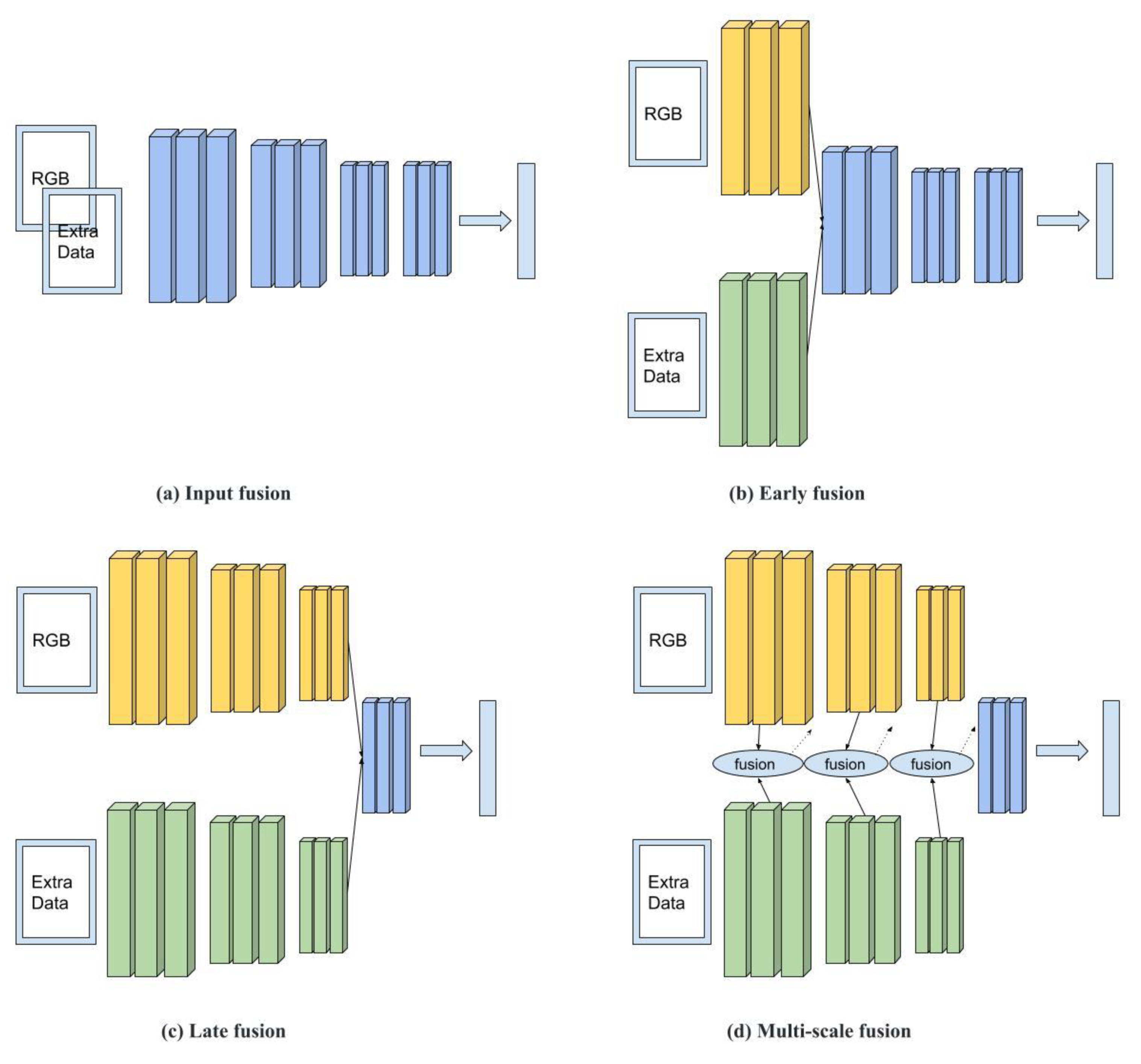
2.5. Image Data Fusion and Related Work

Researchers have found that fusing multiple sensor data with RGB data can potentially improve object classification performance [51,52,53]. Commonly used fusion approaches can be categorized into four types: input, early, late, and multiscale fusion. As shown in Figure 1a, RGB and data provided by an extra channel (e.g., depth, thermal, or other types) are integrated as joint inputs fed into a neural network. This fusion approach is called input fusion. As shown in Figure 1b,c, the RGB and extra channel data are first fed into different network streams, where their features are then extracted by the lower level or the upper level and combined as joint features for the next-level decision. These fusion approaches are called early and late fusion, respectively. In multiscale fusion, as shown in Figure 1d, the RGB and extra data are separately fed into two streams. Unlike late fusion, in which the extracted features (yellow blocks and green blocks) are connected in the last step, the multiscale fusion process in Figure 1d takes place in every step.

RGB–Depth Fusion: The studies conducted by Ren et al. [54] and Peng et al. [55] are examples of input fusion, in which RGB and depth images were directly concatenated to form a four-channel input. Qu et al.’s [56] work is an early fusion method, while studies by Desingh et al. [57] and Wang et al. [58] are examples of late fusion methods. Many studies also work on multiscale fusion; for example, Chen et al. [53] used paired RGB and depth images to implement segmentation. Their neural networks were examples of late fusion but, in contrast, they built connections between the final layer (the blue block in Figure 1d) and every early layer (every yellow block and green block), which they called cross-modal interaction. Their approach took every neural network layer into account when making a prediction on the last layer. Chen and Li [52] conducted a similar work, but the difference was that they first concatenated the RGB feature network stream (the yellow blocks in Figure 1d) with the depth feature stream (the green blocks in Figure 1d), and fused the concatenated features, the last RGB features, and the last depth features to make a final prediction.

In addition to changing the RGB network structures and depth fusion models, researchers have also explored methods to use synthetic depth images due to data hunger, which refers to a shortage of paired RGB–depth data required for training a segmentation model [59]. These paired RGB–depth images are usually rendered from a 3D virtual environment rather than sensors in the real world, which can save ground-truth labeling time. For example, Chen et al. [60] used a 3D scene generator and a 2D rendering engine to simulate RGB images and depth maps for the ground, buildings, and trees with their corresponding annotations. Since the model can be easily adjusted in a 3D virtual environment, the annotations for different objects only need to be configured once, and all of the RGB and depth images can then be rendered along with their annotated objects. Similarly, Chen et al. also implemented their synthetic methods on campuses [61] and in urban areas [62].

RGB–Thermal Fusion: Thermal data are another data type that can be used to improve semantic segmentation [63]. For example, Laguela et al. [64] researched how to generate a high-quality thermographic image of a building envelope by fusing infrared data with RGB images. Similarly, Luo et al.’s [65] hybrid tracking framework is an early fusion method. Conversely, Li et al.’s [66] two-stream CNN of RGB–thermal object tracking is a typical late fusion method. Additionally, researchers have also implemented multiscale fusion methods such as Zhai et al.’s [67] cross-modal correlation filters and Jiang et al.’s [68] cross-modal multi-granularity attention networks. As illustrated in Figure 1d, the classic approach builds one stream for RGB and another for extra data, but Jiang et al. [68] built two streams for RGB data and two for thermal data. The authors fused the four streams to a make final prediction. The benefit of their method is that they learned more features from data, but it also increased the computational burden. Researchers have similarly explored using synthetic data for RGB–thermal segmentation. For example, Hou et al. [20] used a generative adversarial network (GAN) to simulate building envelope thermal images based on RGB images. Researchers have also fused multiple data types; for example, Mayer et al. [69] combined thermal, depth, and RGB data in their thermal bridge detection studies.

Feature–Feature Fusion: For feature–feature data fusion, researchers have not used multiple sensor data, but they have built multiple neural network channels with different feature extraction methods. They next fused multiple extracted feature channels into one channel and implemented the segmentation process. These methods fuse multiple feature channels extracted from original RGB images instead of fusing multiple channels recorded by different sensors. Nevertheless, their fusion methods provide alternative solutions to segmentation problems. For example, Nawaz et al. [51] built attention map networks (AMNs) in addition to traditional feature extraction methods to subtract background information from RGB images. In their method, the attention map is a mechanism that extracts different weights from original RGB images.

Since each dataset that computer vision tasks use has many object classes, algorithms usually calculate a total accuracy over all classes, and we cannot evaluate their performances when analyzing an individual object class. For our building envelope inspection purpose, it is necessary to investigate an algorithm’s performance for different object classes, so that building owners, urban planners, and district managers can correspondingly audit energy loss.

3. Methodology

3.1. Data Collection

After reviewing current open-source datasets, we did not find useful outdoor scene datasets for building envelope energy audits in the field of civil engineering. Additionally, the existing open-source datasets are usually collected using ground-based equipment. Such data acquisition methods do not allow for the inspection of building roofs and high building facades. To comprehensively inspect building envelopes, we thus need to collect drone-based aerial images of buildings and outdoor scenes. Therefore, in our dataset, we focused on five categories: roofs, facades, roof equipment, cars, and ground equipment.

The images we used were taken with an FLIR Duo Pro R camera that was mounted on the DJI Matrix 600 drone. The FLIR Duo Pro R is one of the most widely used thermal cameras because it has both an RGB lens and a thermal lens packed together; as such, it can take thermal images and RGB images simultaneously. Using these tools, we can detect two types of energy loss: heat loss, and cooling loss. However, if thermal cameras are used for energy loss detection, we can only detect heat loss in the winter (cold seasons), because the required temperature difference (at least 10 °C) between indoors and outdoors can be guaranteed. On the other hand, in the summer (hot seasons), cooling leakages cannot be identified. Therefore, in our studies, the images were taken in Germany during the winter.

In order to explore and understand the performance of our data fusion strategies, as well as using different algorithms, we applied input fusion to three different pioneering segmentation frameworks: PSPNet, DeepLab v3+, and Mask R-CNN. As shown in

Table 1. Evaluation of algorithms, with their global ranks (data source: Papers with code. https://paperswithcode.com/ (accessed on 27 May 2021)).

Model	Testing Dataset	Metric	Global Rank
Mask R-CNN	COCO	Average precision	1st
		Mean average precision	1st
	Cell17	F1 score	2nd
		Dice	2nd
PSPNet	NYU Depth v2	Mean IoU	4th
	Cityscapes	Mean IoU	3rd
DeepLab v3+	PASCAL VOC	Mean IoU	2nd
	SkyScapesDense	Mean IoU	2nd
UPerNet [49]	ADE20K	Mean IoU	45th
UNet [47]	Anatomical Tracings of Lesions After Stroke (ATLAS)	IoU	2nd
	Retinal vessel segmentation	F1 score	10th
CGNet [48]	MSU video super resolution benchmark	Subjective score	21st

, these three algorithms have higher global ranks [45]. UNet has a good performance, but it only works for small images. For example, the dataset ATLAS is a medical image dataset. We used these frameworks to test only on RGB images, and then we revised the frameworks to test datasets that fused thermal and RGB images.

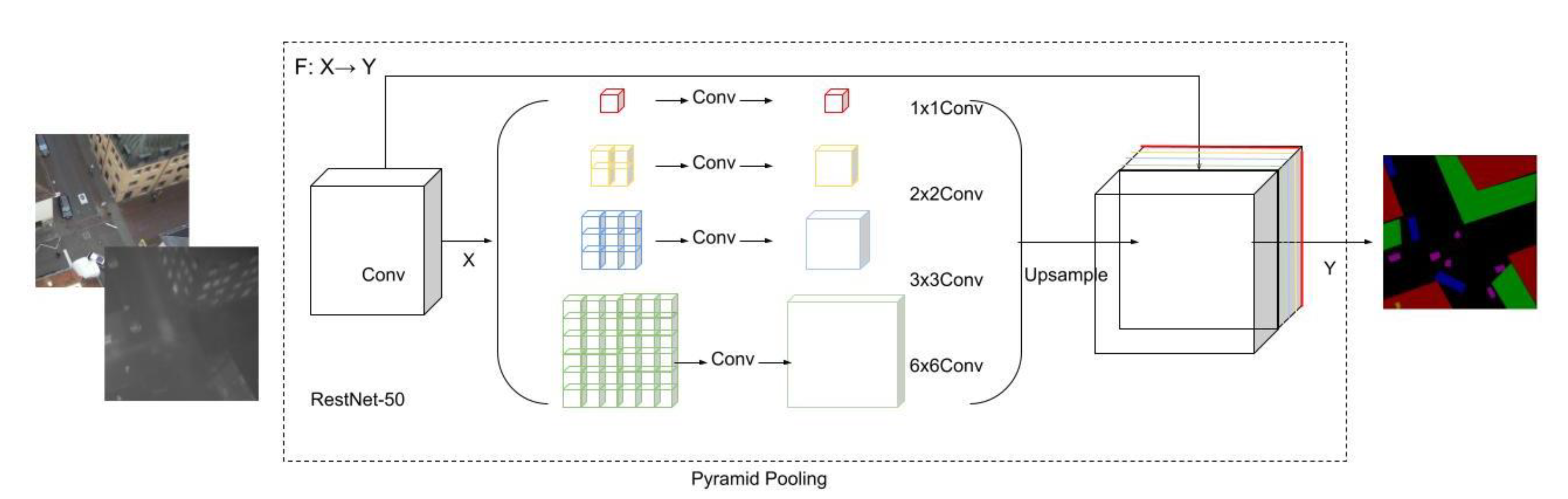
3.2. PSPNet Implementation

The first algorithm we used and adapted was PSPNet [43], as shown in Figure 2. Unlike the FCN, PSPNet does not implement pixel-wise prediction training from a fully connected feature map. In its first stage, the algorithm implements training on a series of feature maps that consist of different filters. This collection of feature maps is defined as a pyramid pooling module. In the second stage, the pooling layers are upsampled and concatenated to former feature maps to generate final feature information, which is later fed into a convolutional layer to obtain the final pixel-wise semantic prediction.

Figure 2 illustrates the input fusion approach on RGB plus thermal datasets using PSPNet. In this algorithm, the loss functions include auxiliary loss and master branch loss. Auxiliary loss allows the optimization of the learning process, while master branch loss is responsible for the whole network. PSPNet adds parameter weights to these two loss functions, including 0.4 for auxiliary loss and 0.6 for master branch loss (a ratio of 4:6 is recommended by the original author).

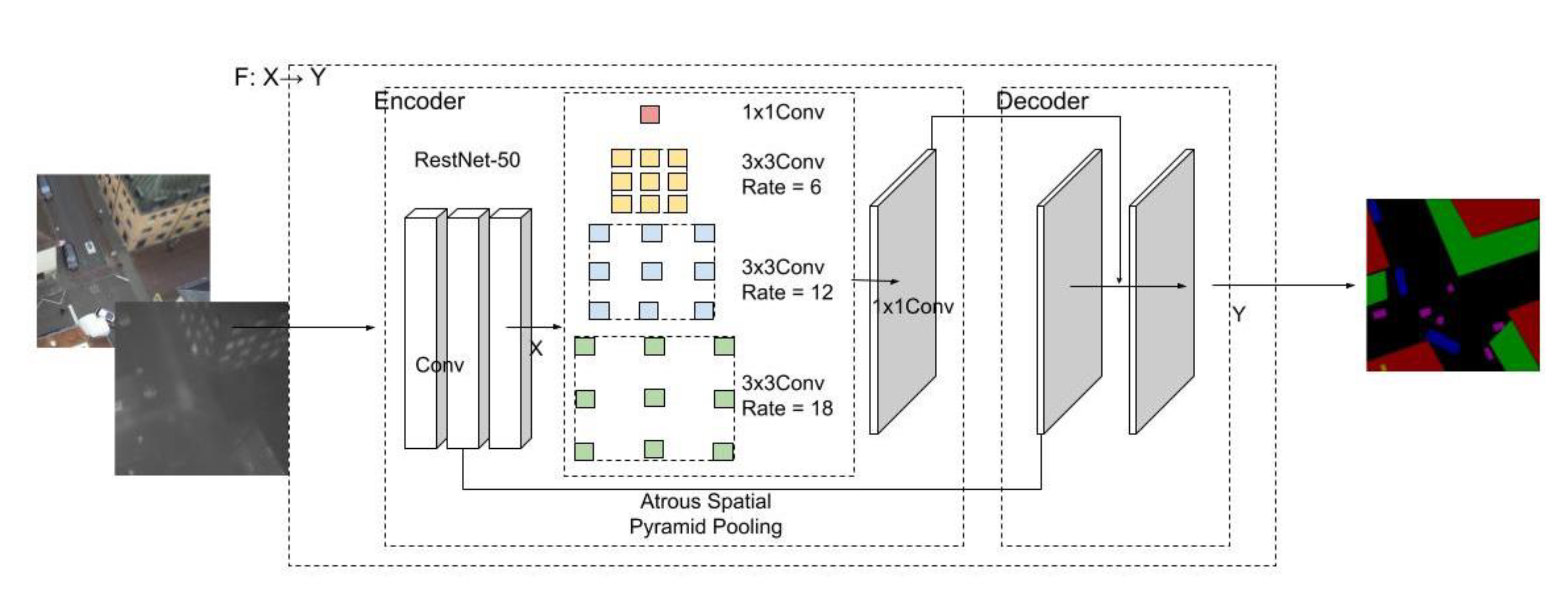
3.3. DeepLab v3+ Implementation

The second tested algorithm was from the DeepLab family [10,44,46]. We used and revised the latest version (DeepLab v3+). DeepLab v3+, as with its other versions, also uses the pyramid pooling method used in PSPNet. However, unlike PSPNet, the DeepLab family uses an innovative pooling structure called atrous spatial pyramid pooling (ASPP). This pooling structure can capture multiscale information by adjusting the filter’s field of view. Unlike using a traditional pooling structure, it also considers the hidden relationship between disconnected pixels in the imagery datasets. Additionally, the several parallel ASPP convolutional layers used in DeepLab v3+ have different rates from the pooling layers used in PSPNet.

The biggest difference between the latest version of DeepLab and earlier versions is that it extends DeepLab v3 by employing an encoder–decoder structure. This structure can expedite computations for feature extraction because it does not enlarge the neural network, and it can also recover sharp segmentation boundaries in the decoder path.

We used ResNet-50 on both the RGB and thermal images for performance comparison, and then the overlapped extracted features for the remaining steps, which are similar to the typical DeepLab v3 approach. Figure 3 illustrates the input fusion approach on DeepLab v3+. First, we simply concatenated a thermal channel after the RGB channels to obtain four-channel input data. To guarantee the performance while using an acceptable computational capacity, we used a 512 × 512 image size, which is commonly used in other applications. Second, the integrated images were fed into the typical DeepLab v3 + network, with the condition that only the first input layer was adjusted from three to four in order to conveniently process the input four-channel images. The loss function of the DeepLab family calculates the sum of cross-entropy terms for each spatial position in their networks, and assigns equal weight to each term.

3.4. Mask R-CNN Implementation

Figure 4 illustrates the input fusion approach on the adapted Mask R-CNN. Formally, the task is defined as follows: given a set $X$ containing input images $x_i\in R^{H\times W\times C}$ with image height $H$, width $W$, and channels $C$ (in this case, the RGB image size is 512 × 512 × 3, so $H$ = 512, $W$ = 512, and $C$ = 3), and a corresponding annotation set $Y$ containing bounding boxes $y_{i,box}\in R^{N\times 4}$, where the number 4 represents the coordinates of a bounding box’s four corners, class labels $y_{i,cls}\in R^N$, and masks $y_{i,box}\in R^{N\times H\times W},$ and where $N$ is the number of annotated objects in the given image, we represent the learning mapping as F: X → Y, where F denotes a neural network.

Input fusion involves brutally concatenating the thermal channel onto the end of the RGB channels, which does not change the algorithm’s architecture. First, the thermal channel was directly concatenated after integrating RGB channels as a matrix of $x_i\in R^{H\times W\times C}$. In this case, $H$ = 512, $W$ = 512, and $C$ = 4. Second, the feature extraction block, ResNet-50, proposes a certain number of regional feature maps from this matrix. The rest of the steps are the same as those of the traditional Mask R-CNN approach.

In Figure 4, Mask R-CNN includes two stages: First, it uses a region proposal network (RPN) to propose candidate regions of interest (ROIs). Second, it uses a convolutional backbone to extract features that are used for neural network training. We set feature extraction blocks to ResNet-50, facilitating the comparison of the algorithms’ performances. Mask R-CNN uses a multi-task loss on ROIs. The loss function is defined as $L=L_{cls}+L_{box}+L_{mask}$. $L_{cls}$ is the cross-entropy loss across all five classes plus the background. $L_{box}$ is the bounding box regression over the predicted box corners. Finally, $L_{mask}$ is the average binary cross-entropy loss across the pixels in the mask.

3.5. Common Configurations (Hyperparameters) for Performance Comparison

To fairly compare the performance of different semantic segmentation algorithms, we must control for bias. First, the size of the input RGB and thermal imagery datasets were all 512 × 512. The experiment dataset had the requisite 8:2 ratio of training and testing datasets. In this study, the training dataset included 4190 images, and for testing, 1000 images, meeting the 8:2 ratio requirement. In these images, there were 37,426 instances in training datasets and 8915 instances in testing datasets, as shown in

Table 2. Numbers of instances in the datasets.

Index	Description	Roofs	Cars	Facades	Ground Equipment	Roof Equipment	Total Number of Instances
(1)	Number of instances in the training datasets (Percentage of the given category in the total number of instances)	10,147 (27.1%)	3426 (9.15%)	9286 (24.8%)	3679 (9.8%)	10,888 (29.1%)	37,426
(2)	Number of instances in the testing datasets (Percentage of the given category in the total number of instances)	2448 (27.5%)	804 (9.0%)	2177 (24.4%)	880 (9.9%)	2606 (29.2%)	8915
(3)	Ratio of (1):(2)	4.145	4.261	4.266	4.181	4.178	4.198

, and also meeting the 8:2 ratio requirement. Table 2 also shows the numbers of instances in the training and testing datasets in terms of categories. In addition, the numbers of roofs, facades, and roof equipment instances were greater than the number of other instances. One thing that should be emphasized is that images in the training dataset were collected separately from images in testing in terms of collection positions and scenes. Second, in order to prevent vanishing or exploding gradient problems, the backbone feature extraction networks used in all four tested segmentation algorithms were set to ResNet-50. To reduce training time and improve accuracy, we used a fine-tuning method in which a pretrained ResNet-50 model was used to initialize the new model. Therefore, the same ResNet-50 model was used in each algorithm for a fair comparison. Additionally, the pretrained models were trained using both Cityscapes and VOC datasets; both were used for a fair comparison. Third, the training configuration settings were also the same for each algorithm: the data batch size was 2, the iteration was 5000 per epoch, and the total number of epochs was 200. Fourth, all of the algorithms used the same polynomial learning rate, meaning that the learning rate at the beginning was 0.01, and the rate at the end was 0.0001, reducing at a fixed decreasing rate. Finally, the same GPU (NVIDIA Tesla P100) was used to train the models.

4. Case Studies and Results

4.1. Performance Evaluation

There are different evaluation approaches, including precision (1), recall (2), Jaccard/intersection over union (IoU) (3), accuracy (ACC) (4), and F1 score (5). In these equations, true positive (TP) represents the area of overlap in pixel level between the predicted segmentation and the ground truth in the images. True negative (TN) represents the areas that belong to the class, but the algorithms predict that they do not. In contrast, false positive (FP) represents the areas that belong to the correct class, but that the algorithms fail to recognize. False negative (FN) represents the areas that do not belong to the correct class, but that the algorithms incorrectly think that they do. Using TP, TN, FP, and FN, we can calculate the evaluation metrics. Precision, also known as positive predictive value, is the fraction of the correctly classified area among the actual result area in the ground-truth images. Recall, also called sensitivity, is the fraction of the correctly classified pixel area among the predicted result area in the predicted images. Accuracy (ACC) simply calculates the ratio between correctly predicted areas and the whole areas of an image. However, accuracy is often not robust enough to evaluate the algorithm’s performance. Therefore, we introduce IoU—the fraction of the correctly classified pixel area among the union areas of the actual result areas and predicted result areas. Finally, F1 is a harmonic mean that combines the precision and recall scores, as shown in (5).

$$\mathrm{Precision}=\frac{\mathrm{TP}}{\mathrm{TP}+\mathrm{FP}}$$

(1)

$$\mathrm{Recall}=\frac{\mathrm{TP}}{\mathrm{TP}+\mathrm{FN}}$$

(2)

$$\mathrm{IoU}=\frac{\mathrm{TP}}{\mathrm{TP}+\mathrm{FP}+\mathrm{FN}}=\frac{\mathrm{Area}\left(\mathrm{predicted}\cap \mathrm{true}\right)}{\mathrm{Area}\left(\mathrm{predicted}\cup \mathrm{true}\right)}$$

(3)

$$\mathrm{Accuracy} \left(\mathrm{ACC}\right)=\frac{\mathrm{TP}+\mathrm{TN}}{\mathrm{TP}+\mathrm{TN}+\mathrm{FP}+\mathrm{FN}}$$

(4)

$$\mathrm{F}1=\frac{2\mathrm{TP}}{2\mathrm{TP}+\mathrm{FP}+\mathrm{FN}}=2\times \frac{\mathrm{Precision}\times \mathrm{Recall}}{\mathrm{Precision}+\mathrm{Recall}}$$

(5)

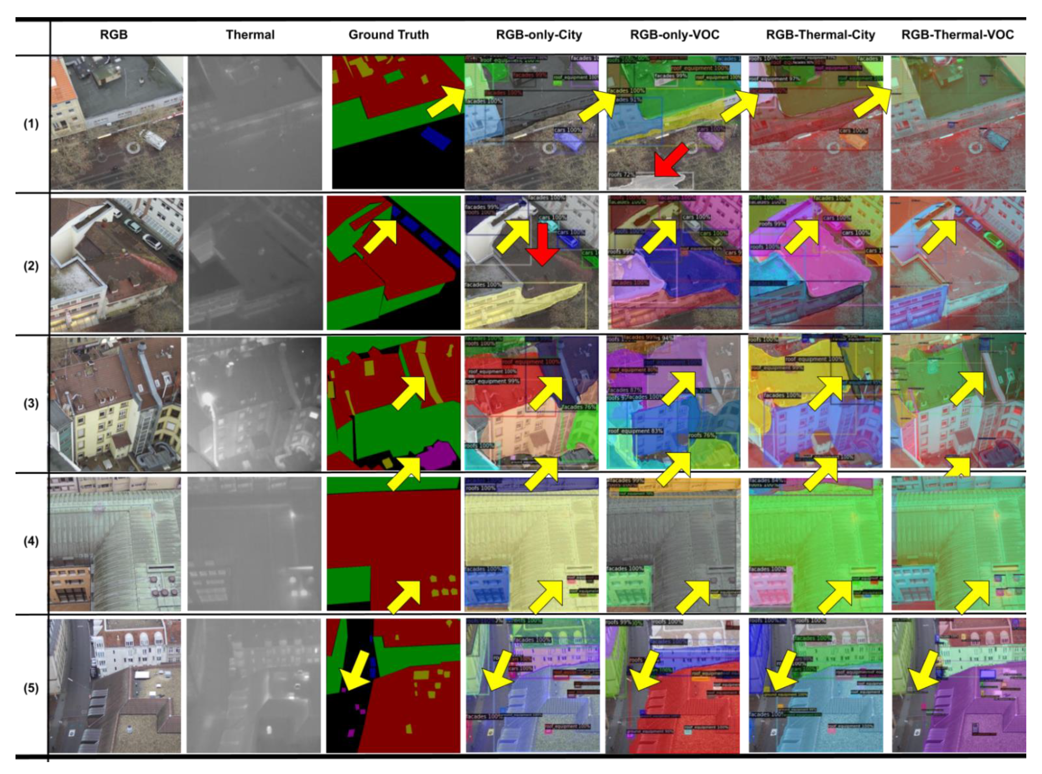
4.2. Evaluation of PSPNet and DeepLab v3+

In this section, we used the evaluation metrics—including precision, recall, IoU, accuracy, and F1 scores—to evaluate the performance of the implemented and trained PSPNet and DeepLab v3+ algorithms. We selected and calculated the average evaluation values from the last 20 epochs (1/10 of total epochs). The performances are summarized in

Table 3. Performance evaluation of PSPNet and DeepLab v3+.

Index	Algorithms	ACC	F1	IoU	Precision	Recall	Memory Per Iteration	Training Time Per Iteration
1	RGB-only- City-DeepLabv3+	0.91621	0.79454	0.68392	0.86021	0.75690	1400–1500 MB	0.2–0.3 s
2	RGB-only- City-PSPNet	0.91712	0.79213	0.68199	0.85542	0.75468
3	RGB-only- VOC-DeepLabv3+	0.91686	0.79846	0.68930	0.85561	0.76388
4	RGB-only- VOC-PSPNet	0.91759	0.79232	0.68347	0.85904	0.75432
5	RGB-Thermal- City-DeepLabv3+	0.91546	0.79576	0.68426	0.84683	0.76195
6	RGB-Thermal- City-PSPNet	0.91556	0.78685	0.67646	0.84792	0.75238
7	RGB-Thermal- VOC-DeepLabv3+	0.91638	0.79561	0.68491	0.85775	0.75978
8	RGB-Thermal- VOC-PSPNet	0.91567	0.78870	0.67818	0.85354	0.75136

and

Table 4. Performance evaluation of PSPNet and DeepLab v3+ in terms of IoU.

Index	Algorithms	IoU.Background	IoU.Cars	IoU.Facades	IoU.Ground_Equipment	IoU.Roof_Equipment	IoU.Roofs
1	RGB-only- City-DeepLabv3+	0.80200	0.73955	0.79259	0.32389	0.54672	0.89874
2	RGB-only- City-PSPNet	0.80532	0.74463	0.79551	0.31752	0.5294	0.89961
3	RGB-only- VOC-DeepLabv3+	0.80249	0.75421	0.79487	0.32512	0.56011	0.89900
4	RGB-only- VOC-PSPNet	0.80674	0.75462	0.79513	0.30555	0.53918	0.89961
5	RGB-Thermal- City-DeepLabv3+	0.79940	0.73289	0.79512	0.33899	0.54223	0.89686
6	RGB-Thermal- City-PSPNet	0.80279	0.74061	0.79102	0.29864	0.52828	0.89738
7	RGB-Thermal- VOC-DeepLabv3+	0.80260	0.73676	0.79529	0.33040	0.54663	0.89781
8	RGB-Thermal- VOC-PSPNet	0.80201	0.74216	0.79298	0.30767	0.52699	0.89723

. First, the metrics in Table 3 display evaluation over all categories, while the metrics in Table 4 reflect the IoU of different categories. Second, the headers in Table 3 and Table 4 represent the evaluation metrics, and each row with its index number represents different experiments that tested distinct algorithms using various pretrained models and training datasets. Third, in this section, the algorithms include DeepLab v3+ and PSPNet. The pretrained models that provide initial parameters use the Cityscapes and VOC open-source datasets. Fourth, the training datasets consist of two versions: one only has RGB images, while the other fuses RGB and thermal images. Therefore, the experiments presented in Table 3 are the different combinations of algorithms, datasets, and pretrained models. For example, “RGB-only-City-DeepLabv3+” represents the DeepLab v3+ algorithm experiment with the training dataset that only had RGB images, and the initial DeepLab v3+ parameters were set by using the Cityscapes pretrained model. Finally, the different colors represent the values, and darker colors represent a greater value, which means a better performance.

According to Table 3, we can analyze the performance based on the color patterns. First, DeepLab v3+ outperforms PSPNet in many evaluation metrics, as shown in the comparison between rows 1 and 2, rows 3 and 4, rows 5 and 6, and rows 7 and 8. Second, as for the initial parameters provided by pretrained models, VOC outperforms Cityscape in most cases, as shown in the comparison between rows 3–4 and 1–2, and between the rows 7–8 and 5–6. Third, fusing thermal channels does not significantly outperform datasets with only RGB images when evaluating all categories. Therefore, we need to respectively evaluate the performance in terms of their categories.

Since IoU is one of the most “perfect” and commonly used performance evaluation metrics, in Table 4, we summarize the IoU metrics in terms of categories, in which the background represents a category where the predicted segmentation does not belong to any of the analyzed categories. First, in Table 4, the color patterns show that adding thermal channels generally improves the performance of segmenting roof equipment and ground equipment. Second, PSPNet outperforms DeepLab v3+ in some categories, despite its overall poor performance—for example, in Table 4, the comparison between rows 1 and 2 and rows 3 and 4. Third, the initial parameters provided by the pretrained model VOC constantly outperform those of Cityscape in many cases.

4.3. Evaluation of Mask R-CNN

A difference exists between instance and semantic segmentation when evaluating prediction results. Semantic segmentation is a pixel-wise method, which means that each pixel in an image only has one label. For example, if a pixel is predicted for the roof equipment, it does not belong to the roof category. On the other hand, instance segmentation is an object-wise method, which means that each pixel can belong to multiple categories; for example, a pixel can be classified into both the roof and roof equipment categories. Due to the multiple predictions for one class, it is sometimes difficult to match the prediction with the ground truth for instance segmentation. Therefore, we need to configure an IoU threshold to check the match between the prediction and the ground truth. The IoU calculation is introduced in (3).

In this section, Mask R-CNN, as an instance segmentation algorithm, needs different evaluation metrics from those in Section 4.2.

Table 5. Performance evaluation of Mask R-CNN.

Index	Algorithms	Precision Value	Precision -Cars	Precision -Facades	Precision -Ground_ Equipment	Precision -Roof_ Equipment	Precision -Roofs	Precision @ IoU ≥ 0.5	Precision @ IoU ≥ 0.75	Precision-Large	Precision-Medium	Precision-Small
1	RGB_ only_ VOC	30.50027	48.50009	39.40096	7.894894	18.51801	38.18739	53.82021	31.2914	25.17297	30.15385	10.09727
2	RGB_ only_ City	36.40356	56.87393	39.8599	13.93462	25.40921	44.08705	61.05142	37.09566	30.71153	35.43907	18.89682
3	RGB_ Thermal_VOC	34.67095	53.46492	38.34726	13.29906	23.57708	44.66644	59.18085	35.19486	32.31295	32.6255	13.10268
4	RGB_ Thermal_City	39.69939	59.65007	38.87487	18.22493	26.52003	49.22706	63.64552	41.1819	38.88473	39.07861	17.92202
Memory per iteration							4500–4600 MB
Training time per iteration							0.5–0.6 s

presents Mask R-CNN’s performance. First, we needed to determine which predicted bounding boxes corresponded to correct predictions, so we used IoU (3) to measure the predicted and ground-truth bounding boxes. For a given IoU threshold, predicted bounding boxes that have an IoU with an annotated object class’ bounding box above the threshold are considered true positives. However, other annotated classes that do not satisfy this requirement are considered false negatives. As (2) shows, we calculated the precision for predicted bounding boxes and segmentations that met the IoU threshold requirement. Table 5 shows the precision values in various situations, such as the precision values for an individual class, an IoU threshold greater than 0.5, an IoU threshold greater than 0.75, or an object class with small, medium, and large areas. Areas of small, medium, and large correspond to objects of areas less than 322, between 322 and 962, and greater than 962 pixels, respectively.

Color illustrates the numbers—the higher the number, the darker the color. First, as shown in Table 5, adding thermal information allows for improvement of segmentation performance. Rows 3 and 4 are noticeably darker than rows 1 and 2. Second, compared to other categories, adding thermal information does not improve the segmentation performance on the facade category. Third, the pretrained parameters using Cityscape datasets outperform the pretrained parameters using VOC datasets. This observation is contrary to the semantic segmentation in Section 4.2. Finally, as for the computational complexity, memory and training time per iteration are both smaller in the semantic segmentation case, as shown in Table 3 and Table 4.

4.4. Discussion

To analyze the algorithms’ performance, we show five successful and failed cases in Figure 5 and Figure 6. In the first case, these segmentation algorithms implemented on different datasets have good performances; however, none of these semantic segmentation algorithms can detect the roof equipment that is indicated by the left arrow in Figure 5; as shown in Figure 6, only Mask R-CNN using RGB-fused thermal datasets can detect that roof equipment object. Another observation in case one is that the facade pixels surrounded by roof pixels can barely be detected by PSPNet, as shown by the right arrow in Figure 5; conversely, as shown in Figure 6, it is not difficult for Mask R-CNN to detect that facade object. One mistake made by Mask R-CNN that should be pointed out is that the algorithm incorrectly detects the road as belonging to the roof category in the “RGB-only-VOC” column, as shown by the red arrow in Figure 6. In the second case, as shown by the arrows in Figure 5, it is hard for the roof pixels surrounded by facade pixels to be detected. However, adding a thermal channel slightly improves the performance, as shown by the arrows. In Figure 6, this is not a problem for Mask R-CNN; however, Mask R-CNN failed to detect a large area of the roof category in the “RGB-only-City” column, as shown by the red arrow. In case three, as shown by the upper arrow, none of the semantic segmentation algorithms can detect this roof equipment in Figure 5, but “RGB-Thermal-City” detects this roof equipment in Figure 6. As shown by the lower arrow, none of the semantic segmentation algorithms can detect this ground equipment—most of them predict that area as belonging to the roof category, while PSPNet and Mask R-CNN predict that area as belonging to the roof equipment category. The fourth case illustrates that adding a thermal channel can help to detect and separate roof equipment. As shown in Figure 5, “RGB-only-City-PSPNet” cannot even predict any roof equipment objects. With the assistance of a thermal channel, “RGB-Thermal-City-PSPNet” can fully detect all roof equipment objects. Mask R-CNN performs well in this case, but not in the “RGB-only-VOC” column in Figure 6. The fifth case illustrates that adding a thermal channel allows for the improvement of ground equipment segmentation. This can be observed in both semantic and instance segmentation.

In summary, first, adding a thermal channel has a better effect on improving the segmentation of roof and ground equipment than improving other categories in most cases. Second, Mask R-CNN is good at differentiating small objects, such as equipment and cars, and this may be a result of its neural network structure. As mentioned in the methodology, Mask R-CNN first proposes ROIs, and then predicts the semantic information on them. Large objects, such as roofs and facades, occupy a large portion of the whole image, so Mask R-CNN may not detect salient features from these objects. In contrast, for the small objects—such as equipment and cars—because Mask R-CNN can see their whole shapes, it can easily detect them. For example, in the second case in Figure 6, there are four cars in the ground truth, but Mask R-CNN can only detect three of them. On the other hand, semantic segmentation can detect all four cars. Third, with the assistance of thermal information, equipment segmentation performance is improved, but both semantic and instance segmentation can still confuse roof equipment and ground equipment; since only 2D information is provided, the algorithms cannot distinguish between equipment on the roofs and on the ground. This could be solved by implementing depth/height information into the analysis [50].

5. Conclusions and Future Studies

Several important conclusions can be drawn from this study. First, adding thermal channels allows for improving the semantic and instance segmentation performance. Second, the thermal channel performs differently for different types of classes; its performance also differs when using different algorithms. Third, Mask R-CNN, as an instance segmentation algorithm, can individually predict small objects such as roof equipment and ground equipment; it does not predict the same object as a whole group of pixels in a picture, as is the case in semantic segmentation algorithms. The benefit of using the instance segmentation algorithm is that it allows researchers to distinguish different roof and facade objects, which further allows researchers to index individual thermal bridges and heating losses from building envelopes more conveniently. Fourth, in terms of time and memory complexity, both PSPNet and DeepLab v3+ outperform Mask R-CNN, since these two semantic segmentation approaches do not need to propose ROIs, and their networks are simpler than Mask R-CNN’s network.

There are some drawbacks to this study; for example, according to Table 2, the number of instances of roof equipment and ground equipment is smaller than other objects in our datasets. This imbalance might cause inaccuracy for segmenting roof equipment and ground equipment objects. In future research, we need to balance the ratio of different objects in the dataset. Second, despite the performance improvement by adding the thermal features to the networks, the main limitation of using thermal information is its reliability across different geographical locations with various climate zones, seasons, and weather conditions. Thus, the models trained in this study may have a poor performance on the data collected from a place with distinct weather conditions. This issue could be potentially addressed by enlarging the training datasets, since a more extensive dataset can include more cases to improve training performance. Although there are insufficient open-source data shared between civil engineering projects for energy audits using thermal images, object segmentation tasks need a large dataset to improve segmentation accuracy. Thus, we plan to use synthetic thermal imagery data to enlarge the database. The synthetic data can potentially be generated using our previous work on creating synthetic 3D environments and annotated aerial photogrammetry data [20,60].

Furthermore, after reviewing current open-source datasets, we did not find helpful outdoor scene datasets for building envelope energy audits in the field of civil engineering. As one of the conclusions drawn, our datasets contribute to the building science field by enabling researchers to easily distinguish roof and facade objects for energy audits. We plan to improve our studies in these fields. First, we plan to investigate the semantic segmentation using 3D models. As we have learned, although instance segmentation has enabled researchers to index objects, they still cannot relate heat loss to the location of a building. Directly segmenting objects from 3D models can provide an alternative approach. Additionally, 3D models provide depth information, with which roof equipment and ground equipment can be easily distinguished. Finally, as we only explored input fusion approaches in this study, we plan to implement other fusion approaches for segmentation.

References

1. Hou, Y.; Mayer, Z.; Li, Z.; Volk, R.; Soibelman, L. An Innovative Approach for Building Facade Component Segmentation on 3D Point Cloud Models Reconstructed by Aerial Images. In Proceedings of the 28th International Workshop on Intelligent Computing in Engineering, Berlin, Germany, 30 June–2 July 2021; pp. 1–10. [Google Scholar]
2. Lin, D.; Jarzabek-Rychard, M.; Schneider, D.; Maas, H.G. Thermal texture selection and correction for building facade inspection based on thermal radiant characteristics. Int. Arch. Photogramm. Remote Sens. Spat. Inf. Sci.-ISPRS Arch. 2018, 42, 585–591. [Google Scholar] [CrossRef] [Green Version]
3. Lin, D.; Jarzabek-rychard, M.; Tong, X.; Maas, H. Fusion of thermal imagery with point clouds for building façade thermal attribute mapping. ISPRS J. Photogramm. Remote Sens. 2019, 151, 162–175. [Google Scholar] [CrossRef]
4. Hou, Y.; Soibelman, L.; Volk, R.; Chen, M. Factors Affecting the Performance of 3D Thermal Mapping for Energy Audits in A District by Using Infrared Thermography (IRT) Mounted on Unmanned Aircraft Systems (UAS). In Proceedings of the 36th International Symposium on Automation and Robotics in Construction (ISARC), Banff, AB, Canada, 21–24 May 2019; pp. 266–273. [Google Scholar] [CrossRef]
5. Yao, X.; Wang, X.; Zhong, Y.; Liangpei, Z. Thermal Anomaly Detection based on Saliency Computation for Dristrict Heating System. 2016, pp. 681–684. Available online: http://ieeexplore.ieee.org/stamp/stamp.jsp?arnumber=7729171 (accessed on 24 October 2021).
6. Friman, O.; Follo, P.; Ahlberg, J.; Sjökvist, S. Methods for Large-Scale Monitoring of District Heating Systems Using Airborne Thermography Methods for Large-Scale Monitoring of District Heating Systems using Airborne Thermography. IEEE Trans. Geosci. Remote. Sens. 2014, 52, 5175–5182. [Google Scholar] [CrossRef] [Green Version]
7. Bauer, E.; Pavón, E.; Barreira, E.; de Castro, E.K. Analysis of building facade defects using infrared thermography: Laboratory studies. J. Build. Eng. 2016, 6, 93–104. [Google Scholar] [CrossRef]
8. He, K.; Gkioxari, G.; Dollár, P.; Girshick, R. Mask R-CNN. IEEE Trans. Pattern Anal. Mach. Intell. 2020, 42, 386–397. [Google Scholar] [CrossRef]
9. Wong, A.; Famuori, M.; Shafiee, M.J.; Li, F.; Chwyl, B.; Chung, J. YOLO Nano: A Highly Compact You Only Look Once Convolutional Neural Network for Object Detection. arXiv Prepr. 2019, arXiv:1910.01271, 1–5. [Google Scholar]
10. Chen, L.C.; Papandreou, G.; Kokkinos, I.; Murphy, K.; Yuille, A.L. DeepLab: Semantic Image Segmentation with Deep Convolutional Nets, Atrous Convolution, and Fully Connected CRFs. IEEE Trans. Pattern Anal. Mach. Intell. 2018, 40, 834–848. [Google Scholar] [CrossRef]
11. Spicer, R.; Mcalinden, R.; Conover, D. Producing Usable Simulation Terrain Data from UAS-Collected Imagery. In Proceedings of the 2016 Interservice/Industry Training Systems and Education Conference (I/ITSEC), Orlando, FL, USA, 4–7 December 2006; pp. 1–13. [Google Scholar]
12. Garcia-Garcia, A.; Orts-Escolano, S.; Oprea, S.; Villena-Martinez, V.; Garcia-Rodriguez, J. A Review on Deep Learning Techniques Applied to Semantic Segmentation. 2017, pp. 1–23. Available online: http://arxiv.org/abs/1704.06857 (accessed on 24 October 2021).
13. Park, S.; Lee, S. RDFNet: RGB-D Multi-level Residual Feature Fusion for Indoor Semantic Segmentation Ki-Sang Hong. In Proceedings of the IEEE International Conference on Computer Vision (ICCV), Cambridge, MA, USA, 20–23 June 2017; pp. 4980–4989. [Google Scholar]
14. Wang, J.; Wang, Z.; Tao, D.; See, S.; Wang, G. Learning common and specific features for RGB-D semantic segmentation with deconvolutional networks, Lecture Notes in Computer Science (including subseries Lecture Notes in Artificial Intelligence and Lecture Notes in Bioinformatics). In European Conference on Computer Vision; Springer: Berlin/Heidelberg, Germany, 2016; Volume 9909 LNCS, pp. 664–679. [Google Scholar] [CrossRef] [Green Version]
15. Berg, A.; Ahlberg, J. Classification of leakage detections acquired by airborne thermography of district heating networks. In Proceedings of the 2014 8th IAPR Workshop on Pattern Recognition in Remote Sensing. PRRS 2014, Stockholm, Sweden, 24 August 2014. [Google Scholar] [CrossRef] [Green Version]
16. Berg, A.; Ahlberg, J.; Felsberg, M. Enhanced analysis of thermographic images for monitoring of district heat pipe networks. Pattern Recognit. Lett. 2016, 83, 215–223. [Google Scholar] [CrossRef] [Green Version]
17. Cho, Y.K.; Ham, Y.; Golpavar-Fard, M. 3D as-is building energy modeling and diagnostics: A review of the state-of-the-art. Adv. Eng. Inform. 2015, 29, 184–195. [Google Scholar] [CrossRef]
18. Lucchi, E. Applications of the infrared thermography in the energy audit of buildings: A review. Renew. Sustain. Energy Rev. 2018, 82, 3077–3090. [Google Scholar] [CrossRef]
19. Maroy, K.; Carbonez, K.; Steeman, M.; van den Bossche, N. Assessing the thermal performance of insulating glass units with infrared thermography: Potential and limitations. Energy Build. 2017, 138, 175–192. [Google Scholar] [CrossRef]
20. Hou, Y.; Volk, R.; Soibelman, L. A Novel Building Temperature Simulation Approach Driven by Expanding Semantic Segmentation Training Datasets with Synthetic Aerial Thermal Images. Energies 2021, 14, 353. [Google Scholar] [CrossRef]
21. Nardi, I.; Lucchi, E.; de Rubeis, T.; Ambrosini, D. Quantification of heat energy losses through the building envelope: A state-of-the-art analysis with critical and comprehensive review on infrared thermography. Build. Environ. 2018, 146, 190–205. [Google Scholar] [CrossRef] [Green Version]
22. Barreira, E.; Almeida, R.M.S.F.; Moreira, M. An infrared thermography passive approach to assess the effect of leakage points in buildings. Energy Build. 2017, 140, 224–235. [Google Scholar] [CrossRef]
23. Balaras, C.A.; Argiriou, A.A. Infrared thermography for building diagnostics. Energy Build. 2002, 34, 171–183. [Google Scholar] [CrossRef]
24. Tejedor, B.; Casals, M.; Gangolells, M.; Roca, X. Quantitative internal infrared thermography for determining in-situ thermal behaviour of façades. Energy Build. 2017, 151, 187–197. [Google Scholar] [CrossRef]
25. Tejedor, B.; Casals, M.; Gangolells, M. Assessing the influence of operating conditions and thermophysical properties on the accuracy of in-situ measured U-values using quantitative internal infrared thermography. Energy Build. 2018, 171, 64–75. [Google Scholar] [CrossRef]
26. Bison, P.; Cadelano, G.; Grinzato, E. Thermographic Signal Reconstruction with periodic temperature variation applied to moisture classification. Quant. InfraRed Thermogr. J. 2011, 8, 221–238. [Google Scholar] [CrossRef] [Green Version]
27. Roselyn, J.P.; Uthra, R.A.; Raj, A.; Devaraj, D.; Bharadwaj, P.; Kaki, S.V.D.K. Development and implementation of novel sensor fusion algorithm for occupancy detection and automation in energy efficient buildings. Sustain. Cities Soc. 2019, 44, 85–98. [Google Scholar] [CrossRef]
28. Hou, Y.; Chen, M.; Volk, R.; Soibelman, L. Investigation on performance of RGB point cloud and thermal information data fusion for building thermal map modeling using aerial images under different experimental conditions. J. Build. Eng. 2021, 103380. [Google Scholar] [CrossRef]
29. Park, J.; Kim, P.; Cho, Y.K.; Kang, J. Framework for automated registration of UAV and UGV point clouds using local features in images. Autom. Constr. 2019, 98, 175–182. [Google Scholar] [CrossRef]
30. Balan, P.S.; Sunny, L.E. Survey on Feature Extraction Techniques in Image Processing. Int. J. Res. Appl. Sci. Eng. Technol. (IJRASET) 2018, 6, 217–222. [Google Scholar]
31. Hespanha, P.; Kriegman, D.J.; Belhumeur, P.N. Eigenfaces vs. Fisherfaces: Recognition Using Class Specific Linear Projection. IEEE Trans. pattern Anal. Mach. Intelligencevol. 1997, 19, 711–720. [Google Scholar]
32. Turk, M.A.; Pentland, A.P. Face Recognition Using Eigenfaces. In Proceedings of the 1991 IEEE Computer Society Conference on Computer Vision and Pattern Recognition, Maui, HI, USA, 3–6 June 1991; IEEE: Piscataway, NJ, USA, 1991; pp. 586–591. [Google Scholar]
33. Yambor, W.S.; Draper, B.A.; Beveridge, J.R. Analyzing PCA-based Face Recognition Algorithms: Eigenvector Selection and Distance Measures. In Empirical Evaluation Methods in Computer Vision; World Scientific: Singapore, 2000; pp. 1–14. [Google Scholar]
34. Martinez, A.M.; Kak, A.C. PCA versus LDA. IEEE Trans. Pattern Anal. Mach. Intell. 2001, 23, 228–233. [Google Scholar] [CrossRef] [Green Version]
35. Toygar, Ö.; Introduction, I. Face Recognition Using PCA, LDA AND ICA Approaches on Colored Images. IU-J. Electr. Electron. Eng. 2003, 3, 735–743. [Google Scholar]
36. Lowe, D.G. Object recognition from local scale-invariant features. In Proceedings of the Seventh IEEE International Conference on Computer Vision, Kerkyra, Greece, 20–27 September 1999; Volume 2, pp. 1150–1157. [Google Scholar] [CrossRef]
37. Ke, Y.; Sukthankar, R. PCA-SIFT: A more distinctive representation for local image descriptors, in null. In Proceedings of the 2004 IEEE Computer Society Conference on Computer Vision and Pattern Recognition, 2004. CVPR 2004, Washington, DC, USA, 27 June–2 July 2004; pp. 506–513. [Google Scholar]
38. Comon, P. Independent Component Analysis, A New Concept? Signal Process 1994, 287–314. [Google Scholar] [CrossRef]
39. Krizhevsky, A.; Sutskever, I.; Hinton, G.E. ImageNet Classification with Deep Convolutional Neural Networks. Commun. Assoc. Comput. Mach. 2017, 60, 84–90. [Google Scholar] [CrossRef]
40. Zeiler, M.D.; Fergus, R. Visualizing and understanding convolutional networks. In Proceedings of the in European Conference on Computer Vision, Zurich, Switzerland, 6–12 September 2014; pp. 818–833. [Google Scholar]
41. Jiang, M.X.; Deng, C.; Shan, J.S.; Wang, Y.Y.; Jia, Y.J.; Sun, X. Hierarchical multi-modal fusion FCN with attention model for RGB-D tracking. Inf. Fusion 2019, 50, 1–8. [Google Scholar] [CrossRef]
42. Caltagirone, L.; Bellone, M.; Svensson, L.; Wahde, M. LIDAR–camera fusion for road detection using fully convolutional neural networks. Robot. Auton. Syst. 2019, 111, 125–131. [Google Scholar] [CrossRef] [Green Version]
43. Zhao, H.; Shi, J.; Qi, X.; Wang, X.; Jia, J. Pyramid scene parsing network. In Proceedings of the 30th IEEE Conference on Computer Vision and Pattern Recognition, CVPR 2017, Honolulu, HI, USA, 21–26 July 2017; Volume 2017, pp. 6230–6239. [Google Scholar] [CrossRef] [Green Version]
44. Chen, L.C.; Zhu, Y.; Papandreou, G.; Schroff, F.; Adam, H. Encoder-decoder with atrous separable convolution for semantic image segmentation. Lect. Notes Comput. Sci. (Incl. Subser. Lect. Notes Artif. Intell. Lect. Notes Bioinform.) 2018, 11211 LNCS, 833–851. [Google Scholar] [CrossRef] [Green Version]
45. Paper with Code. 2021. Available online: https://paperswithcode.com/ (accessed on 27 May 2021).
46. Chen, L.-C.; Papandreou, G.; Schroff, F.; Adam, H. Rethinking Atrous Convolution for Semantic Image Segmentation. 2017. Available online: http://arxiv.org/abs/1706.05587 (accessed on 24 October 2021).
47. Aslam, Y.; Santhi, N.; Ramasamy, N.; Ramar, K. Localization and segmentation of metal cracks using deep learning. J. Ambient. Intell. Humaniz. Comput. 2020. [Google Scholar] [CrossRef]
48. Wu, T.; Tang, S.; Zhang, R.; Cao, J.; Zhang, Y. CGNet: A Light-Weight Context Guided Network for Semantic Segmentation. IEEE Trans. Image Process. 2021, 30, 1169–1179. [Google Scholar] [CrossRef] [PubMed]
49. Xiao, T.; Liu, Y.; Zhou, B.; Jiang, Y.; Sun, J. Unified Perceptual Parsing for Scene Understanding. Lect. Notes Comput. Sci. (Incl. Subser. Lect. Notes Artif. Intell. Lect. Notes Bioinform.) 2018, 11209 LNCS, 432–448. [Google Scholar] [CrossRef] [Green Version]
50. Mayer, Z.; Hou, Y.; Kahn, J.; Beiersdörfer, T.; Volk, R. Thermal Bridges on Building Rooftops—Hyperspectral (RGB + Thermal + Height) drone images of Karlsruhe, Germany, with thermal bridge annotations. Repos. KITopen 2021. [Google Scholar] [CrossRef]
51. Nawaz, M.; Yan, H. Saliency Detection using Deep Features and Affinity-based Robust Background Subtraction. IEEE Trans. Multimed. 2020. [Google Scholar] [CrossRef]
52. Chen, H.; Li, Y. Progressively Complementarity-Aware Fusion Network for RGB-D Salient Object Detection. In Proceedings of the in 2018 IEEE/CVF Conference on Computer Vision and Pattern Recognition, Salt Lake City, UT, USA, 18–23 June 2018; pp. 3051–3060. [Google Scholar] [CrossRef]
53. Chen, H.; Li, Y.; Su, D. Multi-modal fusion network with multi-scale multi-path and cross-modal interactions for RGB-D salient object detection. Pattern Recognit. 2019, 86, 376–385. [Google Scholar] [CrossRef]
54. Ren, J.; Gong, X.; Yu, L.; Zhou, W.; Yang, M.Y. Exploiting global priors for RGB-D saliency detection. In Proceedings of the IEEE Computer Society Conference on Computer Vision and Pattern Recognition Workshops, Boston, MA, USA, 7–12 June 2015; Volume 2015-Octob, pp. 25–32. [Google Scholar] [CrossRef]
55. Peng, H.; Li, B.; Xiong, W.; Hu, W.; Ji, R. RGBD salient object detection: A benchmark and algorithms. Lect. Notes Comput. Sci. (Incl. Subser. Lect. Notes Artif. Intell. Lect. Notes Bioinform.) 2014, 8691 LNCS, 92–109. [Google Scholar] [CrossRef]
56. Qu, L.; He, S.; Zhang, J.; Tian, J.; Tang, Y.; Yang, Q. RGBD Salient Object Detection via Deep Fusion. IEEE Trans. Image Process. 2017, 26, 2274–2285. [Google Scholar] [CrossRef]
57. Desingh, K.; K, M.K.; Rajan, D.; Jawahar, C. Depth really Matters: Improving Visual Salient Region Detection with Depth. In Proceedings of the BMVC, Nottingham, UK, 1–5 September 2014; pp. 1–11. [Google Scholar] [CrossRef] [Green Version]
58. Wang, N.; Gong, X. Adaptive fusion for rgb-d salient object detection. IEEE Access 2019, 7, 55277–55284. [Google Scholar] [CrossRef]
59. van der Ploeg, T.; Austin, P.C.; Steyerberg, E.W. Modern modelling techniques are data hungry: A simulation study for predicting dichotomous endpoints. BMC Med Res. Methodol. 2014, 14, 137. [Google Scholar] [CrossRef] [PubMed] [Green Version]
60. Chen, M.; Feng, A.; Mcalinden, R.; Soibelman, L. Generating Synthetic Photogrammetric Data for Training Deep Learning based 3D Point Cloud Segmentation Models. arXiv 2020, arXiv:2008.09647v120221, 1–12. [Google Scholar]
61. Chen, M.; Feng, A.; McCullough, K.; Prasad, P.B.; McAlinden, R.; Soibelman, L. 3D Photogrammetry Point Cloud Segmentation Using a Model Ensembling Framework. J. Comput. Civ. Eng. 2020, 34, 1–20. [Google Scholar] [CrossRef]
62. Chen, M.; Feng, A.; Mccullough, K.; Prasad, B.; Mcalinden, R.; Soibelman, L. Semantic Segmentation and Data Fusion of Microsoft Bing 3D Cities and Small UAV-based Photogrammetric Data. arXiv 2020, arXiv:2008.09648v120220, 1–12. [Google Scholar]
63. Hou, Y.; Volk, R.; Chen, M.; Soibelman, L. Fusing tie points’ RGB and thermal information for mapping large areas based on aerial images: A study of fusion performance under different flight configurations and experimental conditions. Autom. Constr. 2021, 124. [Google Scholar] [CrossRef]
64. Lagüela, S.; Armesto, J.; Arias, P.; Herráez, J. Automation of thermographic 3D modelling through image fusion and image matching techniques. Autom. Constr. 2012, 27, 24–31. [Google Scholar] [CrossRef]
65. Luo, C.; Sun, B.; Yang, K.; Lu, T.; Yeh, W.C. Thermal infrared and visible sequences fusion tracking based on a hybrid tracking framework with adaptive weighting scheme. Infrared Phys. Technol. 2019, 99, 265–276. [Google Scholar] [CrossRef]
66. Li, C.; Wu, X.; Zhao, N.; Cao, X.; Tang, J. Fusing two-stream convolutional neural networks for RGB-T object tracking. Neurocomputing 2018, 281, 78–85. [Google Scholar] [CrossRef]
67. Zhai, S.; Shao, P.; Liang, X.; Wang, X. Fast RGB-T Tracking via Cross-Modal Correlation Filters. Neurocomputing 2019, 334, 172–181. [Google Scholar] [CrossRef]
68. Jiang, J.; Jin, K.; Qi, M.; Wang, Q.; Wu, J.; Chen, C. A Cross-Modal Multi-granularity Attention Network for RGB-IR Person Re-identification. Neurocomputing 2020, 406, 59–67. [Google Scholar] [CrossRef]
69. Mayer, Z.; Hou, Y.; Kahn, J.; Volk, R.; Schultmann, F. AI-Based Thermal Bridge Detection of Building Rooftops on District Scale Using Aerial Images. 2021. Available online: https://publikationen.bibliothek.kit.edu/1000136256/123066859 (accessed on 24 October 2021).
Figure 1. Image data fusion categories.
Remotesensing 13 04357 g001
Figure 2. Illustration of the fusion approach on PSPNet.
Remotesensing 13 04357 g002
Figure 3. Illustration of the fusion approach on DeepLab v3+.
Remotesensing 13 04357 g003
Figure 4. The fusion approach on Mask R-CNN.
Remotesensing 13 04357 g004
Figure 5. Semantic segmentation detected by algorithms.
Remotesensing 13 04357 g005
Figure 6. Instance segmentation by Mask R-CNN.
Remotesensing 13 04357 g006