Article

Multidirectional Shift Rasterization (MDSR) Algorithm for Effective Identification of Ground in Dense Point Clouds

Department of Special Geodesy, Faculty of Civil Engineering, Czech Technical University in Prague, Thákurova 7, 166 29 Prague, Czech Republic
*
Author to whom correspondence should be addressed.
Remote Sens. 2022, 14(19), 4916; https://doi.org/10.3390/rs14194916
Submission received: 24 August 2022 / Revised: 20 September 2022 / Accepted: 28 September 2022 / Published: 1 October 2022
(This article belongs to the Special Issue UAVs for Civil Engineering Applications)

Abstract

:
With the ever-increasing popularity of unmanned aerial vehicles and other platforms providing dense point clouds, filters for the identification of ground points in such dense clouds are needed. Many filters have been proposed and are widely used, usually based on the determination of an original surface approximation and subsequent identification of points within a predefined distance from such surface. We presented a new filter, the multidirectional shift rasterization (MDSR) algorithm, which is based on a different principle, i.e., on the identification of just the lowest points in individual grid cells, shifting the grid along both the planar axis and subsequent tilting of the entire grid. The principle was presented in detail and both visually and numerically compared with other commonly used ground filters (PMF, SMRF, CSF, and ATIN) on three sites with different ruggedness and vegetation density. Visually, the MDSR filter showed the smoothest and thinnest ground profiles, with the ATIN the only filter comparably performing. The same was confirmed when comparing the ground filtered by other filters with the MDSR-based surface. The goodness of fit with the original cloud is demonstrated by the root mean square deviations (RMSDs) of the points from the original cloud found below the MDSR-generated surface (ranging, depending on the site, between 0.6 and 2.5 cm). In conclusion, this paper introduced a newly developed MDSR filter that outstandingly performed at all sites, identifying the ground points with great accuracy while filtering out the maximum of vegetation and above-ground points and outperforming the aforementioned widely used filters. The filter dilutes the cloud somewhat; in such dense point clouds, however, this can be perceived as a benefit rather than as a disadvantage.

1. Introduction

Advances in the current measurement techniques have made it possible to routinely use advanced methods of bulk data collection, which found application not only in the technical and engineering fields. Acquisition of such data is possible using 3D scanners (lidars) or photogrammetric systems (usually based on the Structure from Motion method), mounted on a static platform [1], standard ground- or airborne platforms such as a UAV [2,3,4], or even an airship [5]. Such measurement systems result in point clouds of typically hundreds of millions to billions of points. Such large-scale data cannot be processed without at least semi-automated tools. Since at least some parts of the area of interest are massively oversampled, the initial processing phase usually involves dilution to the necessary (while usable) density, which is followed by the extraction of data needed for further processing. These activities typically include vegetation removal and, thus, extraction of points characterizing the objects of interest—be it the terrain, building structures, or anything else.
Such approaches to capturing the reality are being employed in many fields, from reality modeling for the identification of historical monuments [6], infrastructure mapping [7], mapping of open-pit mines [8], monitoring of changes during mining [9], coastline mapping [10], intertidal reef analysis [11], measurements for the purposes of building reconstruction [12], earthworks volume calculations [13], archaeological documentation [14], etc. Often, the data are processed to produce a general [15] or specialized [16] digital terrain model (DTM).

Current Ground Filtering Approaches

Vegetation removal or, more generally, identification of cloud points representing the terrain (ground) is a specific activity for which a considerable number of filters (algorithms and their implementations in software) have been developed. They can be classified into slope-based, interpolation-based, morphology-based, segmentation-based, statistics-based, and hybrid filters; machine learning; and other unclassified filters.
Slope-based filters work with the assumption that the terrain does not abruptly change; these methods determine the slopes in the vicinity of a point and compare the results with a maximum preset slope. These methods work fine in a flat terrain, but they are less effective in a rugged or forested landscape (e.g., [17,18,19]). Interpolation-based filters first select the “seed” ground points from the point cloud using a window size slightly exceeding the size of the biggest object in the area. Then, an approximation of the surface among such points is created and, using a threshold comparing the distance of the remaining points in the cloud from this surface, additional points are added (densify the cloud) (e.g., [20,21,22]). Morphology-based filters are based on the set theory and use operator definition (opening, closing, dilation, and erosion). Mostly, they compare the heights of the neighboring points, working with acceptable elevation differences depending on the horizontal distances of the points. Filtering quality depends on the filter cell size; to improve the filtering quality, morphological filters with gradually increasing cell size and threshold have been designed [23,24,25].
Segmentation-based filters divide the point cloud into segments, and each segment is labeled as either terrain or object; success depends on the quality of the segmentation. They work with point height, intensity, height difference, or geometric attributes (area, perimeter) [26,27,28,29]. Statistic-based filters are based on the fact that terrain points have a normal distribution in terms of height in a certain window, but an object or vegetation points violate this distribution. Based on this assumption, skewness and kurtosis parameters are calculated and used to judge whether a point is on the terrain or on an object [30,31]. These are methods in which no threshold is specified; for example, the method proposed by Bartels (skewness balancing [30]) takes into account the skewness value of the surrounding point cloud and deletes the highest point from the cloud if the skewness is greater than 0. The remaining group of unclassified filters can include, for example, a hybrid filter [32], cloth simulation filter [33], multiclass classification filter using a convolutional network [34,35], or a combination of a cloth simulation filter with progressive TIN densification [36]. Algorithms based on deep learning (neural networks) have also been investigated (e.g., [37,38,39,40,41,42]), but these need to be trained on specific data and are, therefore, probably not yet widely used.
As none of these approaches is universally applicable, the evaluation of the suitability of individual filters for specific purposes has recently been the subject of many scientific papers [42,43] and so has their sensitivity analysis [44].
Most known filtering techniques have been primarily developed for point clouds derived from airborne laser scanning (ALS), the nature of which is significantly different from the data acquired by systems mounted on small aerial vehicles (UAVs) and mobile or static ground platforms (regardless of whether they were mounted with laser scanners or collect imagery for the photogrammetric derivation of the cloud). The latter types of scanning systems typically provide high coverage density and extremely detailed and dense point clouds. Such data have been, in the past, typically predominantly used for relatively flat areas covered with buildings or vegetation. At present, remote sensing is increasingly used for measurements of relatively small areas with rugged rocks, quarries, or similar objects where vegetation removal is highly complicated even for a human operator. Thus, special filters and algorithms that go beyond the “standard” techniques and are capable of utilizing the dense clouds provided, for example, by UAV systems are being developed even for such specific situations [45,46,47].
Based on the above, it can be concluded that the general widely available ground filtering approaches are not suitable for many engineering applications, especially where rugged areas of smaller extent are concerned. Therefore, in this paper, we presented a newly developed filtering algorithm particularly designed for dense point clouds originating from UAV photogrammetry, UAV lidar, or terrestrial laser scanning (with typical densities of hundreds to thousands of points per square meter) in nature-close environments—the MDSR (multidirectional shift rasterization). This algorithm allows the acquisition of a terrain point cloud appropriately describing even the most rugged areas, which does not suffer from problems and artifacts typically found in geometric filters. In this algorithm, the terrain points are individually selected from the cloud as the lowest points of cells of a square grid, which is being gradually shifted in small steps and tilted about all three coordinate axes. In this paper, we aimed to (i) present the principle of the novel filtering algorithm, (ii) test its performance on three areas differing in the degree of ruggedness and vegetation cover, and (iii) compare its performance with that of selected widely used filters.

2. Materials and Methods

The proposed algorithm differs from the commonly used ones mainly in that it assumes a massive number of redundant points—a situation common in, for example, terrestrial, mobile, or UAV scanning, i.e., scanning with high detail. This assumption contrasts with the assumptions used in the majority of current algorithms (which were created for point clouds acquired by ALS). The algorithm does not aim to select all ground points existing in the point cloud, but rather it aims to identify a sufficient number of such points for accurate characterization of the course of the terrain with emphasis on the reliability of those points that were identified as the terrain.

2.1. Algorithm Description

The basic idea of the algorithm is that the lowest point from a certain area is likely to be a terrain point (or, to be more general, a point of the surface of interest covered by vegetation). Obviously, if such an area is square, this is similar to rasterization (but in rasterization, the lowest point detected in the cell is typically not left in its original location but used as a proxy for the whole square and cell and placed in its center). Without any doubt, the likelihood of the lowest point being a ground point increases with the increasing cell size. On the other hand, however, the larger the selected cell, the fewer the points left to characterize the terrain. The basic premise for the choice of the cell size is that it must be larger than the largest object that may lie on the terrain (i.e., a hole in the terrain data caused, for example, by occlusion by vegetation under which there is no point on the terrain, a building, etc.). In the real world, such a cell must necessarily cover an area of at least several meters. Thus, if the point cloud is processed by its division into square cells of sufficient size (in the horizontal plane), the lowest point in each of these cells is very likely to represent the terrain; the number of such points will, however, be very small, and many characteristic points of the terrain (e.g., the highest points of a ridge or pile) will be missing.
The presented method uses two techniques for point cloud densification and capturing the ground points even in the maxima (i.e., points with the highest ground elevation):
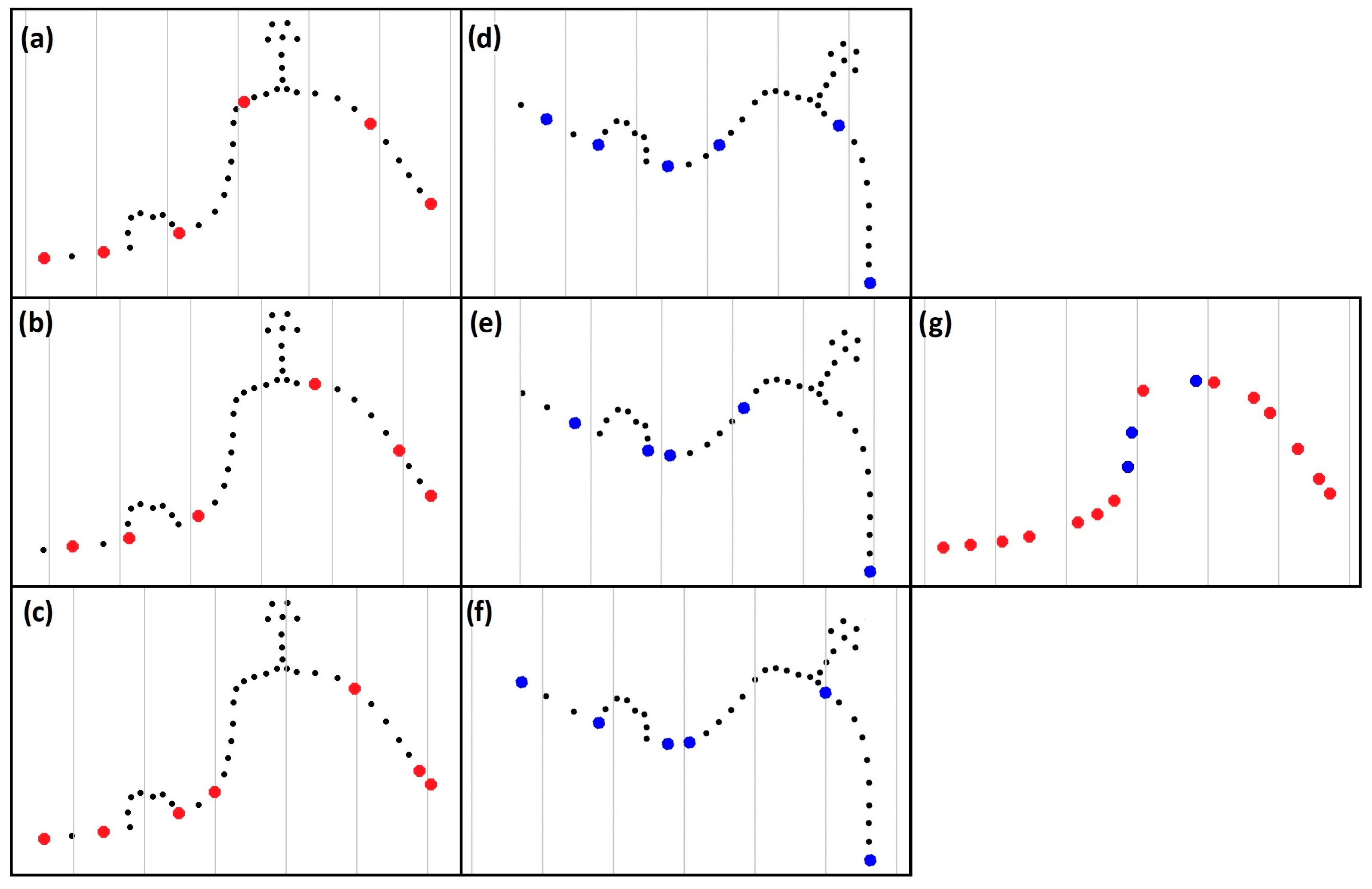
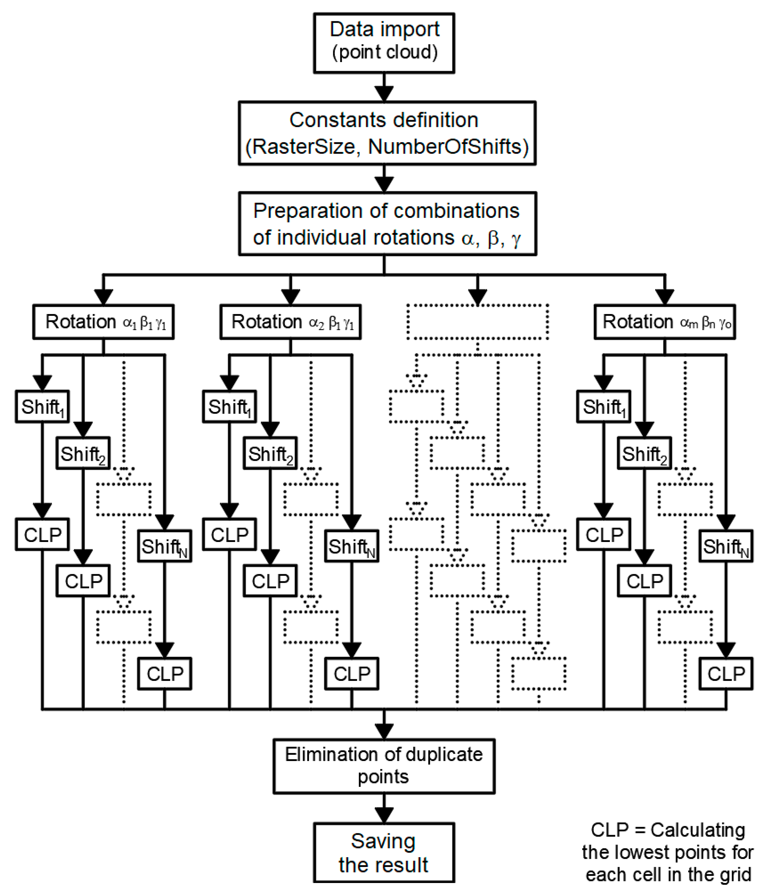
  • Moving the raster as a whole (i.e., shifting the cells in which the lowest point is identified) in steps much smaller than the cell size in both horizontal axes (X, Y);
  • Tilting (or, rather, rotation) of the raster around all 3 axes (X, Y, Z) changes the perspective for the evaluation of the elevations of individual points in the given projection. After such tilting, the raster is again gradually shifted as in the previous step, and points with the lowest elevation in each cell after each displacement are selected.
Figure 1 shows the basic ideas of the algorithm—the idea of shifting and rotating the grid. The figure shows only a cross-section; note, however, that the algorithm itself works in 3D, and, thus, if the cell size is large enough, the algorithm is able to bypass areas that are completely free of ground points (e.g., under a large tree; in such a case, the ground on the edge of the cell is selected, and, in the area without ground points, none are falsely selected). First, the cloud is divided into cells using a preset cell size (Figure 1, gray lines), and the lowest point within each cell is detected (Figure 1a, red dots). Subsequently, the grid moves (is shifted) by a preset distance and determines the lowest points in the cells that are newly created in this way, which densifies the cloud (Figure 1b,c). After that, the true innovation of this algorithm is applied—the point cloud is rotated, and the new projection of the grid on the terrain is used to detect the lowest points in thus newly created cells (Figure 1d, blue dots). Then, the grid is again shifted multiple times, and the lowest points after each such shift are determined to further densify the cloud (Figure 1e,f). Figure 1g shows the filtering result.
The algorithm in pseudocode is shown in Appendix A and the flowchart in Appendix B. The algorithm is designed to assign each point into a grid cell; if the assigned point is the lowest one in the cell at the time, it is recorded and the previous lowest point in the cell is deleted. In this way, all points are assigned and processed during a single pass for one position (shift and tilt) of the raster, which greatly reduces the computational demand compared with a situation in which all points within a cell would be first identified and the lowest of them subsequently selected. The algorithm is also suitable for easy parallelization; in our tests, 12 processors were simultaneously used.
The computational complexity, therefore, linearly increases with the number of cloud points and quadratically with the number of grid shifts, and, of course, it also increases with the increasing number of preset cloud rotations. The size of the grid (cell) determines the size of the objects that the method is able to bypass and, together with the grid shift size, also the detail of the resulting cloud.
It must be mentioned that if the edge of the cloud contains above-ground points, this thin margin will not be automatically corrected due to the oblique evaluation of the cloud, and it must be removed during further processing (manually or simply by cropping the entire filtered point cloud, which is preferable).

2.2. Illustration of the Algorithm Principle

The performance of the algorithm will be demonstrated on a simple example of data-capturing a rugged and heavily forested hill. The point cloud covering an area of 16,700 m2 was scanned by a UAV-lidar system UAV-DJI L1 (further information can be found in Appendix C); after dilution to a 0.07 m minimum distance between points, it contains 2,995,078 points. The site can be described as a ridge on a flat area (Figure 2), and, besides ruggedness, the data are characterized also by large holes in the terrain data caused by vegetation cover and a small stream running through the area (water absorbs the lidar beam).
Figure 3a shows a ground point cloud resulting from the basic rasterization and calculation of the lowest point in each cell of a 10 × 10 m grid (without any shifts and tilts).
As the area size is approximately 140 m × 130 m, the number of ground points will be very small if a 10 × 10 m cell is used. Given the cell size, these points are very likely to be indeed on the ground (and not on vegetation), but in terms of describing the landform, their density is certainly insufficient. Higher densities would be achievable by reducing the cell size, but in such a case, the cell would be likely, in many cases, smaller than the areas without ground data and filtering would be ineffective, identifying vegetation as ground points. Shifting the entire raster can lead to the potential identification of additional ground points. Figure 3b presents the situation after calculations using 5 × 5 displacements in the XxY direction (the grid was, therefore, shifted 5 times by 1/5 of the cell size in each direction). Here, we can observe the desired densification, but the terrain points on the vertices (or on the ridge as here) cannot be, on principle, correctly identified—in the vicinity of the ridge, any 10 × 10 m cell is bound to contain points with elevations lower than the ridge. This problem can be solved by changing the direction of the terrain view, i.e., by rotating the data (see Figure 3c–e—showing data filtered using individual rotations). Rotation also changes the projection of the cell on the terrain and, thus, changes the effective grid size, which also densifies the resulting cloud. Rotations should always be selected in a way corresponding to the estimated slopes of the surface (see below in the Methods). Figure 3f shows the filtering result of the combined data from 18 rotations (a combination of −50 gon, 0 gon, and +50 gon for rotations about the X- and Y-axes; 0 and 50 gon about the Z-axis), each of which was analyzed using 5 × 5 raster positions. Of the original approximately 3 million points, 29,000 remain, with an average density of 1.5 points/m2.
Figure 3 also demonstrates the presence of gaps in the data; this is most obvious along the ridge (e.g., Figure 3b,e). This gap position changes with individual rotations according to the apparent positions of the ridge relative to the remaining points from the virtual bird’s eye view. It is worth noting that the grid shift was also used as a part of the algorithm in [48], but without tilt (rotation), it is not possible to successfully filter areas close to the horizontal and especially the tops (ridges) of landforms or overhangs. The result of filtering without using rotation can be seen in Figure 3b with the already described gaps.

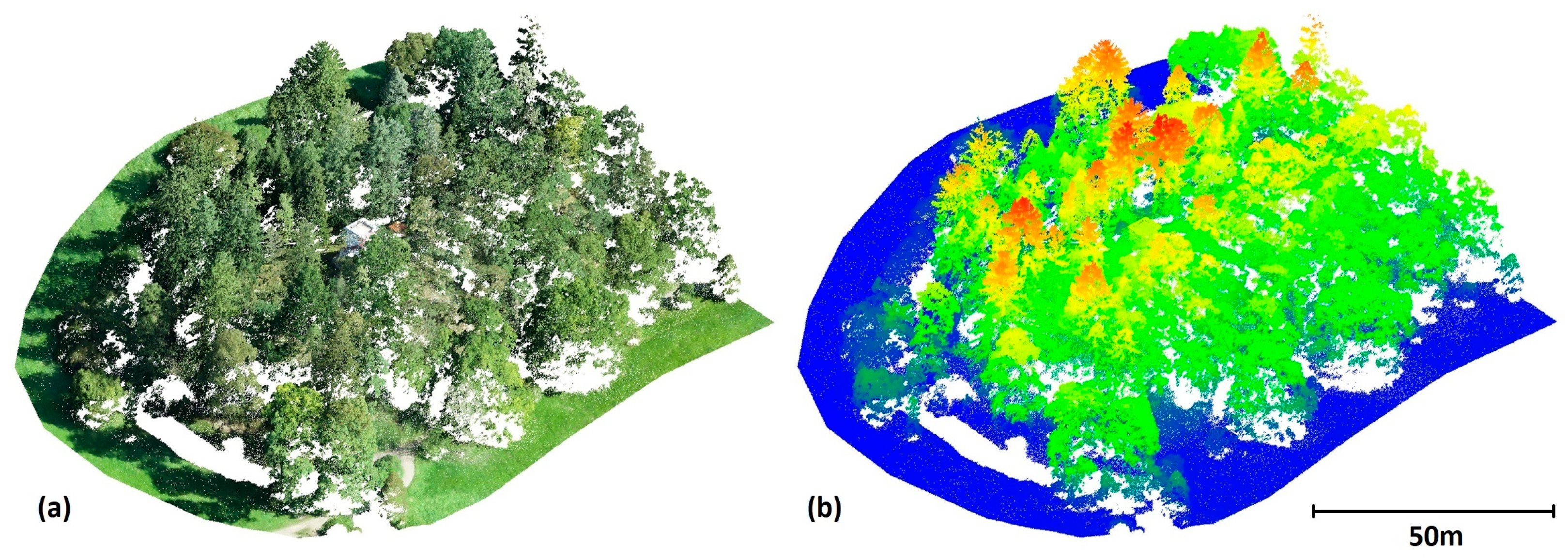
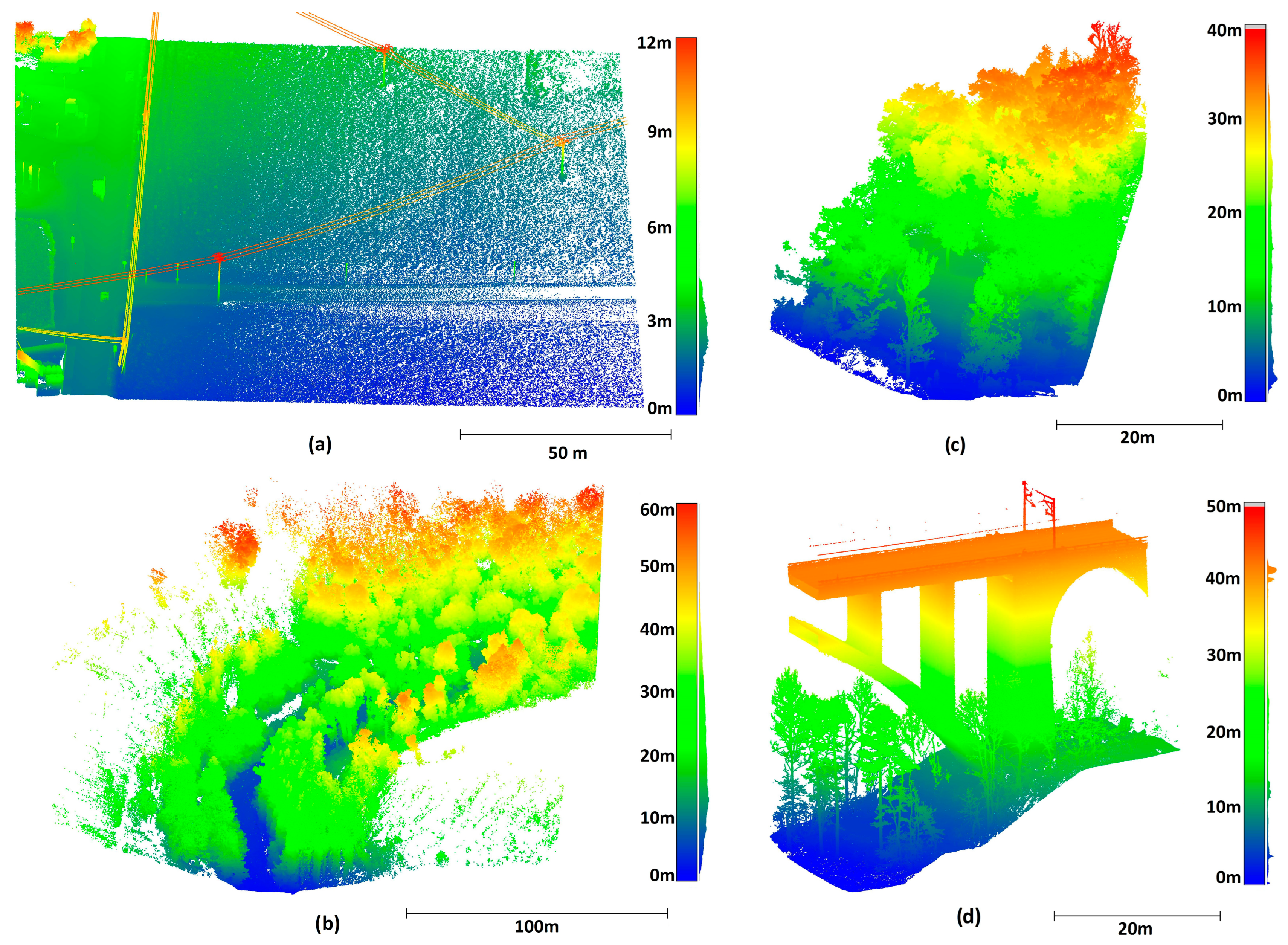
2.3. Data for Testing

The algorithm has been tested on point clouds acquired by mobile and terrestrial scanning systems. We present the results from terrains of varying complexity (different from the illustration dataset), from a virtually flat area through an extremely rugged and sloping rock face to a quarry area with a densely forested part of the surface, causing large gaps in terrain points. Lastly, as an example of an area with tall anthropomorphic objects, filtering of a rugged terrain with vegetation and bridge pillars is presented.
Site 1 (Figure 4a)—a virtually flat terrain with low vegetation; an area of 20,000 m2; diluted to 1,408,072 points with a minimum distance between neighboring points of 0.07 m; acquired using a Leica Pegasus mobile scanner mounted on a car (further information can be found in Appendix C). This dataset was selected as a basic one because it can be assumed that virtually any filter should be able to satisfactorily deal with its filtering.
Site 2 (Figure 4b)—a rural road surrounded by forest on steep slopes; a relatively rugged area of approximately 25,000 m2; 10,016,451 points; diluted to 0.07 m; acquired with a Leica Pegasus mobile scanner mounted on a car (further information can be found in Appendix C).
Site 3 (Figure 4c)—a virtually vertical cliff covered with vegetation, nets, and structures; an area of approximately 1240 m2; diluted to 0.05 m resolution; 2,785,912 points in total; acquired with a Trimble X7 terrestrial scanner (further information can be found in Appendix C). The data from this site contain high- as well as medium- and low-dense vegetation.
Site 4 (Figure 4d)—an area of approximately 1207 m2 with rugged terrain, low and tall vegetation, and tall bridge pillars combined with a curved bridge construction; diluted to a resolution of 0.07 m; 830,836 points in total; acquired by the combination of a terrestrial 3D scanner Leica P40 (mainly the construction) and UAV photogrammetry using a DJI Phantom 4 RTK (more information can be found in Appendix C).

2.4. Data Processing and Evaluation

The filter presented in this paper was programmed in the Scilab environment interpreted language (www.scilab.org (accessed on 6 May 2022), open-source software for numerical computation; version 6.1.1 was used). Since the latest versions of the environment do not allow parallel executions, the task was pre-divided into the required number of X parts (usually 12 on a 16-processor system) to speed up the computation.
As the data differ in character, various settings were used (detailed in Table 1). Partial rotations about individual axes were used in all combinations. As mentioned above, the estimated slopes of the terrain serve as a basis for the selection of the rotation angles—the angles of rotation should (i) roughly correspond to and (ii) slightly exceed the angles between all normals of the surface and the vertical direction (see the high number of angles needed for site 3 with extreme ruggedness). Note that if the steps are fine in one or two directions, the step in the remaining direction(s) can be somewhat greater as the combination of all rotations already ascertains sufficient detail.
As the dataset for site 3 is highly rugged and the surface is very steep, the range of rotations about the X-axis differs from those in other datasets. In site 4, the gaps in ground data (represented by the base of the pillars) are notably bigger than those in other sites; to overcome this, a greater raster size was chosen (7.5 m, i.e., bigger than the gaps), and a greater number of shifts (25 shifts) were used to achieve an appropriate detail.
The evaluation of the quality of MDSR ground filtering using standard methods is difficult in the used complicated datasets. In view of their density and ruggedness, the creation of a reference terrain model that would be used for determining types I and II errors is practically impossible as no perfectly filtered data exist, and even manual assessment would be highly dependent on individual judgment, which is thus associated with high uncertainty. Moreover, the inherent dilution of the cloud would also bias such an evaluation. Another widely used approach using independent control points determined by the GNSS or total station is not suitable here either, as this approach is, in this type of terrain, burdened by the differences between methods (their accuracy, coverage, etc.).
As this study aimed to evaluate ground-filtering quality, this can be only reliably performed using datasets created from the same original data.
For these reasons, the filtering quality was evaluated by comparing with the original cloud and with the results of filtering by widely used conventional filters. First, a visual comparison was performed, and, subsequently, differences between the surface created from MDSR filtering results and those obtained by other filters (and with the lowest points from the original cloud) were calculated.

2.5. Filters Selected for Comparison

The evaluation of the quality of MDSR results was performed by comparing results with those obtained by selected conventional filters: progressive morphological filter (PMF [23]), simple morphological filter (SMRF [24]), cloth simulation filter (CSF [33]), and adaptive TIN model filter (ATIN [32]). PDAL software (http://pdal.io (accessed on 6 May 2022)) was used for calculations using the PMF and SMRF, CloudCompare v. 2.12 (www.cloudcompare.org (accessed on 6 May 2022)) for the CSF, and lasground_new, a part of Lastools package (https://rapidlasso.com/lastools/, (accessed on 6 May 2022)), for the ATIN.
Choosing the optimal settings for those filters is quite complicated in the rugged areas (as shown, e.g., in [45]). For this reason, multiple settings were operator-tested to identify (for each site and filter) the settings preserving the highest number of terrain points while removing the maximum amount of vegetation points. The selected settings for individual datasets and filters are shown in Table 2.

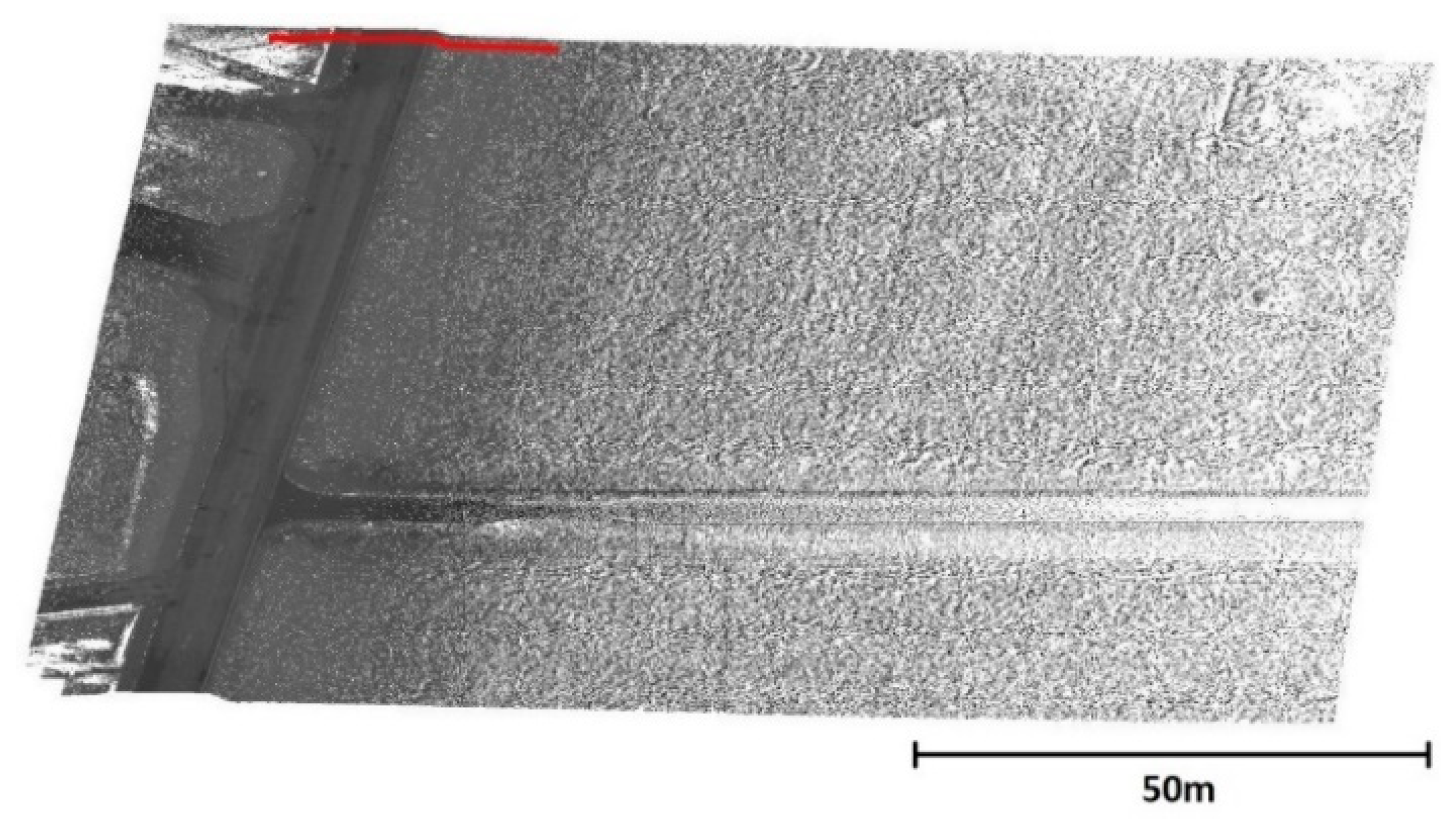
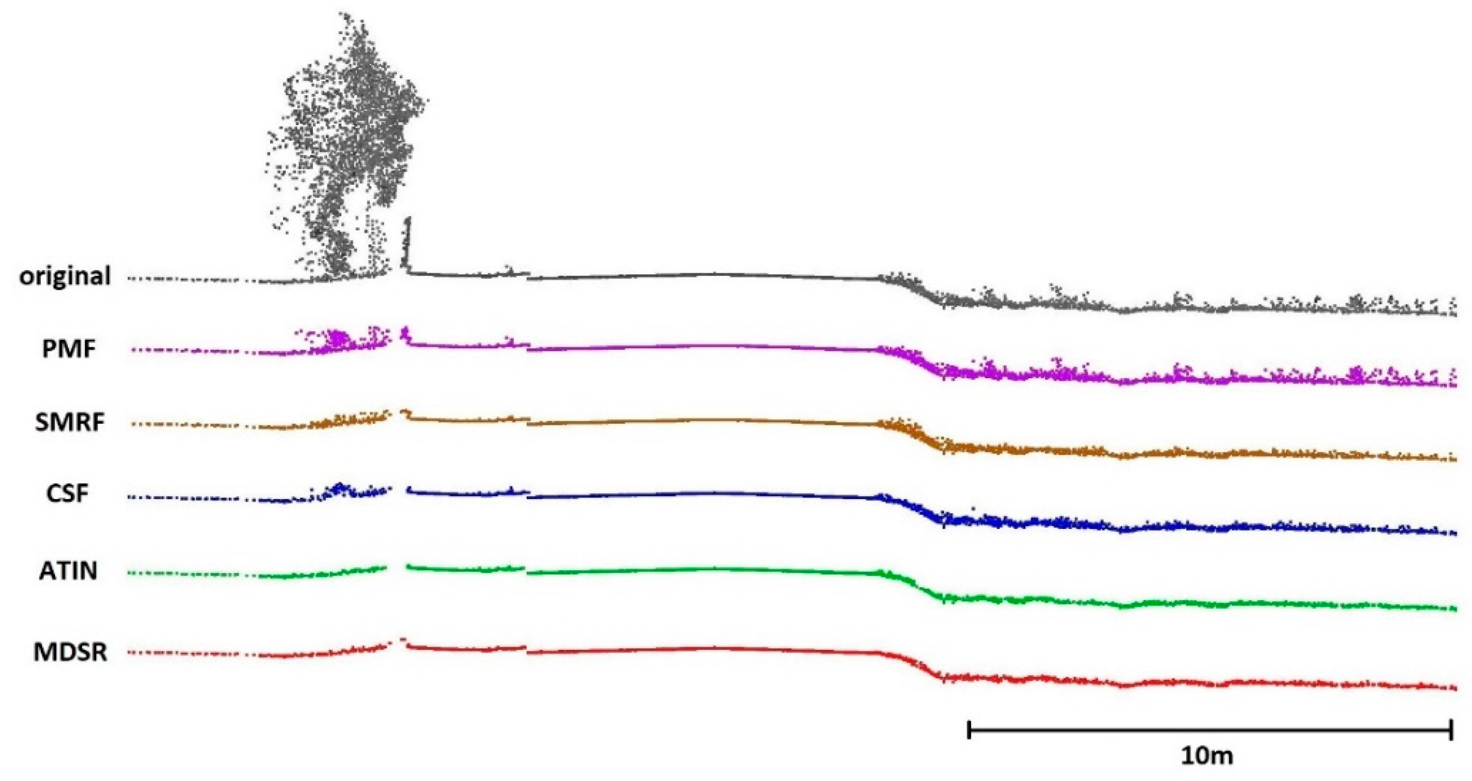
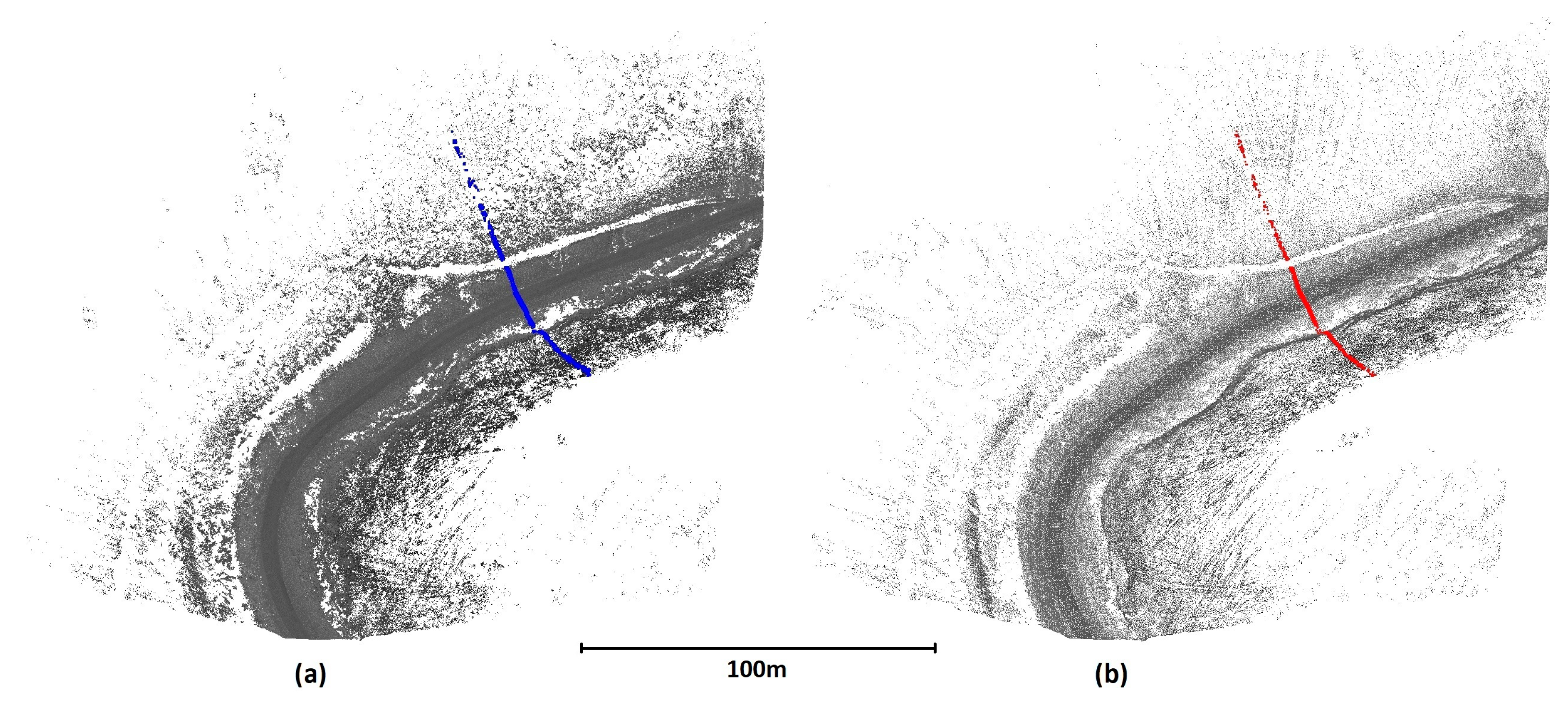
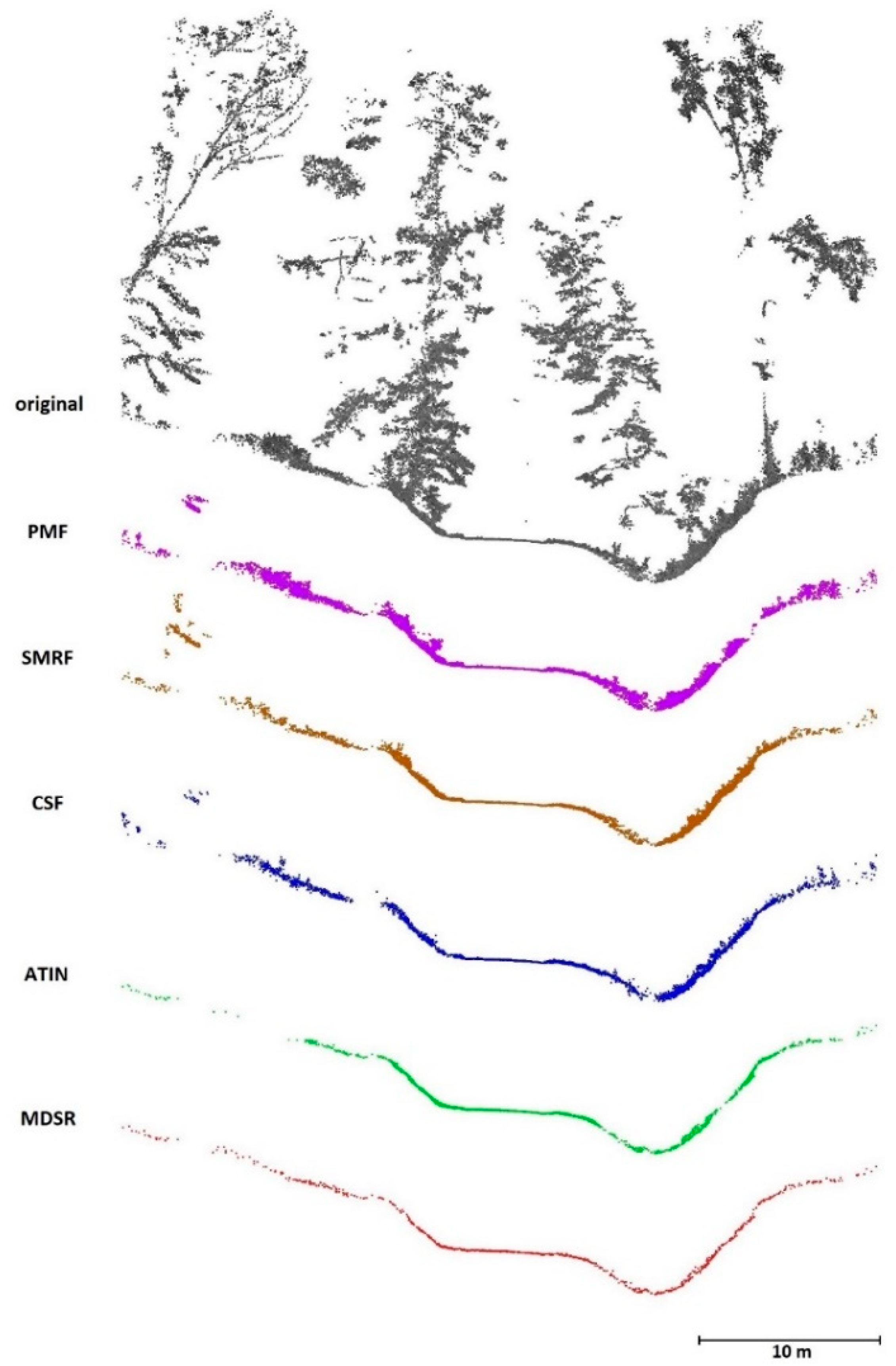
2.6. Visual Evaluation

Visual evaluation of the results of MDSR and those of other filters was performed both on the level of entire surfaces and of profiles from selected potentially problematic areas.

2.7. Evaluation of the Differences from the MDSR-Based Surface

This evaluation was performed as follows: MDSR-filtered data were used for the creation of TIN-approximating ground (MDSR-TIN surface), which was cropped at the edges to remove artifacts described above. The signed distance (+ above and − below) of all points from the original cloud as well as from filtered clouds obtained by other filters was calculated, and root mean square deviations of individual points left below and above the filtering result were calculated.
For the comparison with the original (unfiltered) point cloud, only points below the MDSR-TIN surface are of importance (representing points that were omitted in the detection of the ground), whereas points above the MDSR-TIN surface obviously contain all vegetation.
Subsequently, the results of ground filtering by other filters were evaluated in the same way; in these, however, the RMSD for points above the MDSR-TIN surface was also calculated to evaluate the quality of above-ground point removal. The RMSD was calculated using Equation (1):
RMSD =   d 2 n ,
where d is the distance from the created surface approximation (TIN), and n is the number of points.

3. Results

The above-described filtering techniques were applied on the point clouds; Table 3 shows the number of cloud points before and after filtering using all algorithms.

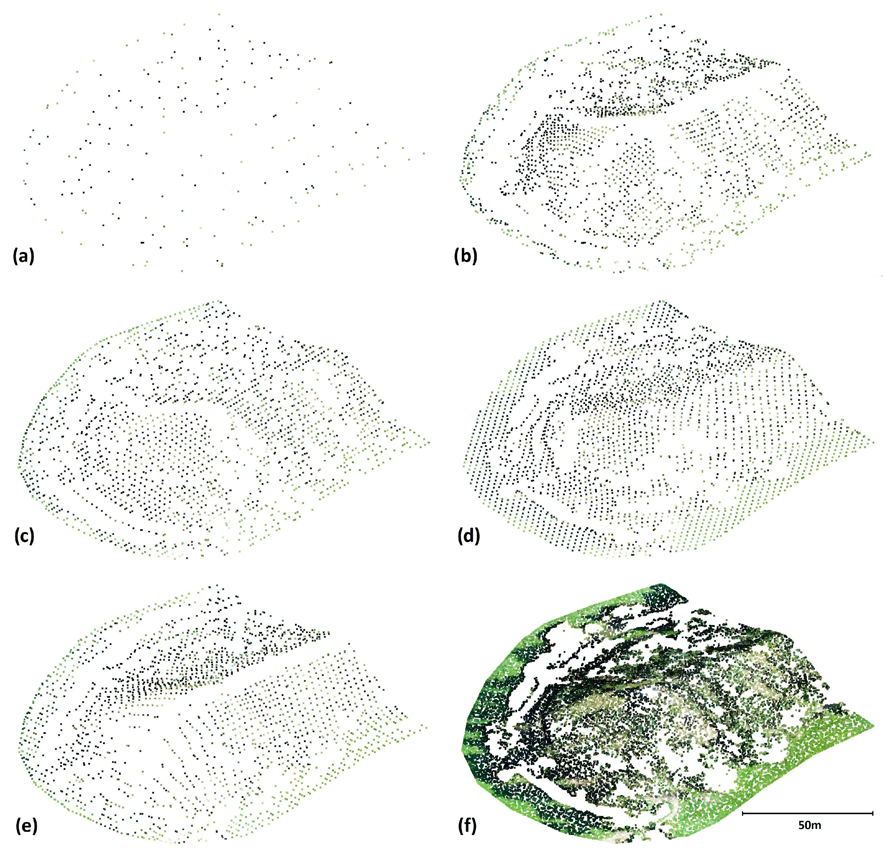
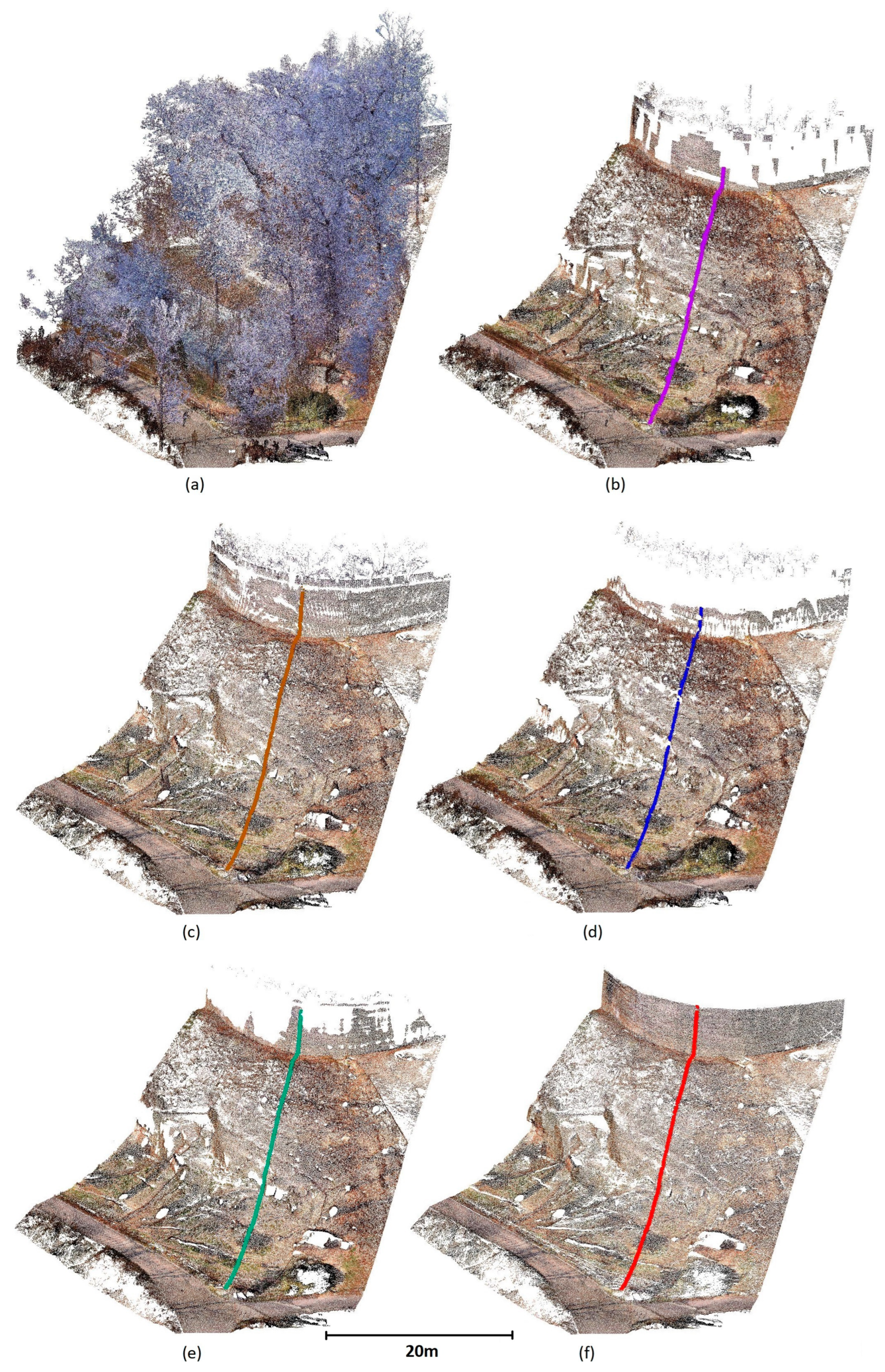
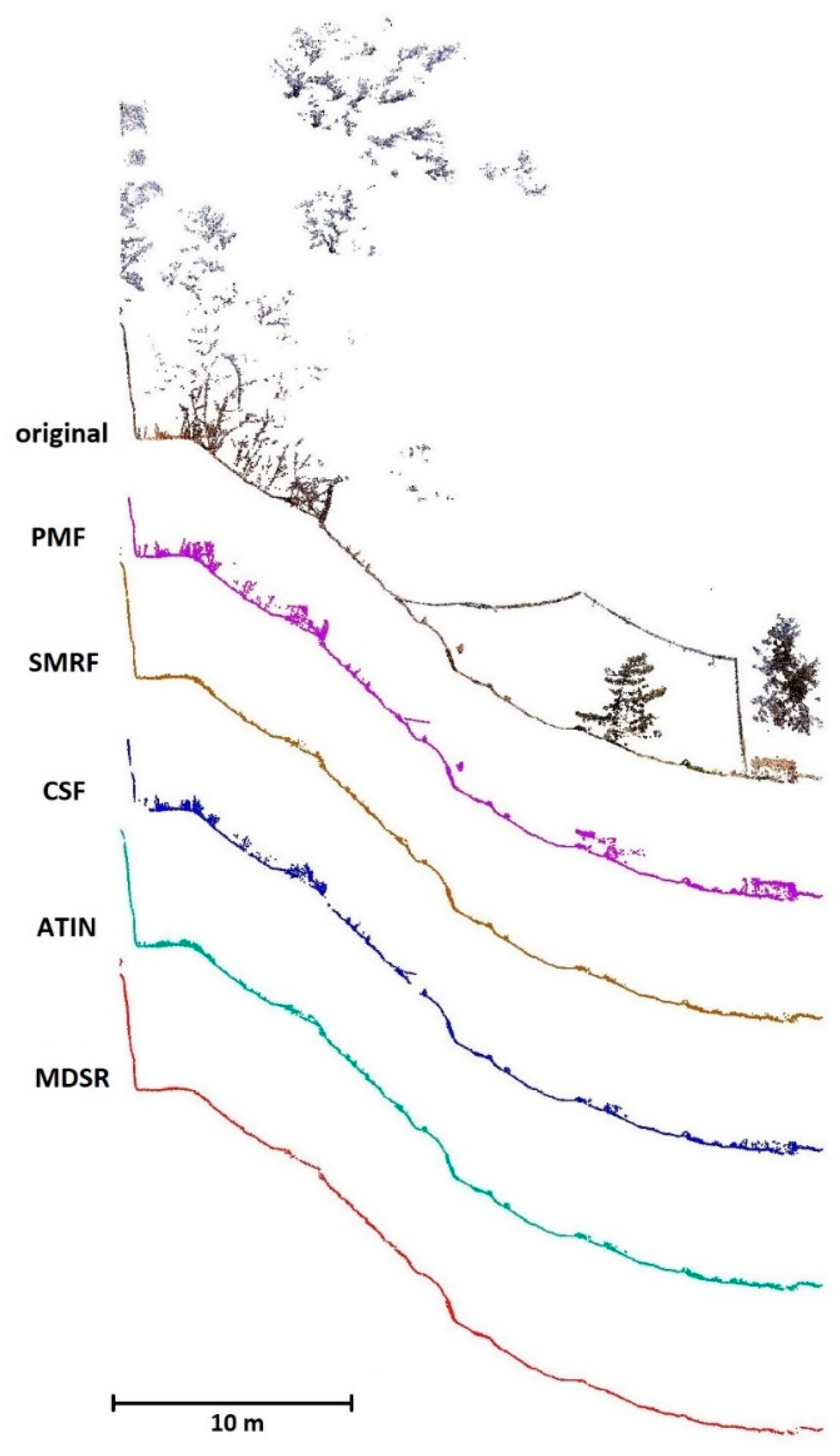
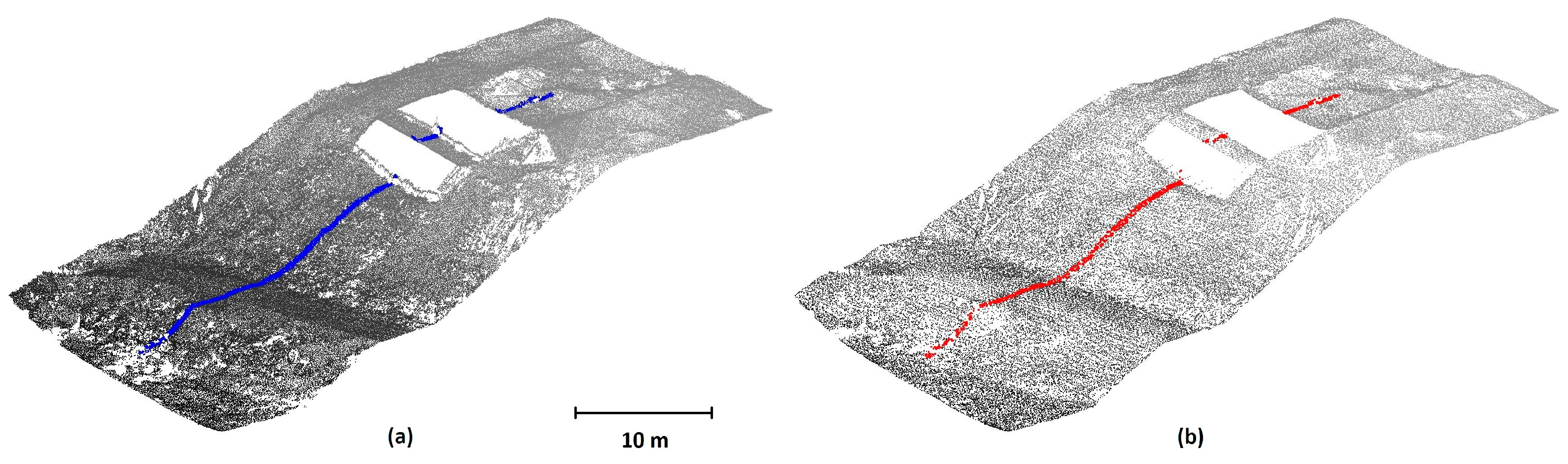
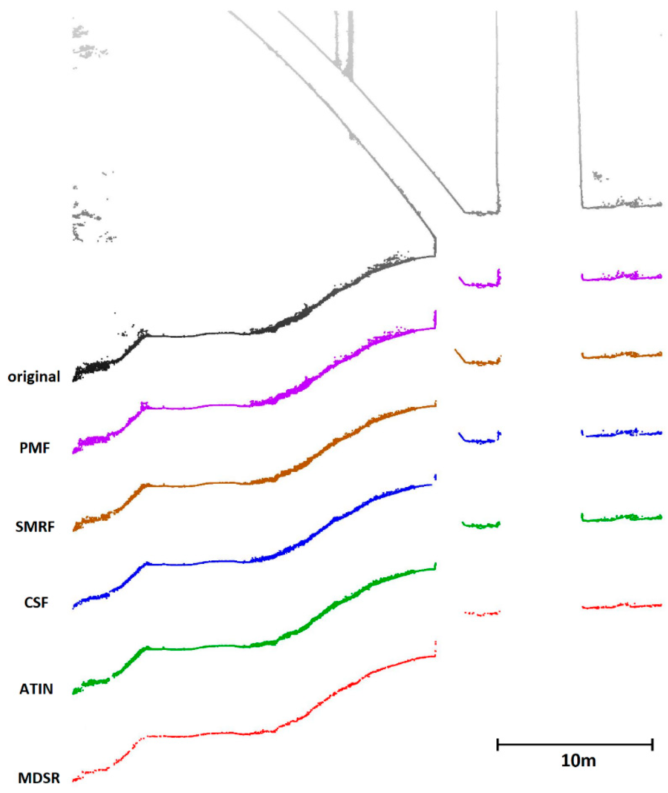
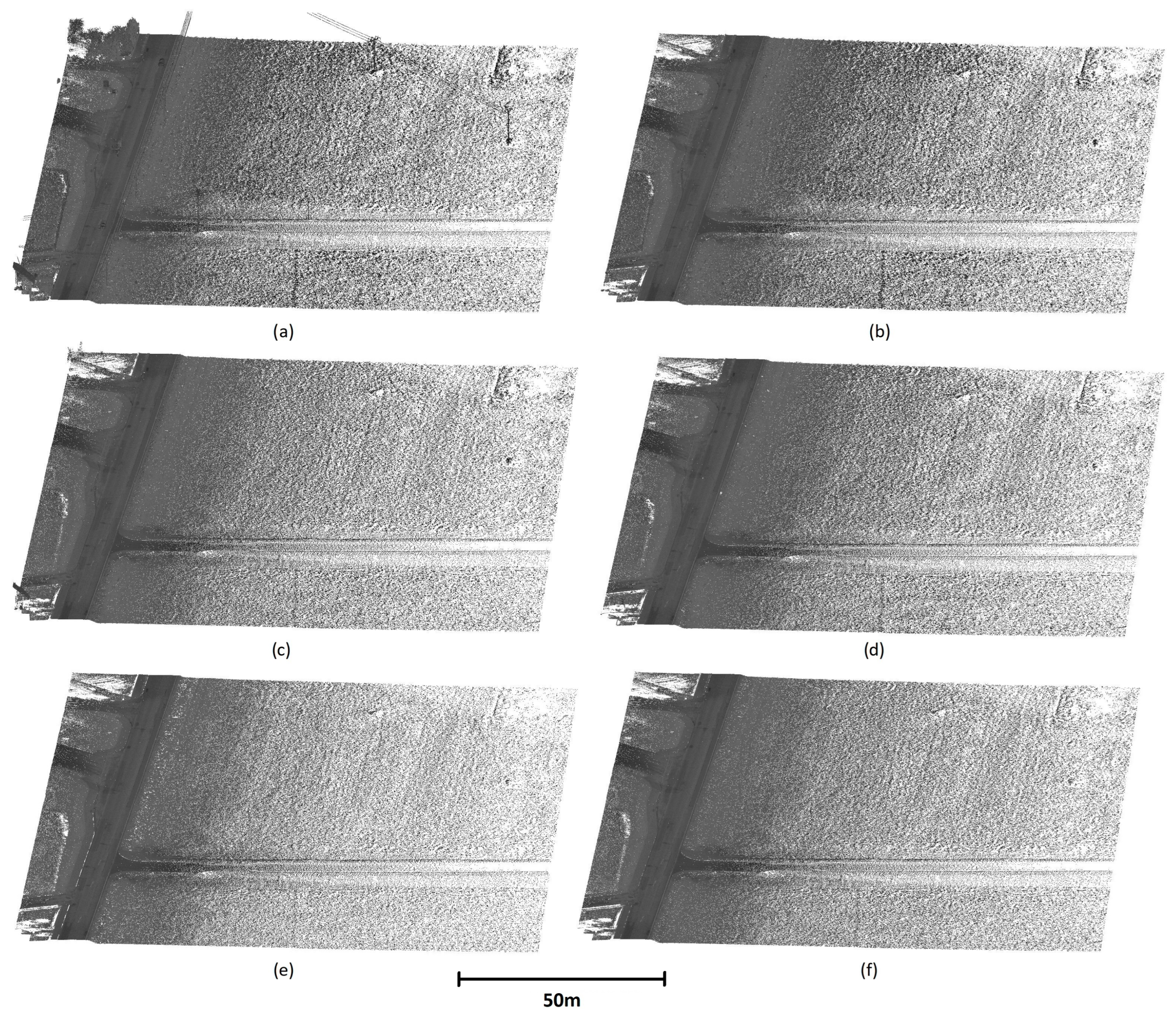
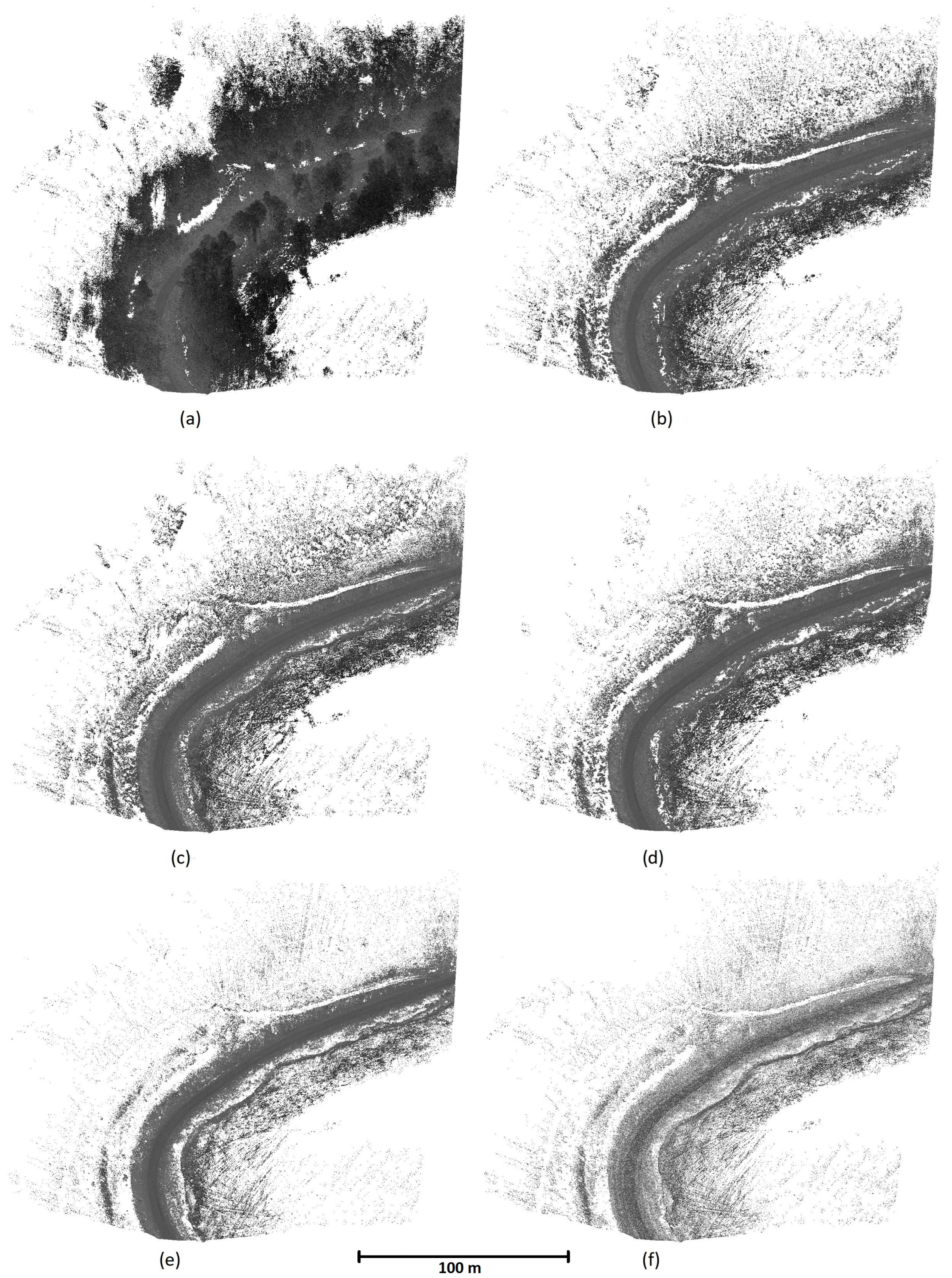
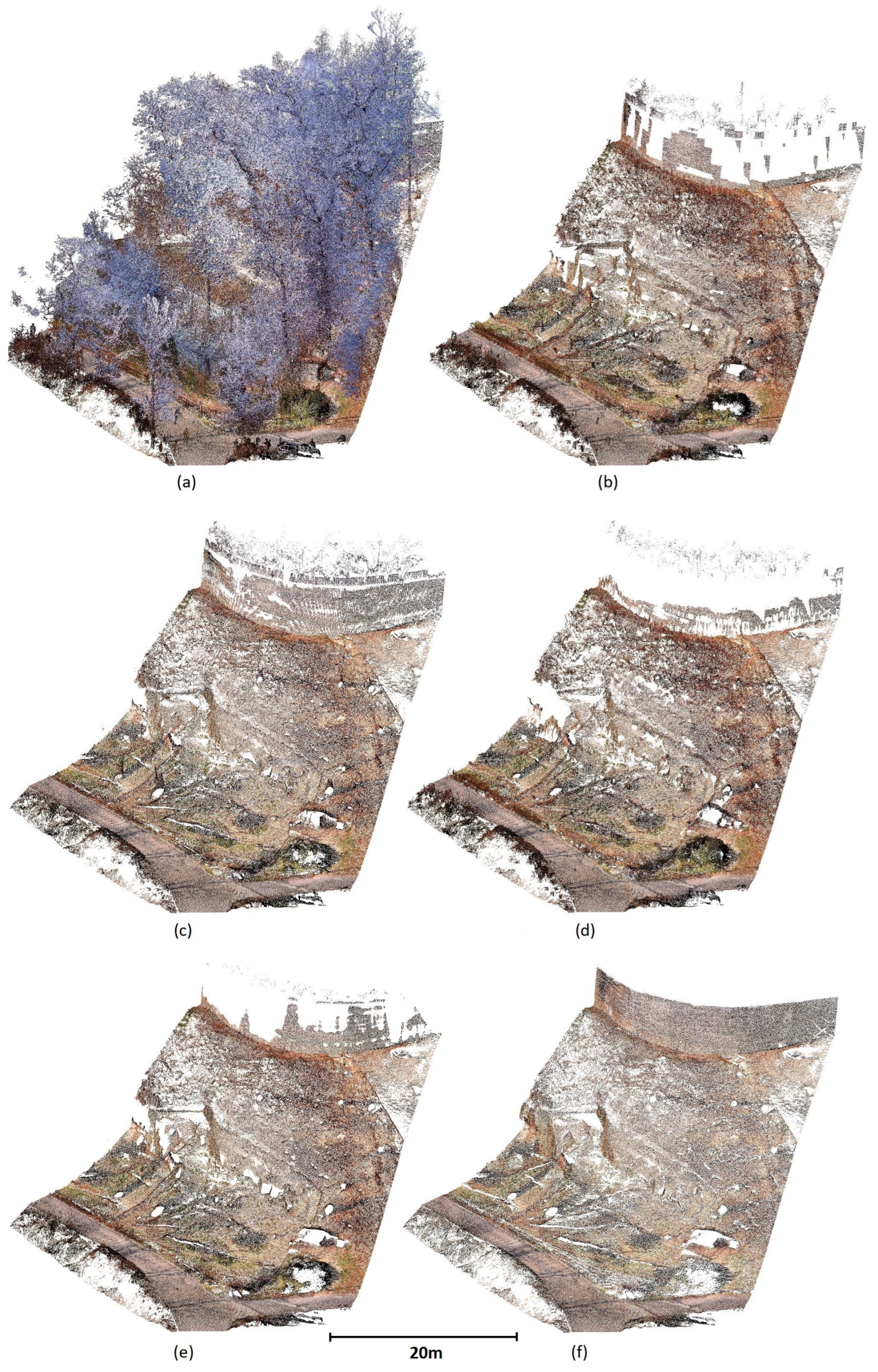
3.1. Visual Evaluation

The first region is practically flat; in principle, any filter should satisfactorily work here. All filters yielded similar results; for this reason, only the result of the MDSR filter is shown (Figure 5).
Since the quality of ground filtering cannot be distinguished when displaying the entire cloud in a single image, it will be presented on selected profiles showing both the original data and data obtained by the filters under comparison (including the MDSR filter). The profile shown in Figure 6 shows the success of both the geometrical filters and MDSR filters in basic filtering. It is worth noting that in parts of the profile with low vegetation (most likely grass), the MDSR profile is significantly smoother (the profile curve aggregates points from a 0.5 m wide strip of the point cloud, and, hence, it cannot be perfectly thin and smooth).
Clearly, the ATIN and MDSR have the best and very similar results, with MDSR results being slightly more complete. Filtering results of all filters are shown in Appendix D.
The second area captured by data 2 is significantly more rugged, covered with dense, both tall and low, vegetation. Ground filtering in this area is no longer a simple matter, the slopes are quite steep, and the point density rapidly decreases with the distance from the vehicle path. The ground surface data are greatly affected by tree cover. An overall view of the CSF and MDSR filtering results is shown in Figure 7. Results of all filters are shown in Appendix D.
After comparing the results, we can conclude practically the same as in the previous case (Figure 8). The MDSR appears to correctly select ground points even in the areas with very sparse data (left and right edges of the image), with the ATIN performing the second best.
The numbers of points of individual filtered point clouds greatly differ (Table 2). While the original cloud consists of 10 mil. points and the CSF a point cloud of 1.25 mil. points, the MDSR identified only 0.28 mil. ground points. However, as can be obviously seen from the figures, even this is sufficient for terrain description. On the road (center), the point density is approximately 45 points/m2; on the adjacent slopes (outside the covered-up areas), there are about 30 points/m2.
It can be, therefore, concluded that the MDSR algorithm in this case successfully filtered the ground and, in addition, suitably and appropriately diluted the point cloud. Such an approximately 1:5 reduction in the number of points in the cloud will bring a significant benefit for the simplification of further processing while not compromising the terrain description (tens of points per square meter are more than sufficient for a high-quality description of the terrain).
The area where data 3 was acquired is a rugged steep cliff, practically vertical in the upper part; it is, therefore, of high complexity and highly problematic for both capture and subsequent evaluation. In such an area, the filtering results differ a lot. For this site, results from all filters are shown, as in this area, the differences in the filtering success are best visible. The data processed by the CSF are visibly full of holes, especially where the terrain slope is higher or under an overhang (center of the left part in the figure).
To capture the ruggedness, shape, and steepness of the area, the grid tilting (explained in Methods) used multiple angles, even as high as 120 deg, which allowed us to capture even the area under the overhang (Figure 9f).
The profiles show similar results as for previous sites, but in this case, the differences are even greater (Figure 10).
In site 4, the surface is somewhat less rugged than in site 3; however, the tall bridge pillars and supports, the contact of which with the terrain is not just perpendicular, represent the dominant filtering problem in this area. The results of CSF and MDSR filtering are shown in Figure 11a,b, respectively. The results of the remaining filters are similar to those of the CSF and are presented in Appendix D (Figure A5).
The profiles in Figure 12 show that even in this anthropomorphic site, the MDSR filter offers the smoothest and thinnest profile of all tested algorithms. Note that in places where the pillars are in contact with the ground, all the filters identify a part of the pillar surfaces as the ground. Again, the MDSR filter performed the best of all used filters (i.e., identifying the smallest area of the pillar surfaces as the ground—only on a single pillar surface).

3.2. Comparison of Point Clouds with an MDSR-Based Surface

The overall RMSDs of points of the original (i.e., unfiltered) point cloud found below the MDSR-generated surface in individual study sites are 0.7 cm, 2.5 cm, 0.6 cm, and 1.7 cm for sites 1, 2, 3, and 4, respectively. This indicates that the MDSR filter indeed selected the lowest points in the cloud. This is comparable with the results of the remaining tested filters, all of which had similar RMSDs of points below the MDSR-generated cloud (Table 4). In other words, all filters were capable of very good detection of the lowest points.
However, when comparing the RMSDs of the filtering results taking into account only the points found above the MDSR-generated surface, the RMSDs of the other filters compared with the MDSR ranged from 4.5 cm to 95 cm, indicating a much higher number of unremoved vegetation points. This can be also seen from the thicker profiles of ground-filtered points yielded by the traditional algorithms compared with the new MDSR filter (Figure 6,Figure 8,Figure 10 and Figure 12). Therefore, of all the five tested filters, the MDSR shows the lowest amount of above-ground points (especially unremoved vegetation) that remained in the clouds after filtering.
On the flat surface (site 1), all filters yielded satisfactory results, whereas at sites 2 and 3, only the ATIN filter performed similarly well as the MDSR filter. In site 4, the situation is different due to the large gaps in ground data caused by the pillars—the bigger pillar is 10 m wide and about 5.5 m long at the point of contact with the ground. To successfully perform, the filters including the MDSR need different settings than in the previous scenarios. This particularly affected the ATIN filter; where the “wilderness” setting that was successfully used in the previous sites (with a default step of 3 m) provided better vegetation filtering but above the gaps, parts of unfiltered pillars (up to the height of 14 m) were filtered as the ground. For this reason, the setting had to be changed to “nature” (default step size of 5 m).
The RMSD above the MDSR surface for the original (unfiltered) point cloud basically shows just the average vegetation height.
The results of the ATIN filter implemented in lasground_new software are the most comparable with those obtained by MDSR filtering; this also corresponds to the profiles shown in the previous chapter.

4. Discussion

Many papers aiming at testing filters and selecting those best suited to the particular purpose have been published. For example, Moudry et al. [42] tested the ground filtering of low-density ALS data capturing a slopy terrain of a spoil heap largely employing the same filters as this paper and comparing the filtering results with control points measured using a total station. Similar to our study, the ATIN also performed very well in their work (root mean square error (RMSE) 0.15 m), followed by the SMRF (0.17 m), PMF (0.18 m), and CSF (0.19 m); nevertheless, the differences between the results of individual filters were relatively small. Štular et al. [49] tested a variety of filters for the determination of the ground from low-density ALS data for archeological purposes. The terrain analyzed in their study was much more rugged with many projections. Again, the ATIN was among the best-performing filters. However, data on the ground filtering of point clouds of a density as high as in our paper capturing rugged areas are practically nonexistent in the literature.
The presented MDSR algorithm works on an entirely different principle compared with not only “classical” geometric filters that create an approximation of the surface using the selected points and then use a threshold to select the terrain points but also other alternative approaches such as that previously presented by our group [45]. Unlike all of these, this algorithm selects the lowest points from the cloud even if only few such points are present, and, as a result of this scarcity of ground points, they fail to form an algorithmically discernible surface necessary for filtering using the above-mentioned approaches.
The main features of our algorithm, therefore, are as follows:
  • No approximations, simplifications, and assumptions of the terrain are made;
  • The filtering step also dilutes the point cloud;
  • Compared with the common geometric filters, this one can be used for much more complex terrains and, therefore, is much more versatile;
  • The computational demands approximately quadratically increase with increasing required detail (due to the number of raster shifts and raster size);
  • Similar to all filtering methods, this one also needs verification by an operator; here, typically, a thin layer of filtering artifacts on the edges of the area needs to be removed either manually or simply by cropping by (typically) several decimeters to a few meters;
  • Where a dense point cloud is needed, the MDSR method could be also used as the first step of an advanced multistep algorithm for the acquisition of the first terrain approximation, after which the remaining points can be identified based on a threshold as in standard filters.
Although this algorithm could work for ALS scanning data, it is primarily designed to work with high-density data of a local character with a high surface density in a complex terrain measured at a short distance (UAV lidar, mobile lidar, terrestrial 3D scanner, SfM method). We should, however, mention a potential pitfall of this algorithm—outliers below the real terrain that the algorithm would detect as terrain points. This is not much of a problem for lidar data used in our paper as during the initial lidar data processing, such outliers are typically removed by the manufacturer-provided software, but this problem might occur when working with SfM data. In such a case, the outliers should be removed by prefiltering using, for example, noise-removal filters.
The algorithm is primarily designed for dense point clouds of nature-close environments (as urban landscapes, typically formed by buildings and planar areas, do not typically need particularly strong vegetation-removal algorithms). However, as illustrated in site 4, which is highly anthropomorphic, the algorithm can work well even in such areas providing that the cell size is set to be larger than the largest gap in the ground points. This, however, has to be compensated by the use of a greater number of stepwise shifts to achieve the terrain model of sufficiently fine detail.
Due to the high computational complexity with a large number of shifts of the base raster, the data can be with advantage gradually reduced. In other words, a smaller window and a smaller number of shifts could be used in the first pass, thus reducing the total number of points (especially above-ground points), and subsequently, a second pass with a larger window and a larger number of shifts could be employed on thus diluted data. Such specific combinations of parameters for stepwise reduction are currently investigated and will be the subject of future papers.

5. Conclusions

The novel MDSR ground-filtering method primarily designed for nature-close areas presented in this paper was proven to be highly effective. Its testing on four point clouds obtained using various methods at sites with varying ruggedness and vegetation cover and comparison of the performance with other widely used filters (ATIN—Lastools; PMF—PDAL; SMRF—PDAL; CSF—CloudCompare) showed it to be superior to those filters (especially in the terrain with the greatest ruggedness and vegetation cover), with the ATIN performing the best of the rest. This was shown both on the visual presentation of the filtered point clouds and by the evaluation of the distance of the MDSR-based surface from the original (unfiltered) point cloud and from the ground data acquired using the other filters.
The selection of the lowest points in various positions and angles leads, besides the identification of the lowest points in the cloud, also to a dilution of the point cloud. Thus, we can assume that the presented filter can be also used in combined approaches with this filter acting as the first step for creating an approximation of the terrain that can be subsequently densified by the standard threshold-based approach employed in other filters. However, it should be noted that as the filter is not designed for urban scenes with large roofs, it is not universally applicable, and for such instances, other filters with a changeable window size, such as the SMRF, might be more suitable.

Author Contributions

Conceptualization, M.Š.; methodology, M.Š.; software, M.Š.; validation, R.U. and L.L.; formal analysis, M.Š. and R.U.; investigation, L.L.; writing—original draft preparation, M.Š.; writing—review and editing, R.U. and L.L.; visualization, M.Š.; funding acquisition, R.U. All authors have read and agreed to the published version of the manuscript.

Funding

This research was funded by the Grant Agency of CTU in Prague—grant number SGS22/046/OHK1/1T/11, “Optimization of acquisition and processing of 3D data for purpose of engineering surveying, geodesy in underground spaces and 3D scanning”, and by the Technology Agency of the Czech Republic—grant number CK03000168, “Intelligent methods of digital data acquisition and analysis for bridge inspections”.

Data Availability Statement

The data presented in this study are available on request from the corresponding author.

Conflicts of Interest

The authors declare no conflict of interest. The funders had no role in the design of the study; in the collection, analyses, or interpretation of data; in the writing of the manuscript; or in the decision to publish the results.

Appendix A. MDSR Algorithm Code

Below, the algorithm pseudocode is shown. The structure of the data is very simple—it is a matrix where details of every point are in a single line, with the first three numbers always representing the point coordinates (X, Y, Z); additional point properties (such as RGB color components, intensity, etc.) are preserved but not used during filtering.
Points =  [ (1) x1 y1 z1 R G B ...
            (2) x2 y2 z2 R G B ...
             .
             .
            (p) xp yp zp R G B ...]
	
First, have a look at the constants and basic functions used in the algorithm:
0. 
Calculation parameters
Raster cell size:
  RasterSize = R
Number of shifts:
  NumberofShifts = N
Shift size
  Shift = R/N
1. 
Reduction of the coordinates of the entire point cloud in a way ensuring that the minimum X, Y, and Z coordinates are equal to zero
function Result = ReduceCoords(Points)
 Xm = min(Points(:,1));
 Ym = min(Points(:,2));
 Zm = min(Points(:,3));
  
  For i = 1:p
    Result(i, :) = Points(i,:) – [Xm Ym Zm]
  end;
End;
  
2. 
Rotation of the entire point cloud by defined angles about individual axes
function Result = RotatePoints(alfa, beta, gama, Points)
 RotX = [1      0         0;
        0  cos(alfa)  sin(alfa);
        0 -sin(alfa)  cos(alfa)]
 RotY = [cos(beta)  0   -sin(beta);
            0      1       0;
        sin(beta)  0    cos(beta)]
 RotZ = [cos(gama)  sin(gama)   0;
        -sin(gama) cos(gama)   0;
           0          0        1]
 Rot = RotZ*RotX*RotY;
  
 For i = 1:p
    Result(i, :) = (Rot*Points(i,:)’)’
 end;
End;
3. 
Shift of the X and Y coordinates by a predefined value
function Result = ShiftPoints(Sx, Sy, Points)
  For i = 1:p
    Result(i,:) = Points(i,:) + [Sx Sy 0]
  end;
End;
			  
4. 
Search for the point with the lowest elevation in each raster cell
function rastr = Rasterize(RasterSize, Points)
 max_x = max(Points(:,1));
 max_y = max(Points(:,2));
  
 limit_x = ceil(max_x/ RasterSize);
 limit_y = ceil(max_y/ RasterSize);
 rastr = zeros((limit_x, limit_y);
   
 for i = 1:p do
    x = floor(Points(i,1)/RasterSize)+1;
    y = floor(Points(i,2)/RasterSize)+1;
    if rastr(x,y) == 0 then
        rastr(x,y) = i
       else
           if Points(i,3) < Points(rastr(x,y),3) then
               rastr(x,y) = i;
           end;
       end;
 end;
End;
			  
5. 
Saving the identified data—this is solely a routine programming issue of data management
function result = SaveLowestPoints(LPointsID, Points)
//here, the storage pathways and form are to be programmed.
End;
			   
6. 
The program itself
PointsC = ReduceCoords(Points)
For alfa = [alfa1, alfa2, …, alfam]
 For beta = [beta1, beta2, …, betan]
  For gama = [gama1, gama2, …, gamao]
     PointsR = RotatePoints(alfa, beta, gama, PointsC)
     PointsR = ReduceCoords(PointsR)
     For SX = 0:N
        For SY = 0:N
           PointsS = ShiftPoints(SX*Shift, SY*Shift)
	           LowestPointsID = Rasterize(RasterSize, PointsS)
	           SaveLowestPoints(LowestPointsID, Points)
        end;
     end;
  end;
 end;
end;
			 
PointsC = ReduceCoords(Points)
For alfa = [alfa1, alfa2, …, alfam]
 For beta = [beta1, beta2, …, betan]
 For gama = [gama1, gama2, …, gamao]
  PointsR = RotatePoints(alfa, beta, gama, PointsC)
  PointsR = ReduceCoords(PointsR)
  For SX = 0:N
   For SY = 0:N
   PointsS = ShiftPoints(SX*Shift, SY*Shift)
   LowestPointsID = Rasterize(RasterSize, PointsS)
   SaveLowestPoints(LowestPointsID, Points)
   end;
  end;
 end;
 end;
end;

Appendix B. MDSR Algorithm Flowchart

Figure A1. MDSR Algorithm flowchart.
Remotesensing 14 04916 g0a1

Appendix C. Scanning Systems Used for Data Acquisition

  • DJI Zenmuse L1 UAV Scanner
For the acquisition of the illustration dataset, the UAV scanner DJI Zenmuse L1 was used. It was mounted on a DJI Matrice 300 quadrocopter, and the basic characteristics of both devices are given below in Table A1 and Table A2. Further information can be found on the manufacturer’s website (https://www.dji.com, accessed on 6 May 2022).
Table A1. Basic characteristics of DJI Zenmuse L1 laser scanner.
Dimensions152 × 110 × 169 mm
Weight930 ± 10 g
Maximum measurement distance450 m at 80% reflectivity
Recording speed190 m at 10% reflectivity
System accuracy (1σ)Single return: max. 240,000 points/s
Distance measurement accuracy (1σ)Multiple return: max. 480,000 points/s
Beam divergenceHorizontal: 10 cm per 50 m
Maximum registered reflectionsVertical: 5 cm per 50 m
RGB camera sensor size3 cm per 100 m
RGB camera effective pixels0.28° (vertical) × 0.03° (horizontal)
Table A2. Basic characteristics of UAV DJI Matrice 300.
WeightApprox. 6.3 kg (with one gimbal)
Max. transmitting distance (Europe)8 km
Max. flight time55 min
Dimensions810 × 670 × 430 mm
Max. payload2.7 kg
Max. speed82 km/h
  • Leica Pegasus Mobile Scanner
For the acquisition of the point cloud on sites 1 and 2, the mobile system Leica Pegasus Two was used; the basic characteristics of the device are given below in Table A3. Further information can be found on the manufacturer’s website (https://leica-geosystems.com/, accessed on 6 May 2022).
Table A3. Basic characteristics of Leica Pegasus Two scanner.
Weight51 kg
Dimensions60 × 76 × 68 cm
Typical horizontal accuracy (RMS)0.020 m
Typical horizontal accuracy (RMS)0.015 m
Laser scannerZF 9012
Scanner frequency1 mil points per second
Other accessories and featuresCameras
IMU
Wheel sensor
GNSS—GPS and GLONASS
  • Trimble X7 Terrestrial Scanner
For the acquisition of the point cloud on site 3, the 3D terrestrial scanner Trimble X7 was used; the basic characteristics of the device are given below in Table A4. Further information can be found on the manufacturer’s website (https://geospatial.trimble.com, accessed on 6 May 2022).
Table A4. Basic characteristics of Trimble X7 3D scanner.
Weight5.8 kg
Dimensions178 mm × 353 mm × 170 mm
Laser wavelength1550 nm
Field of view360° × 282°
Scan speedUp to 500 kHz
Range measurement principleTime-of-flight
Range noise<2.5 mm/30 m
Range accuracy (1 sigma)2 mm
Angular accuracy (1 sigma)21″
Other important featuresSensors’ autocalibration
3 coaxial calibrated 10 MPix cameras
Automatic level compensation
(in range ±10°)
Inertial navigation system for autoregistration
  • Leica P40 Terrestrial Scanner
For the acquisition of the point cloud on site 4, the 3D terrestrial scanner Leica P40 was used; the basic characteristics of the device are given below in Table A5. Further information can be found on the manufacturer’s website (https://leica-geosystems.com, accessed on 6 May 2022).
Table A5. Basic characteristics of Leica P40 scanner.
Weight12.25 kg
Dimensions238 mm × 358 mm × 395 mm
Laser wavelength1550 nm/658 nm
Field of view360° × 290°
Scan speedUp to 1 mil point/s
Range measurement principleTime-of-flight
Range accuracy (1 sigma)1.2 mm + 10 ppm
Angular accuracy (1 sigma)8″
Other important featuresDual-axis compensator (accuracy 1.5″)
Internal camera 4 MP per each 17° × 17°, color image; 700 MP for panoramic image
  • DJI Phantom 4 RTK
For the acquisition of the point cloud on site 4 also, the DJI Phantom 4 RTK UAV was used; the basic characteristics of the device are given below in Table A6. Further information can be found on the manufacturer’s website (https://dji.com, accessed on 6 May 2022).
Table A6. Basic characteristics of DJI Phantom 4 RTK UAV.
Weight1.391 g
Max. transmitting distance (Europe)5 km
Max. flight time30 min
Dimensions250 × 250 × 200 mm (approx.)
Max. speed58 km/h
Camera resolution4864 × 3648

Appendix D. Filtering Results for All Sites and Filters

Figure A2. Results of filtering of site 1: (a) original data, (b) after PMF filtering, (c) after SMRF filtering, (d) after CSF filtering, (e) after ATIN filtering, and (f) after MDSR filtering.
Remotesensing 14 04916 g0a2
Figure A3. Results of filtering of site 2: (a) original data, (b) after PMF filtering, (c) after SMRF filtering, (d) after CSF filtering, (e) after ATIN filtering, and (f) after MDSR filtering.
Remotesensing 14 04916 g0a3
Figure A4. Results of filtering of site 1: (a) original data, (b) after PMF filtering, (c) after SMRF filtering, (d) after CSF filtering, (e) after ATIN filtering, and (f) after MDSR filtering.
Remotesensing 14 04916 g0a4
Figure A5. Results of filtering of site 4: (a) original data, (b) after PMF filtering, (c) after SMRF filtering, (d) after CSF filtering, (e) after ATIN filtering, and (f) after MDSR filtering.
Remotesensing 14 04916 g0a5

References

  1. Pukanska, K.; Bartos, K.; Hideghety, A.; Kupcikova, K.; Ksenak, L.; Janocko, J.; Gil, M.; Frackiewicz, P.; Prekopová, M.; Ďuriska, I.; et al. Hardly Accessible Morphological Structures—Geological Mapping and Accuracy Analysis of SfM and TLS Surveying Technologies. Acta Montan. Slovaca 2020, 25, 479–493, ISSN 1335-1788. [Google Scholar] [CrossRef]
  2. Kalvoda, P.; Nosek, J.; Kuruc, M.; Volařík, T.; Kalvodova, P. Accuracy Evaluation and Comparison of Mobile Laser Scanning and Mobile Photogrammetry Data; IOP Conference Series: Earth and Environmental Science; IOP Publishing Ltd.: Bristol, UK, 2020; pp. 1–10. ISSN 1755-1307. [Google Scholar] [CrossRef]
  3. Štroner, M.; Urban, R.; Línková, L. A New Method for UAV Lidar Precision Testing Used for the Evaluation of an Affordable DJI ZENMUSE L1 Scanner. Remote Sens. 2021, 13, 4811. [Google Scholar] [CrossRef]
  4. Guillaume, A.S.; Leempoel, K.; Rochat, E.; Rogivue, A.; Kasser, M.; Gugerli, F.; Parisod, C.; Joost, S. Multiscale Very High Resolution Topographic Models in Alpine Ecology: Pros and Cons of Airborne LiDAR and Drone-Based Stereo-Photogrammetry Technologies. Remote Sens. 2021, 13, 1588. [Google Scholar] [CrossRef]
  5. Jon, J.; Koska, B.; Pospíšil, J. Autonomous Airship Equipped with Multi-Sensor Mapping Platform. ISPRS Int. Arch. Photogramm. Remote Sens. Spat. Inf. Sci. 2013, 40, 119–124, ISSN 2194-9034. [Google Scholar] [CrossRef] [Green Version]
  6. Berrett, B.E.; Vernon, C.A.; Beckstrand, H.; Pollei, M.; Markert, K.; Franke, K.W.; Hedengren, J.D. Large-Scale Reality Modeling of a University Campus Using Combined UAV and Terrestrial Photogrammetry for Historical Preservation and Practical Use. Drones 2021, 5, 136. [Google Scholar] [CrossRef]
  7. McMahon, C.; Mora, O.E.; Starek, M.J. Evaluating the Performance of sUAS Photogrammetry with PPK Positioning for Infrastructure Mapping. Drones 2021, 5, 50. [Google Scholar] [CrossRef]
  8. Le Van Canh, X.; Cao Xuan Cuong, X.; Nguyen Quoc Long, X.; Le Thi Thu Ha, X.; Tran Trung Anh, X.; Xuan-Nam Bui, X. Experimental Investigation on the Performance of DJI Phantom 4 RTK in the PPK Mode for 3D Mapping Open-Pit Mines. Inz. Miner.-J. Pol. Miner. Eng. Soc. 2020, 1, 65–74, ISSN 1640-4920. [Google Scholar] [CrossRef]
  9. Fagiewicz, K.; Lowicki, D. The Dynamics of Landscape Pattern Changes in Mining Areas: The Case Study of The Adamow-Kozmin Lignite Basin. Quaest. Geogr. 2019, 38, 151–162, ISSN 0137-477X. [Google Scholar] [CrossRef] [Green Version]
  10. Zimmerman, T.; Jansen, K.; Miller, J. Analysis of UAS Flight Altitude and Ground Control Point Parameters on DEM Accuracy along a Complex, Developed Coastline. Remote Sens. 2020, 12, 2305. [Google Scholar] [CrossRef]
  11. Brunier, G.; Oiry, S.; Gruet, Y.; Dubois, S.F.; Barillé, L. Topographic Analysis of Intertidal Polychaete Reefs (Sabellaria alveolata) at a Very High Spatial Resolution. Remote Sens. 2022, 14, 307. [Google Scholar] [CrossRef]
  12. Taddia, Y.; González-García, L.; Zambello, E.; Pellegrinelli, A. Quality Assessment of Photogrammetric Models for Façade and Building Reconstruction Using DJI Phantom 4 RTK. Remote Sens. 2020, 12, 3144. [Google Scholar] [CrossRef]
  13. Kavaliauskas, P.; Židanavičius, D.; Jurelionis, A. Geometric Accuracy of 3D Reality Mesh Utilization for BIM-Based Earthwork Quantity Estimation Workflows. ISPRS Int. J. Geo-Inf. 2021, 10, 399. [Google Scholar] [CrossRef]
  14. Schroder, W.; Murtha, T.; Golden, C.; Scherer, A.K.; Broadbent, E.N.; Almeyda Zambrano, A.M.; Herndon, K.; Griffin, R. UAV LiDAR Survey for Archaeological Documentation in Chiapas, Mexico. Remote Sens. 2021, 13, 4731. [Google Scholar] [CrossRef]
  15. Blistan, P.; Kovanic, L.; Patera, M.; Hurcik, T. Evaluation quality parameters of DEM generated with low-cost UAV photogrammetry and Structure-from-Motion (SfM) approach for topographic surveying of small areas. Acta Montan. Slovaca 2019, 24, 198–212, ISSN 1335-1788. [Google Scholar]
  16. Nesbit, P.R.; Hubbard, S.M.; Hugenholtz, C.H. Direct Georeferencing UAV-SfM in High-Relief Topography: Accuracy Assessment and Alternative Ground Control Strategies Along Steep Inaccessible Rock Slopes. Remote Sens. 2022, 14, 490. [Google Scholar] [CrossRef]
  17. Vosselman, G. Slope based filtering of laser altimetry data. Int. Arch. Photogramm. Remote Sens. 2000, 33, 935–942. [Google Scholar]
  18. Sithole, G. Filtering of laser altimetry data using a slope adaptive filter. Int. Arch. Photogramm. Remote Sens. 2001, 34, 203–210. [Google Scholar]
  19. Susaki, J. Adaptive Slope Filtering of Airborne LiDAR Data in Urban Areas for Digital Terrain Model (DTM) Generation. Remote Sens. 2012, 4, 1804–1819. [Google Scholar] [CrossRef] [Green Version]
  20. Kraus, K.; Pfeifer, N. Determination of terrain models in wooded areas with airborne laser scanner data. ISPRS J. Photogramm. Remote Sens. 1998, 53, 193–203. [Google Scholar] [CrossRef]
  21. Axelsson, P. DEM generation from laser scanner data using adaptive TIN models. Int. Arch. Photogramm. Remote Sens. 2000, 33, 111–118. [Google Scholar]
  22. Kobler, A.; Pfeifer, N.; Ogrinc, P.; Todorovski, L.; Ostir, K.; Dzeroski, S. Repetitive interpolation: A robust algorithm for DTM generation from Aerial Laser Scanner Data in forested terrain. Remote Sens. Environ. 2007, 108, 9–23. [Google Scholar] [CrossRef]
  23. Zhang, K.; Chen, S.C.; Whitman, D.; Shyu, M.L.; Yan, J.; Zhang, C. A progressive morphological filter for removing nonground measurements from airborne LIDAR data. IEEE Trans. Geosci. Remote Sens. 2003, 41, 872–882. [Google Scholar] [CrossRef] [Green Version]
  24. Pingel, T.J.; Clarke, K.C.; McBride, W.A. An improved simple morphological filter for the terrain classification of airborne LIDAR data. ISPRS J. Photogramm. Remote Sens 2013, 77, 21–30. [Google Scholar] [CrossRef]
  25. Li, Y. Filtering Airborne LIDAR Data by AN Improved Morphological Method Based on Multi-Gradient Analysis. ISPRS Int. Arch. Photogramm. Remote Sens. Spat. Inf. Sci. 2013, 40, 191–194. [Google Scholar] [CrossRef] [Green Version]
  26. Im, J.; Jensen, J.R.; Hodgson, M.E. Object-based land cover classification using high-posting-density LiDAR data. GIScience Remote Sens. 2008, 45, 209–228. [Google Scholar] [CrossRef] [Green Version]
  27. Zhang, J.; Lin, X.; Ning, X. SVM-Based Classification of Segmented Airborne LiDAR Point Clouds in Urban Areas. Remote Sens. 2013, 5, 3749–3775. [Google Scholar] [CrossRef] [Green Version]
  28. Tovari, D.; Pfeifer, N. Segmentation based robust interpolation—A new approach to laser data filtering. Int. Arch. Photogramm. Remote Sens. Spat. Inf. Sci. 2005, 36, 79–84. [Google Scholar]
  29. Vosselman, G.; Coenen, M.; Rottensteiner, F. Contextual segment-based classification of airborne laser scanner data. ISPRS J. Photogramm. Remote Sens. 2017, 128, 354–371. [Google Scholar] [CrossRef]
  30. Bartels, M.; Wei, H. Segmentation of LiDAR data using measures of distribution. Int. Arch. Photogramm. Remote Sens. Spat. Inf. Sci. 2006, 36, 426–431. [Google Scholar]
  31. Crosilla, F.; Macorig, D.; Scaioni, M.; Sebastianutti, I.; Visintini, D. LiDAR data filtering and classification by skewness and kurtosis iterative analysis of multiple point cloud data categories. Appl. Geomat. 2013, 5, 225–240. [Google Scholar] [CrossRef] [Green Version]
  32. Buján, S.; Cordero, M.; Miranda, D. Hybrid Overlap Filter for LiDAR Point Clouds Using Free Software. Remote Sens. 2020, 12, 1051. [Google Scholar] [CrossRef] [Green Version]
  33. Zhang, W.; Qi, J.; Wan, P.; Wang, H.; Xie, D.; Wang, X.; Yan, G. An easy-to-use airborne LiDAR data filtering method based on cloth simulation. Remote Sens. 2016, 8, 501. [Google Scholar] [CrossRef]
  34. Rizaldy, A.; Persello, C.; Gevaert, C.; Oude Elberink, S.; Vosselman, G. Ground and Multi-Class Classification of Airborne Laser Scanner Point Clouds Using Fully Convolutional Networks. Remote Sens. 2018, 10, 1723. [Google Scholar] [CrossRef] [Green Version]
  35. Zhang, J.; Hu, X.; Dai, H.; Qu, S. DEM Extraction from ALS Point Clouds in Forest Areas via Graph Convolution Network. Remote Sens. 2020, 12, 178. [Google Scholar] [CrossRef] [Green Version]
  36. Cai, S.; Zhang, W.; Liang, X.; Wan, P.; Qi, J.; Yu, S.; Yan, G.; Shao, J. Filtering Airborne LiDAR Data Through Complementary Cloth Simulation and Progressive TIN Densification Filters. Remote Sens. 2019, 11, 1037. [Google Scholar] [CrossRef] [Green Version]
  37. Hu, X.; Yuan, Y. Deep-Learning-Based Classification for DTM Extraction from ALS Point Cloud. Remote Sens. 2016, 8, 730. [Google Scholar] [CrossRef] [Green Version]
  38. Jakovljevic, G.; Govedarica, M.; Alvarez-Taboada, F.; Pajic, V. Accuracy Assessment of Deep Learning Based Classification of LiDAR and UAV Points Clouds for DTM Creation and Flood Risk Mapping. Geosciences 2019, 9, 323. [Google Scholar] [CrossRef] [Green Version]
  39. Yang, Z.; Jiang, W.; Lin, Y.; Elberink, S.O. Using Training Samples Retrieved from a Topographic Map and Unsupervised Segmentation for the Classification of Airborne Laser Scanning Data. Remote Sens. 2020, 12, 877. [Google Scholar] [CrossRef] [Green Version]
  40. Li, H.; Ye, W.; Liu, J.; Tan, W.; Pirasteh, S.; Fatholahi, S.N.; Li, J. High-Resolution Terrain Modeling Using Airborne LiDAR Data with Transfer Learning. Remote Sens. 2021, 13, 3448. [Google Scholar] [CrossRef]
  41. Na, J.; Xue, K.; Xiong, L.; Tang, G.; Ding, H.; Strobl, J.; Pfeifer, N. UAV-Based Terrain Modeling under Vegetation in the Chinese Loess Plateau: A Deep Learning and Terrain Correction Ensemble Framework. Remote Sens. 2020, 12, 3318. [Google Scholar] [CrossRef]
  42. Moudrý, V.; Klápště, P.; Fogl, M.; Gdulová, K.; Barták, V.; Urban, R. Assessment of LiDAR ground filtering algorithms for determining ground surface of non-natural terrain overgrown with forest and steppe vegetation. Measurement 2020, 150, 107047. [Google Scholar] [CrossRef]
  43. Chen, C.; Guo, J.; Wu, H.; Li, Y.; Shi, B. Performance Comparison of Filtering Algorithms for High-Density Airborne LiDAR Point Clouds over Complex LandScapes. Remote Sens. 2021, 13, 2663. [Google Scholar] [CrossRef]
  44. Klápště, P.; Fogl, M.; Barták, V.; Gdulová, K.; Urban, R.; Moudrý, V. Sensitivity analysis of parameters and contrasting performance of ground filtering algorithms with UAV photogrammetry-based and LiDAR point clouds. Int. J. Digit. Earth 2020, 13, 1672–1694. [Google Scholar] [CrossRef]
  45. Štroner, M.; Urban, R.; Lidmila, M.; Kolář, V.; Křemen, T. Vegetation Filtering of a Steep Rugged Terrain: The Performance of Standard Algorithms and a Newly Proposed Workflow on an Example of a Railway Ledge. Remote Sens. 2021, 13, 3050. [Google Scholar] [CrossRef]
  46. Wang, Y.; Koo, K. Vegetation Removal on 3D Point Cloud Reconstruction of Cut-Slopes Using U-Net. Appl. Sci. 2022, 12, 395. [Google Scholar] [CrossRef]
  47. Mohamad, N.; Ahmad, A.; Khanan, M.; Din, A. Surface Elevation Changes Estimation Underneath Mangrove Canopy Using SNERL Filtering Algorithm and DoD Technique on UAV-Derived DSM Data. ISPRS Int. J. Geo-Inf. 2022, 11, 32. [Google Scholar] [CrossRef]
  48. Hui, Z.; Jin, S.; Xia, Y.; Nie, Y.; Xie, X.; Li, N. A mean shift segmentation morphological filter for airborne LiDAR DTM extraction under forest canopy. Opt. Laser Technol. 2021, 136, 106728. [Google Scholar] [CrossRef]
  49. Štular, B.; Lozić, E. Comparison of Filters for Archaeology-Specific Ground Extraction from Airborne LiDAR Point Clouds. Remote Sens. 2020, 12, 3025. [Google Scholar] [CrossRef]
Figure 1. Principle of the method: (ac) vertical raster in 3 steps (i.e., shifted 3 times)—red points; (df) rotated raster in 3 steps (i.e., one rotation shifted 3 times)—blue points; (g) resulting terrain points identified in the respective color.
Remotesensing 14 04916 g001
Figure 2. Illustration dataset: (a) true colors and (b) elevation-coded data.
Remotesensing 14 04916 g002
Figure 3. Illustration data—gradual processing: (a) vertical grid—only the first step; (b) vertical grid—5 × 5 steps; (ce) after one selected rotation—5 × 5 steps; and (f) resulting ground point cloud constructed from all positional shifts and rotations.
Remotesensing 14 04916 g003
Figure 4. Testing point clouds colored by relative height: (a) site 1, (b) site 2, (c) site 3, and (d) site 4.
Remotesensing 14 04916 g004
Figure 5. Site 1: data after MDSR filtering; red line indicates locations of profiles presented in Figure 6.
Remotesensing 14 04916 g005
Figure 6. Site 1—profile; gray—original cloud; purple—PMF; brown—SMRF; blue—CSF; green—ATIN; red—MDSR.
Remotesensing 14 04916 g006
Figure 7. Site 2 after (a) CSF and (b) MDSR filtering; the profiles detailed in Figure 8 are indicated by blue (CSF) and red (MDSR) lines.
Remotesensing 14 04916 g007
Figure 8. Profiles from site 2 filtering: gray—original cloud; purple—PMF; brown—SMRF; blue—CSF; green—ATIN; red—MDSR.
Remotesensing 14 04916 g008
Figure 9. Site 3: (a) original, (b) after PMF filtering, (c) after SMRF filtering, (d) after CSF filtering, (e) after ATIN filtering, and (f) after MDSR filtering.
Remotesensing 14 04916 g009
Figure 10. Profiles from site 3 filtering: gray—original cloud; purple—PMF; brown—SMRF; blue—CSF; green—ATIN; red—MDSR.
Remotesensing 14 04916 g010
Figure 11. Site 4 (a) after CSF filtering and (b) after MDSR filtering.
Remotesensing 14 04916 g011
Figure 12. Profiles from site 4 filtering (upper part of the cloud describing the bridge, which plays no role in this evaluation, is cropped): gray—original cloud; purple—PMF; brown—SMRF; blue—CSF; green—ATIN; red—MDSR.
Remotesensing 14 04916 g012
Table 1. Parameters of MDSR filter settings for individual datasets.
DataRaster Size (m)Number of ShiftsShift Size (m)Rotations
Alfa (gon)Beta (gon)Gamma (gon)
Site 11100.1−25; 0; 25−25; 0; 25−25; 0; 25
Site 25100.5−25; 0; 25−25; 0; 250; 50
Site 31100.10; 25; 50; 75; 90; 120−50; 0; 50−50; 0; 50
Site 47.5250.3−25; 0; 25−25; 0; 25−25; 0; 25
Table 2. Filtering parameters for individual filters and datasets (in meters or dimensionless).
DataPMFSMRFCSFATIN
Site 1Cell size 1.0
Initial distance 0.5
Max distance 0.5
Max window size 1
Slope 1
Cell 0.5
Scalar 1
Slope 3
Threshold 0.1
Window 1
Cloth resolution 0.2 m
Classif. threshold 0.1 m
Scene slope
Slope processing Yes
Number of iterations 500
-
Wilderness
-
all_returns
-
Offset 0.05
Site 2Cell size 0.5
Initial distance 1.0
Max distance 1.0
Max window size 1.0
Slope 3
Cell 0.4
Scalar 0.2
Slope 3
Threshold 0.05
Window 10
Cloth resolution 0.1 m
Classif. threshold 0.1 m
Scene slope
Slope processing Yes
Number of iterations 500
-
Wilderness
-
all_returns
-
Offset 0.05
Site 3Cell size 0.3
Initial distance 0.8
Max distance 1.0
Max window size 0.5
Slope 3
Cell 0.1
Scalar 0.1
Slope 3
Threshold 0.1
Window 1
Cloth resolution 0.1 m
Classif. threshold 0.3 m
Scene slope
Slope Processing Yes
Number of iterations 500
-
Wilderness
-
all_returns
-
Offset 0.20
Site 4Cell size 0.3
Initial distance 0.5
Max distance 1.0
Max window size 12
Slope 2
Cell 0.4
Scalar 0.3
Slope 0.7
Threshold 0.2
Window 10
Cloth resolution 0.1 m
Classif. threshold 0.1 m
Scene slope
Slope processing No
Number of iterations 500
-
Nature
-
all_returns
-
Offset 0.10
Table 3. Number of points in original and filtered clouds.
DataOriginalPMFSMRFCSFATINMDSR
Site 11,408,0721,244,5261,126,2681,128,881959,3901,028,481
Site 210,016,4512,009,8851,407,3641,251,470701,946280,087
Site 32,785,912592,083439,181502,067420,902316,611
Site 4830,836190,795173,228153,196166,79466,791
Table 4. RMSDs of unfiltered point cloud and data from individual sites ground-filtered using various filters compared with MDSR-based surface.
DataUnfiltered (m)PMF (m)SMRF (m)CSF (m)ATIN (m)
AboveBelowAboveBelowAboveBelowAboveBelowAboveBelow
Site 12.4340.0070.0720.0150.0430.0140.0990.0070.0480.060
Site 210.3390.0250.6310.0260.9500.0280.3950.0250.0450.027
Site 37.7640.0060.2700.0030.2110.0030.3160.0060.0740.002
Site 420.2380.0170.1450.0100.0980.0100.0990.0170.0800.017
Publisher’s Note: MDPI stays neutral with regard to jurisdictional claims in published maps and institutional affiliations.

