Hardware Implementation of the CCSDS 123.0-B-2 Near-Lossless Compression Standard Following an HLS Design Methodology

Abstract

The increment in the use of high-resolution imaging sensors on-board satellites motivates the use of on-board image compression, mainly due to restrictions in terms of both hardware (computational and storage resources) and downlink bandwidth with the ground. This work presents a compression solution based on the CCSDS 123.0-B-2 near-lossless compression standard for multi- and hyperspectral images, which deals with the high amount of data acquired by these next-generation sensors. The proposed approach has been developed following an HLS design methodology, accelerating design time and obtaining good system performance. The compressor is comprised by two main stages, a predictor and a hybrid encoder, designed in Band-Interleaved by Line (BIL) order and optimized to achieve a trade-off between throughput and logic resources utilization. This solution has been mapped on a Xilinx Kintex UltraScale XCKU040 FPGA and targeting AVIRIS images, reaching a throughput of 12.5 MSamples/s and consuming only the 7% of LUTs and around the 14% of dedicated memory blocks available in the device. To the best of our knowledge, this is the first fully-compliant hardware implementation of the CCSDS 123.0-B-2 near-lossless compression standard available in the state of the art.

1. Introduction

Hyperspectral imaging sensors are gaining interest in the space industry since they provide useful information at different wavelengths for some Remote Sensing applications, such as surface characterization and monitoring, or target detection and tracking. Nonetheless, these sensors acquire a huge amount of data that not only will eventually exceed the storage capacity on-board satellites, but also are costly to process on-board, considering the current hardware resources available for space missions. In addition, transmission of raw images to ground is not viable due to the limited downlink bandwidths [1]. It is expected that these constraints become more stringent during the next years, since next-generation hyperspectral imaging sensors will increase both the pixel resolution and the scene size [2,3], even incorporating the acquisition of multispectral video. For all these reasons, both academia and companies linked to the space industry are developing efficient solutions for on-board image compression, taking advantage of the high correlation between adjacent wavelengths in 3D images.

Since on-board hyperspectral image compression solutions should take into account, in addition to the target compression ratio, certain constraints defined by the space mission, such as low-complexity and high throughput (even supporting real-time processing), specific approaches need to be developed to work in that environment. In this way, the Consultative Committee for Space Data Systems (CCSDS), a worldwide organization comprised by the main space agencies, has published different data compression standards thought for space applications with a reduced computational complexity, without compromising the compression performance.

In this context, there is currently a trend involving the use of Field-Programmable Gate Arrays (FPGAs) as processing units on-board satellites [4], for example to implement data compression algorithms. FPGAs have reconfiguration capabilities (e.g., implemented designs can be modified online to adapt it to new requirements that appear during the mission lifetime or to solve a malfunction, caused by radiation effects), high performance, low-power consumption, and cost reduction compared to Application-Specific Integrated Circuits (ASICs) [5,6]. Moreover, FPGAs allow task parallelism if no data dependencies are present, providing hardware acceleration and, consequently, real-time capabilities.

Regarding design flow, FPGA development has been commonly addressed at Register Transfer Level (RTL), but with the increasing complexity of electronic systems, other approaches appear to reduce both the development time and the re-design costs, without compromising the design behavior. In this way, the High-Level Synthesis (HLS) methodology emerges as a suitable option, allowing to model the system behavior in a high-level language (e.g., C/C++), which is then automatically transformed into its equivalent RTL description [7]. The HLS tool should guarantee that the resultant RTL description matches the functional behavior and the design constraints defined by the user at higher abstraction levels, but at the same time achieving the target in terms of throughput, area, and/or power consumption. If design goals are not reached, the developer can come back to a previous stage of the design flow to modify the algorithm accordingly without incurring additional costs, accelerating in this way the design verification. Design time can be reduced even more if existing software descriptions in the same programming language are available, using them as a starting point and being adapted to be hardware-friendly. Different optimizations can be specified by the user in design loops for accelerating throughput, such as pipelining or unrolling. It is also possible to manually refine the generated RTL model, if clock-cycling accuracy is required for certain statements. Another advantage of the HLS design flow is the possibility of performing an exhaustive design space exploration, testing the behavior of different solutions at the beginning of the development flow, feature relevant for highly-configurable designs [8]. These advantages make HLS models an interesting option for prototyping purposes, being able to demonstrate the viability of hardware implementations under restricting timing conditions.

In this work, an FPGA implementation of the recent CCSDS 123.0-B-2 for the near-lossless compression of multi- and hyperspectral images is presented, targeting a Xilinx Kintex UltraScale FPGA. The hardware implementation is done by following an HLS design methodology. The rest of the paper is structured as follows: Section 2 explains in detail the CCSDS 123.0-B-2 compression algorithm, including both the prediction and the hybrid encoder stages. Section 3 describes the different steps of the hardware implementation by means of HLS techniques, including optimizations applied to each module. Next, implementation results are presented in Section 4, analyzing the resources consumption and the latency of the two different coding methods. Finally, Section 5 summarizes the main conclusions of this work.

2. CCSDS 123.0-B-2 Algorithm

Among the standards published by the CCSDS, the CCSDS 123.0-B-2 [9,10,11] focuses on the near-lossless compression of multispectral and hyperspectral images, defining an algorithm comprised of two main stages: a highly configurable predictive preprocessor for spectral and spatial decorrelation (see [10] for more details about predictor parameters) and an entropy coder, which represents the output bitstream with the smallest possible number of bits. Concretely, three different entropy coders are proposed, though only one of them is new in Issue 2 of the standard, which is named hybrid encoder. This encoder is optimized for low bit rates, outperforming the entropy encoders defined in Issue 1, the sample-adaptive, and the block-adaptive ones.

Although there are some preliminary hardware implementations of both the prediction and the hybrid encoder stages available in the state-of-the-art [12,13], to the best of our knowledge, the solution presented in this work is the first compliant implementation of the standard (i.e., a fully configurable predictor plus the hybrid encoder) on FPGA. The performance of its predecessor, the Issue 1 of the standard [14], has been widely analyzed on different FPGA implementations, targeting different strategies to optimize either the area consumption and the configuration capabilities [15,16], or the throughput by using a single compression instance [17,18,19] or by defining task-parallelism strategies [20,21].

Next, an introduction to the different stages of the CCSDS 123.0-B-2 near-lossless compression standard is provided, including theoretical notation and some explanations extracted from [9].

2.1. Prediction Stage

The predictor estimates the value of the current input sample making use of previously preprocessed samples in its vicinity and, consequently, taking advantage of the spatial and spectral correlation, as shown in Figure 1. The quantity of previous bands P use to predict a sample is a user-defined parameter, in the range of 0–15.

The predictor top-level hierarchy is summarized in Figure 2, highlighting the new modules to support near-lossless compression. First of all, a local sum ${\sigma }_{z,y,x}$ is computed, which is a weighted sum of samples in the spatial vicinity of the current one (i.e., in the current band z). The vicinity used to compute this local sum is determined by the selected local sum type, distinguishing four possible options: the neighbor-oriented mode employs samples at the left, top-left, top and top-right directions, while the column-oriented mode just uses the sample right above. Issue 2 of the standard introduces narrow local sums, which avoid the use of the sample at the left of the current one in the same band (i.e., $s_{z,y,x-1}^{″}$), which is replaced by the sample in that position but in the previous band (i.e., $s_{z-1,y,x-1}^{″}$), favoring in this way optimization strategies on hardware for improving throughput. Equations (1) and (2) describe how the local sums are calculated under the wide and the narrow neighbor-oriented modes, respectively. In a similar way, Forms (3) and (4) allow for computing local sums under the wide and narrow column-oriented modes, respectively. $s_{mid}$ in Equations (2) and (4) represents the mid-range sample value. Sample representative values $s_{z,y,x}^{″}$ are used to compute the local sums, if near-lossless compression is selected; otherwise, input samples are directly employed. Local sums are also computed for each one of the P previous bands used for prediction.

$${\sigma }_{z,y,x}=\left\{\begin{array}{cc}{s}_{z,y,x-1}^{″}+s_{z,y-1,x-1}^{″}+s_{z,y-1,x}^{″}+s_{z,y-1,x+1}^{″},\hfill & y>0,0<x<N_x-1\hfill \\ 4s_{z,y,x-1}^{″},\hfill & y=0,x>0\hfill \\ 2(s_{z,y-1,x}^{″}+s_{z,y-1,x+1}^{″}),\hfill & y>0,x=0\hfill \\ s_{z,y,x-1}^{″}+s_{z,y-1,x-1}^{″}+2s_{z,y-1,x}^{″},\hfill & y>0,x=N_x-1\hfill \end{array}\right.$$

(1)

$${\sigma }_{z,y,x}=\left\{\begin{array}{cc}{s}_{z,y-1,x-1}^{″}+2s_{z,y-1,x}^{″}+s_{z,y-1,x+1}^{″},\hfill & y>0,0<x<N_x-1\hfill \\ 4s_{z-1,y,x-1}^{″},\hfill & y=0,x>0,z>0\hfill \\ 2(s_{z,y-1,x}^{″}+s_{z,y-1,x+1}^{″}),\hfill & y>0,x=0\hfill \\ 2(s_{z,y-1,x-1}^{″}+s_{z,y-1,x}^{″}),\hfill & y>0,x=N_x-1\hfill \\ 4s_{mid}\hfill & y=0,x>0,z=0\hfill \end{array}\right.$$

(2)

$${\sigma }_{z,y,x}=\left\{\begin{array}{cc}4s_{z,y-1,x}^{″},\hfill & y>0\hfill \\ 4s_{z,y,x-1}^{″},\hfill & y=0,x>0\hfill \end{array}\right.$$

(3)

$${\sigma }_{z,y,x}=\left\{\begin{array}{cc}4s_{z,y-1,x}^{″},\hfill & y>0\hfill \\ 4s_{z-1,y,x-1}^{″},\hfill & y=0,x>0,z>0\hfill \\ 4s_{mid},\hfill & y=0,x>0,z=0.\hfill \end{array}\right.$$

(4)

Once the value of the local sum is available, the local differences can be computed, which are defined for every pixel except for the first one, i.e.,

$$t\left(0\right),\mathrm{being}t=x+y·N_x.$$

(5)

The central difference takes into account samples in the same position that the current one in the P previous bands, and it is computed as

$$d_{z-i,y,x}=4s_{z-i,y,x}^{″}-{\sigma }_{z-i,y,x}$$

(6)

with i ranging from 1 to P. The directional differences are computed according to Equations (7)–(9), using for each case the value of the adjacent sample in that direction in the current band z, (respectively, the sample on the top, left, and top-left of the current one).

$$d_{z,y,x}^N=\left\{\begin{array}{cc}4s_{z,y-1,x}^{″}-{\sigma }_{z,y,x},\hfill & y>0\hfill \\ 0,\hfill & x>0,y=0\hfill \end{array}\right.$$

(7)

$$d_{z,y,x}^W=\left\{\begin{array}{cc}4s_{z,y,x-1}^{″}-{\sigma }_{z,y,x},\hfill & x>0,y>0\hfill \\ 4s_{z,y-1,x}^{″}-{\sigma }_{z,y,x},\hfill & x=0,y>0\hfill \\ 0,\hfill & x>0,y=0\hfill \end{array}\right.$$

(8)

$$d_{z,y,x}^{NW}=\left\{\begin{array}{cc}4s_{z,y-1,x-1}^{″}-{\sigma }_{z,y,x},\hfill & x>0,y>0\hfill \\ 4s_{z,y-1,x}^{″}-{\sigma }_{z,y,x},\hfill & x=0,y>0\hfill \\ 0,\hfill & x>0,y=0.\hfill \end{array}\right.$$

(9)

These differences are grouped into the local differences vector $U_{z,y,x}$, which is built depending on the selected prediction mode. If the reduced mode is chosen, just the central differences in the P previous bands are included. If the full mode is selected, the directional differences are also included in $U_{z,y,x}$. The optimal combination of the local sum and prediction modes is highly dependent on the employed HSI sensor and the image nature, and it should achieve a trade-off between the compression performance and the logic resources’ utilization.

Then, a weighted sum of the elements in the local differences vector is computed, making use of an internal weight vector, $W_{z,y,x}$. A weight vector is separately maintained for each band, and the resolution of each weight value is defined by $\mathsf{\Omega }$, a user-defined parameter in the range $4\le \mathsf{\Omega }\le 19$. The weight values are updated with each new sample based on the prediction residual, the local differences, and some user-defined parameters, with the aim of refining the prediction for future samples. The inner product of the $U_{z,y,x}$ and $W_{z,y,x}$ components, denoted as predicted central local difference, ${\widehat{d}}_{z,y,x}$, is used to calculate the high-resolution predicted sample, ${\breve{s}}_z\left(t\right)$, which is also employed next to compute the double-resolution predicted sample, ${\tilde{s}}_z\left(t\right)$. Once the value of ${\tilde{s}}_z\left(t\right)$ is calculated, it is used to obtain the predicted sample as

$${\widehat{s}}_{z,y,x}=⎣\frac{{\tilde{s}}_z\left(t\right)}{2}⎦,$$

(10)

which is the estimated value for an input sample, taking into account image statistics (i.e., the value of preprocessed samples in both the spatial and the spectral vicinity). Alternatively, the predicted sample can be simplified as [11]

$${\widehat{s}}_{z,y,x}\approx ⎣\frac{{\widehat{d}}_{z,y,x}+2^{\mathsf{\Omega }}{\sigma }_{z,y,x}}{2^{\mathsf{\Omega }+2}}⎦,$$

(11)

supposing that the value of the register size R is high enough to avoid overflow in the computation of ${\breve{s}}_z\left(t\right)$. In this way, it is possible to obtain the predicted sample value without previously calculating both the high- and the double-resolution terms.

The prediction residual ${\Delta }_z\left(t\right)$ (i.e., the difference between the predicted and the current sample) feeds the quantizer under near-lossless compression, or it is directly mapped into an unsigned integer ${\delta }_{z,y,x}$ and passed to the entropy coder under lossless compression. The quantizer employs a uniform bin size with a value of $2m_z\left(t\right)+1$, $m_z\left(t\right)$ being the maximum error limit defined by the user. $m_z\left(t\right)=0$ implies lossless compression, where the input image can be fully reconstructed. By increasing $m_z\left(t\right)$, the compression ratio improves at the cost of introducing quantization noise, which affects the quality of the reconstructed image. The quantizer index $q_z\left(t\right)$ is computed as

$$q_z\left(t\right)=sgn\left({\Delta }_z\left(t\right)\right)⎣\frac{\mid {\Delta }_z\left(t\right)\mid +m_z\left(t\right)}{2m_z\left(t\right)+1}⎦.$$

(12)

That maximum error limit $m_z\left(t\right)$ is controlled by defining a maximum absolute error $a_z$ and/or a relative error limit $r_z$. These errors can be identical for the whole image (i.e., band-independent) or different for each band z (i.e., band-dependent), in case the specific spectral channels should be preserved with higher fidelity, depending on the target application. The value of each error option is limited by its dynamic range, $D_a$ or $D_r$ considering absolute and/or relative errors, respectively. $D_a$ and $D_r$ should be in the range $1\le D_a,D_r\le min(D-1,16)$, with D being the dynamic range of the input samples. The maximum error is defined as

$$m_z\left(t\right)=a_z\left(t\right)$$

(13)

or

$$m_z\left(t\right)=⎣\frac{r_z\left(t\right)\mid {\widehat{s}}_z\left(t\right)\mid }{2^D}⎦,$$

(14)

according to the type of error limits selected, absolute, and/or relative. In the case that both error limits are used, $m_z\left(t\right)$ takes the most restrictive value.

Using absolute errors guarantees that the maximum absolute difference between $s_z\left(t\right)$ and $q_z\left(t\right)$ is limited to a certain magnitude, while relative errors allow samples to be reconstructed with different precision and, consequently, reconstructing with a lower error those samples with lower magnitude. Backward compatibility is guaranteed with Issue 1 of the standard, in the case that $m_z\left(t\right)=0$ (i.e., lossless compression), being $q_z\left(t\right)={\Delta }_z\left(t\right)$.

Sample representatives, introduced at the beginning of this subsection, are also needed to reduce the impact of the quantization, approximately reconstructing the original samples $s_z\left(t\right)$, in the same way that the decompressor does. For this reason, $s_z^{″}\left(t\right)$ is used to compute the predicted sample, instead of $s_z\left(t\right)$. Three user-defined parameters are used to control the deviation of the sample representatives values from the quantizer bin center $s_z^{\prime }\left(t\right)$ (i.e., the discretized value of the predicted sample, taking into account the selected quantization step): the sample representative resolution $\mathsf{\Theta }$; the damping ${\varphi }_z$, which limits the effect of noisy samples during the calculation of $s_z^{″}\left(t\right)$; and the offset ${\psi }_z$, which tunes the sample representative value towards $s_z^{\prime }\left(t\right)$ or ${\widehat{s}}_z\left(t\right)$. Then, the clipped version of the quantizer bin center $s_z^{\prime }\left(t\right)$ is obtained following

$$s_z^{\prime }\left(t\right)=clip({\widehat{s}}_z\left(t\right)+q_z\left(t\right)(2m_z\left(t\right)+1)),\{s_{min},s_{max}\},$$

(15)

with $s_{min}$ and $s_{max}$ being the lower and upper limits in the range of possible sample values, which is directly dependent on the dynamic range D.

The range of allowed values for both ${\varphi }_z$ and ${\psi }_z$ is limited between 0 and $2^{\mathsf{\Theta }}-1$, it also being possible to define a different value for each band z. Setting ${\varphi }_z$ and ${\psi }_z$ to 0 ensures that $s_z^{″}\left(t\right)$ is equal to $s_z^{\prime }\left(t\right)$, while higher values of one and/or both of them result in values closer to ${\widehat{s}}_z\left(t\right)$. Non-zero values for ${\varphi }_z$ and ${\psi }_z$ tend to provide higher compression performance if hyperspectral images have a high spectral correlation between adjacent bands, as it is claimed in [10]. In the same way, $s_z^{\prime }\left(t\right)=s_z\left(t\right)$ if $m_z\left(t\right)=0$. The sample representative, $s_z^{″}\left(t\right)$, is obtained as

$$s_z^{″}\left(t\right)=\left\{\begin{array}{c}{s}_z\left(0\right),t=0\hfill \\ \frac{⎣{\tilde{s}}_z^{″}\left(t\right)+1}{2}⎦,t>0,\hfill \end{array}\right.$$

(16)

with ${\tilde{s}}_z^{″}\left(t\right)$ being the double-resolution sample representative, which is calculated as

$${\tilde{s}}_z^{″}\left(t\right)=⎣\frac{4(2^{\mathsf{\Theta }}-{\varphi }_z)·(s_z^{\prime }\left(t\right)·2^{\mathsf{\Omega }}-sgn\left(q_z\left(t\right)\right)·m_z\left(t\right)·{\psi }_z·2^{\mathsf{\Omega }-\mathsf{\Theta }})+{\varphi }_z·{\breve{s}}_z\left(t\right)-{\varphi }_z·2^{\mathsf{\Omega }+1}}{2^{\mathsf{\Omega }+\mathsf{\Theta }+1}}⎦,$$

(17)

taking into account the value of the quantization bin center and the high-resolution predicted sample, in addition to some user-defined parameters.

2.2. Hybrid Entropy Coding

The hybrid encoder is a new alternative introduced in Issue 2 of the CCSDS 123 standard [9]. This encoder is aimed at improving compression ratios with low-entropy quantized mapped residuals, which are expected to be frequent in near-lossless compression mode, especially when high error values are specified by the user.

The hybrid encoder follows an interleaved strategy, switching between two possible operation modes, denoted as high-entropy and low-entropy modes, with the aim of obtaining the lowest possible bit rate. A single output codeword is generated by each processed sample under the high-entropy mode, while the low-entropy method may encode multiple samples in a single codeword. The selected mode depends on code selection statistics (a counter and an accumulator) that are updated with every new sample. Values of already processed samples are added to the accumulator, while the counter registers the number of samples that have been previously encoded. Both statistics are rescaled at certain points depending on some user-defined parameters by dividing by two, preserving the average estimated value. Each time these statistics are rescaled, the LSB of the accumulator ${\mathsf{\Sigma }}_z\left(t\right)$ must be encoded in the output bitstream.

The high-entropy method is selected if the condition

$${\mathsf{\Sigma }}_z\left(t\right)·2^{14}\ge T_0·\mathsf{\Gamma }\left(t\right)$$

(18)

is met, where ${\mathsf{\Sigma }}_z\left(t\right)$ and $\mathsf{\Gamma }\left(t\right)$ are the accumulator and counter values in the target band z, respectively, and $T_0$ represents a threshold specified in the standard [9] that determines if the sample under analysis should be encoded using the high-entropy technique or the low-entropy one.

Under the high-entropy mode, the hybrid encoder works in a similar way than the sample-adaptive one defined in Issue 1, but encoding the codeword in reverse order. In this way, Reversed-Length-Limited Golomb Power-of-2 (RLL-GPO2) codes are used to code input samples individually, depending on the image statistics, which are independently computed for each band z.

On the other side, the low-entropy mode uses one of the 16 variable-to-variable length codes for coding each mapped residual, $\delta \left(t\right)$, one corresponding to each code index, i. During encoding, each low-entropy code has an active prefix, ${\mathrm{AP}}_i$, which is a chain of input symbols, initialized as a null sequence. For each $\delta \left(t\right)$, the corresponding ${\mathrm{AP}}_i$ is updated by appending an input symbol $l_z\left(t\right)$ that depends on the $\delta \left(t\right)$ value. The selection of the appropriate active prefix is based on

$${\mathsf{\Sigma }}_z\left(t\right)·2^{14}<T_i·\mathsf{\Gamma }\left(t\right),$$

(19)

where $T_i$ represents the threshold of the largest code index i that can be used for coding the low-entropy residual.

After doing so, if ${\mathrm{AP}}_i$ is equal to a complete input codeword in the input-to-output codewords table for the corresponding code index, i, the associated output codeword should be appended to the compressed bitstream and ${\mathrm{AP}}_i$ is reset to the null sequence. The input symbol, ${\iota }_z\left(t\right)$, is calculated as

$${\iota }_z\left(t\right)=\left\{\begin{array}{c}\delta \left(t\right),\delta \left(t\right)\le L_i\hfill \\ X,\delta \left(t\right)>L_i,\hfill \end{array}\right.$$

(20)

where X denotes the escape symbol. If $\delta \left(t\right)$ exceeds $L_i$, the residual value $\delta \left(t\right)-L_i-1$ is directly encoded to the bitstream using the RLL-GPO2 coding procedure used in the high-entropy mode, but with a k value equal to 0. In this case, $L_i$ is the input symbol limit for that specific code, which is predefined in the standard.

When the last $\delta \left(t\right)$ is processed, the current active prefixes may not match any of the complete input codewords in their corresponding tables. To be able to include them in the bitstream, the standard also includes 16 input-to-output flush codewords tables that contain the corresponding possible incomplete input codewords for each code index, i.

Finally, a compressed image tail is appended at the end of the output bitstream, after all the mapped residuals have been encoded. This field contains the necessary information to decode the compressed bitstream in reverse order. It contains the flush codeword, in increasing order, for each of the 16 active prefixes, in addition to the final value of ${\mathsf{\Sigma }}_z\left(t\right)$ in each spectral band. Then, the bitstream is filled with padding bits until a byte boundary is completed, adding a ’1’ bit followed by as many zero bits as necessary. This ’1’ bit is used by the decoder to identify the number of padding bits that shall be discarded before starting the decompression process. The compressed bitstream is completed with a header that specifies the user-defined parameters employed by the encoder (summarized in

Table 1. Hybrid encoder parameters.

Parameter	Allowed Values	Description
$U_{max}$	[8:32]	Unary Length Limit
$\gamma \ast$	[max(4,${\gamma }_0$ + 1):9]	Rescaling Counter Size
${\gamma }_0$	[1:8]	Initial Count Exponent

) that must be known for a correct decompression.

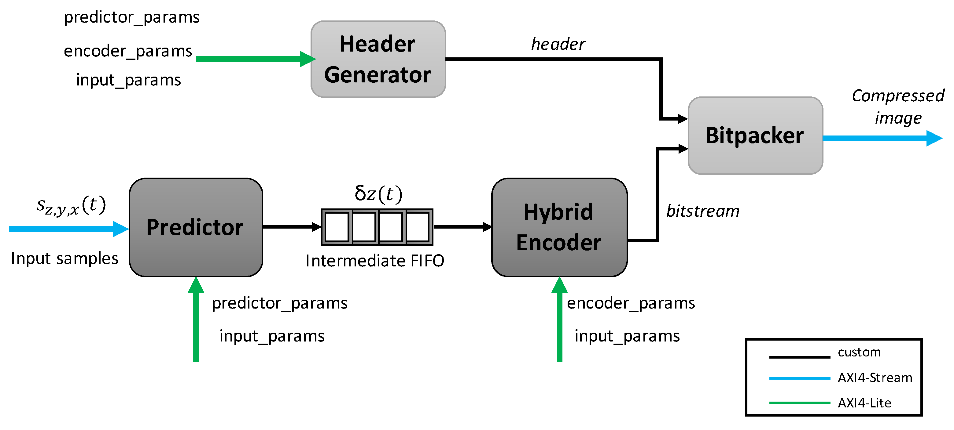
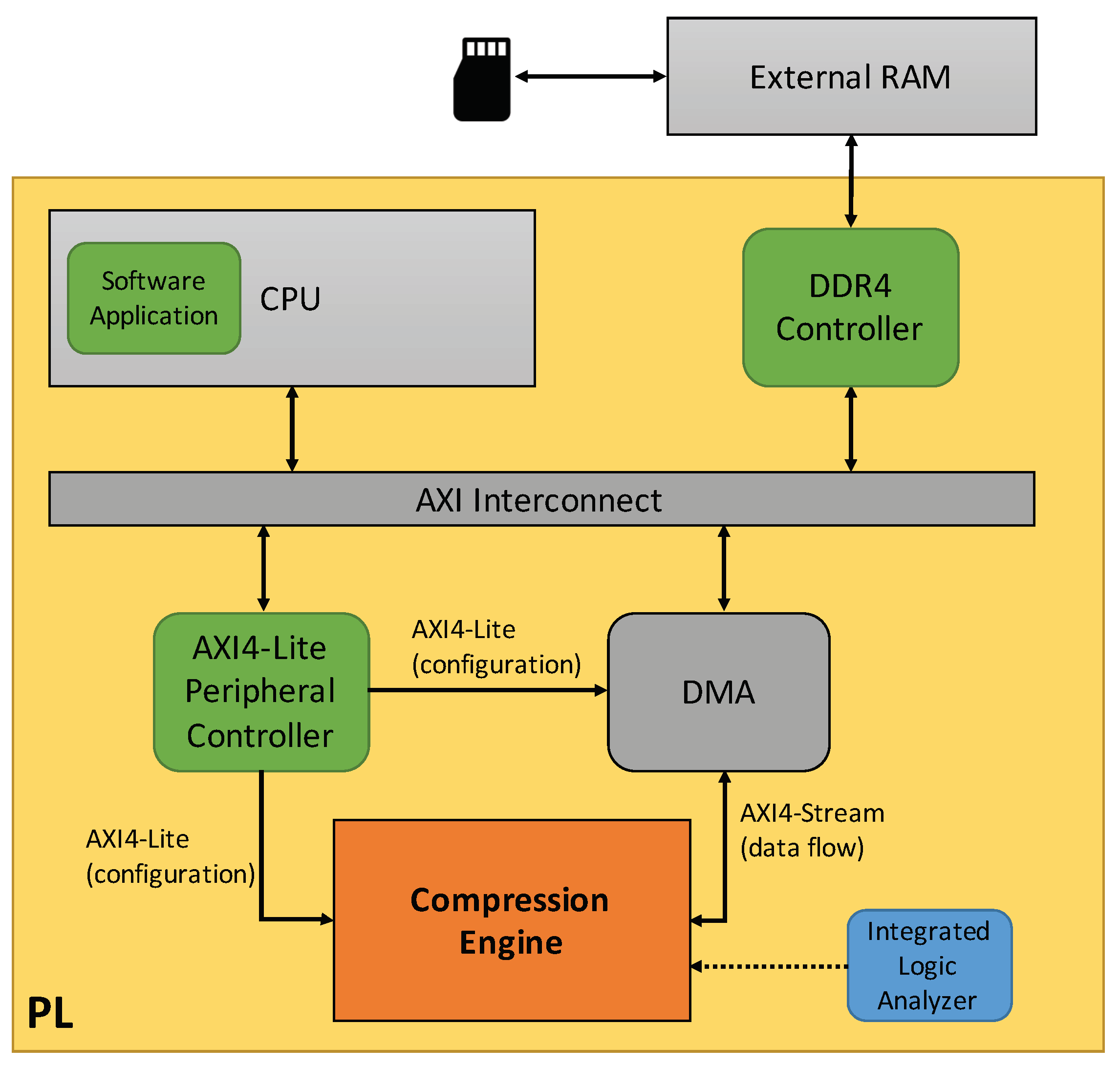
3. Hardware Design

The presented solution has been developed by using an HLS methodology. Concretely, the recent Xilinx Vitis HLS tool (v2020.2) has been employed to model the algorithm behavior in C/C++ for obtaining the equivalent VHDL description that forms the final IP core, since this tool provides optimized HLS solutions for Xilinx FPGA devices. The HLS model was conceived from the beginning of its development keeping in mind limitations regarding synthesizable C/C++ constructions (e.g., memory allocations, careful use of pointers, etc.), just requiring some optimizations in the memory accesses after an initial debugging. The focus of the implementation is to obtain a reduced initiation interval at the cost of a moderate hardware occupancy, taking advantage of the low-complexity nature of the algorithm. For this reason, we force the HLS tool to obtain the lowest initiation interval by applying the pipeline pragma at the task level, taking into account data dependencies between sub-stages. Bit-accurate data types have been used to develop the different functional modules instead of standard C/C++ data types, allowing in this case to reduce logic resources’ consumption.

The design processes the hyperspectral images in the Band Interleaved by Line (BIL) order, which is used by push broom sensors, obtaining a line of samples in the spatial domain for all the spectral channels before acquiring the next one. The different modules have been developed following a dataflow-oriented strategy, managing an image sample each time and allowing in this way to pipeline the processing of consecutive samples. A global overview of the whole design is shown in Figure 3, including the different interfaces used for configuration and interconnection among modules. In addition to the main compression chain, comprised by the predictor and the hybrid encoder, two extra modules are included: the header generator, which creates the necessary fields to allow a correct decompression, parallel to the compression datapath; and the bitpacker, which takes the output of both the header generator and the hybrid entropy coder to form the output bitstream, including the encoder image tail.

3.1. Predictor

The predictor includes all the necessary units to generate a mapped prediction residual ${\delta }_z\left(t\right)$ from a given input sample $s_{z,y,x}$. The top-level module receives the user-defined predictor parameters, together with the image size and the dynamic range D through an AXI4-Lite interface in compile time, providing an interface that is suitable for configuration ports that work at low data rates. This configuration can be changed also in run-time, but the IP operation should stop between consecutive compressions until the new configuration is written in the defined AXI4-Lite configuration registers. Input samples are received by using a lightweight AXI4-Stream interface, a communication protocol which is intended for burst transfers at high data rates, including also a simple handshaking protocol for synchronization purposes, comprised by a VALID and READY signals. At the output, mapped prediction residuals ${\delta }_z\left(t\right)$ are stored in an intermediate FIFO, which then feeds the hybrid encoder.

The internal processing is done by a total of nine units, as shown in Figure 4. Two memories are created at the top level, which are then used by the different submodules: topSamples, which stores the previous spectral line ($N_x·N_z$ samples), needed to perform both the local sum and the directional local differences (if the full prediction mode is selected); and currentSamples, responsible for storing $N_x·P$ samples to compute the central local differences. Thus, as long as the image is being processed, samples which are not needed anymore to calculate the central local differences because they fall more than P bands behind the sample being currently processed are moved from currentSamples to topSamples. In the same way, samples in topSamples are replaced each time a spectral line is fully predicted, prior to start the processing of the next line. The sample at the same position as the current one but in the previous band ($s_{z-1,y,x}$) is also stored in a register, since it is used to calculate the double-resolution predicted sample ${\tilde{s}}_z\left(t\right)$.

First of all, previously preprocessed samples, which are stored in currentSamples and topSamples, and the current one are ordered in five FIFOs in the Read_samples module, corresponding to the current position and the vicinity needed to perform both the local sum and the directional local differences (i.e., samples at the left, top-left, top and top-right positions). These FIFOs have a depth of $P+1$.

Then, both the local sum and the local differences are computed in the Compute_differences module. The selection of the local sum and prediction mode is defined at compile-time by user-defined parameters. The local differences are calculated simultaneously in a single clock cycle independently of the selected prediction mode, since there are not data dependencies.

Once the local differences vector $U_z\left(t\right)$ is available, the predicted local difference ${\widehat{d}}_z\left(t\right)$ is computed as the inner product between $U_z\left(t\right)$ and the weight vector $W_z\left(t\right)$. After that, all the components to calculate the high-resolution predicted sample are available, obtaining ${\breve{s}}_z\left(t\right)$ in the High_resolution_prediction unit. The result of this operation is truncated taking into account the value of the register size R, though this calculation can be omitted if it is guaranteed that the size of the operation result never exceeds R.

Taking ${\breve{s}}_z\left(t\right)$ as input, the double-resolution predicted sample ${\tilde{s}}_z\left(t\right)$ is calculated in the Prediction module, using a right shift operation to implement the division by a power of two. The predicted sample is immediately obtained applying the Formula (10). Finally, the output of this unit is the prediction residual, which is calculated as

$${\Delta }_z\left(t\right)=s_{z,y,x}-{\widehat{s}}_{z,y,x}.$$

(21)

As this submodule only employs basic arithmetic and logic operations, its process takes a single clock cycle.

If $m_z\left(t\right)\ne 0$ (i.e., near-lossless compression), the next step in the processing chain is the Quantizer unit; otherwise, it is bypassed. This module is a critical point in the datapath, since it makes use of a division that it is not efficiently implemented by HLS tools, considerably delaying the latency. In the proposed solution, a new approach is presented, substituting the division by a multiplication by the inverse of the division, operation that is highly optimized by using the internal DSPs of the FPGA. For this purpose, a Look-Up Table (LUT) is previously defined with the result of the division $\frac{1}{X}$ in a fixed-point (i.e., integer precision), X being the different divisor values in the range of error limits defined by the target application. The required LUT size would be of $2^{D_a}-1$ words if only absolute errors are used, $2^{D_r}-1$ words if only relative errors are used, and the minimum of both values if both error types are used. To avoid rounding issues for certain divisors, the computation of the inverse values of denominator is done in excess. Following this strategy also in the divisions performed in the Mapper, the responsibility of generating the unsigned mapped residuals ${\delta }_z\left(t\right)$, a reduction of around the 30% of the predictor latency, is observed, compared with the version that implements directly the division.

The Quantizer_bin_center and the Local_decompressor units are responsible for performing the sample reconstruction, in order to properly estimate the value of the sample representative $s_{z,y,x}^{″}$, used during the processing of the next image samples. While the first calculates the bin center $s_z^{\prime }\left(t\right)$ in one clock cycle, as indicated in Equation (15), the latter estimates the value of $s_{z,y,x}^{″}$ only if the user-defined parameter $\mathsf{\Theta }\ne 0$; otherwise, $s_{z,y,x}^{″}=s_{z,y,x}$. The calculation of the sample representative value is optimized for a hardware implementation, substituting power-of-two operations and the division reflected in Equation (16) by logical shifts. Since the rest of parameters used for the calculation are previously known, including the sign of the quantized index $q_z\left(t\right)$, this step is also executed in only one clock cycle.

Finally, the prediction chain is closed with the Compute_weights module, which performs both the weights initialization or their update, depending on the current image coordinates. The latency of the weight update directly depends on the selected prediction mode, which defines the number of components in the weights vector. However, this process is done simultaneously for the different weight components, since there are not data dependencies among them. In addition, the proposed solution takes into account data dependencies with adjacent samples during the weight update when the compression is done in BIL order, trying to reduce the impact of those dependencies in the global throughput. An extra memory is defined in the design, denoted as FullWeights, whose size is $N_z·C_z$ and which is used to store the state of the weights vector at each band z, recovered then to process the next image pixel in the same band.

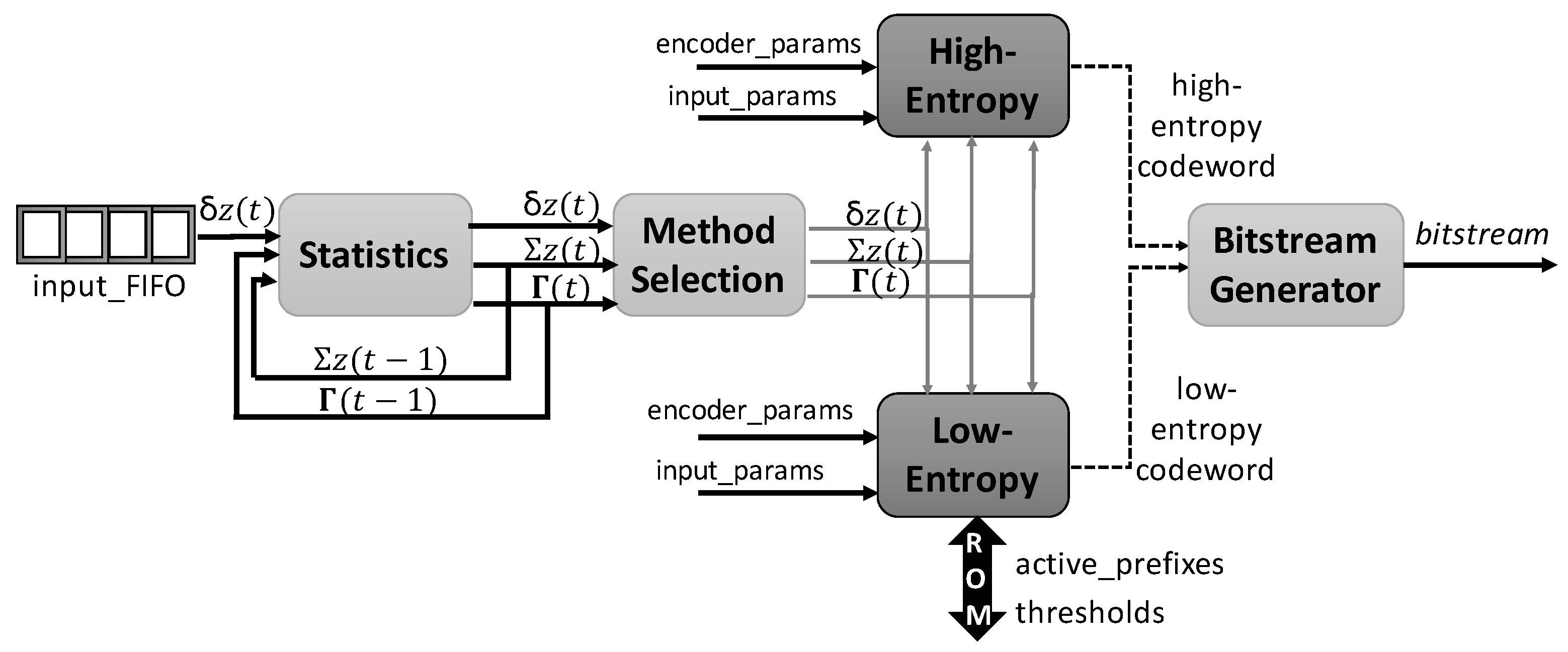
3.2. Hybrid Encoder

This module receives the encoder parameters, the image size, and the pixel resolution D through an AXI4-Lite interface. Then, the input samples are received from the intermediate FIFO, where the predictor writes the prediction residuals $\delta \left(t\right)$ as soon as they are generated. The output interface is based on a basic AXI4-Stream interface that uses the VALID and READY signals for dataflow control (i.e., a simple handshaking protocol), in addition to the LAST signal that indicates the transmission of the last codeword. The variable-length codes (a single codeword for each high-entropy code or a codeword comprised by multiple low-entropy codes) are sent grouped in words of $W\_BUFFER$ bytes, a parameter defined by the user. An extra flag, named End-of-Processing (EOP), is used to inform the Bitpacker that the encoder has finished generating the bitstream. In addition, both the final state of the 16 low-entropy codes and the accumulator values for each band z are saved in FIFOs, which are accessed by the Bitpacker in order to properly generate the image tail.

The top-level block diagram of the hybrid encoder is shown in Figure 5, which is comprised of four modules: the Statistics module, the responsibility for initializing, updating and rescaling both the counter and the accumulator; the Method Selection unit that implements Equation (18) and consequently decides which encoding method is selected; and the Bitstream Generator, which solves the bottleneck of outputting the resultant codeword generated by the hybrid encoder in a bit-by-bit manner (it being possible to complete more than one byte in the same iteration or even leave an incomplete byte), thus adapting data rates; and the two main modules that compute the high- and low-entropy methods, as described below.

3.2.1. High-Entropy

This unit is responsible for encoding the mapped residual $\delta \left(t\right)$ using a high-entropy codeword, when Equation (18) is satisfied. This process employs RLL-GPO2 codes, for which the procedure is based on the next assumptions:

1

If $\delta \left(t\right)/2^k<U_{max}$, the codeword is comprised of the k least significant bits of $\delta \left(t\right)$, followed by a one and $\delta \left(t\right)/2^k$ zeros. The parameter k is known as code index.

2

Otherwise, the high-entropy codeword consists of the representation of $\delta \left(t\right)$ with D bits, with D being the dynamic range of each input pixel, followed by $U_{max}$ zeros.

The high-entropy module is divided into two main parts: the computation of the k value and the writing of the resultant codeword in the output bitstream. The calculation of k has been done in an iterative way, accelerated by following a pipelining strategy and avoiding the use of complex arithmetic operations, such as divisions, which are not fully optimized by HLS tools.

3.2.2. Low-Entropy

This module encodes the mapped residual $\delta \left(t\right)$ when Equation (18) is not satisfied. For doing so, the mapped residuals are set into one of the 16 group of values identified by a code index, i. The management of the input-to-output and flush input-to-output codeword tables in hardware result in computationally inefficient hardware, if the process is implemented as described in the standard. To overcome this issue, the information present in these tables, as well as the searching patterns, have been reorganized. For doing so, the information present in the input-to-output codeword table for each code index, i, and its corresponding flush input-to-output codeword table have been merged into two arrays, named ${\mathrm{APl}}_i$ and ${\mathrm{APv}}_i$. Additionally, the corresponding ${\mathrm{AP}}_i$ is implemented as an index used to move inside ${\mathrm{APl}}_i$ and ${\mathrm{APv}}_i$ arrays (i.e., as an offset), and hence, it is initialized as 0 instead to a null sequence. For each $\delta \left(t\right)$, in this new version, the $l_z\left(t\right)$ is calculated as

$$l_z\left(t\right)=min(\delta \left(t\right),L_i+1).$$

(22)

As described in the standard, if $\delta \left(t\right)$ exceeds $L_i$, the residual value $\delta \left(t\right)-L_i-1$ is directly encoded to the bitstream as it is done in the high-entropy mode, with a k value equal to 0. After calculating $l_z\left(t\right)$, ${\mathrm{AP}}_i$ is updated as

$${\mathrm{AP}}_i={\mathrm{AP}}_i+l_z\left(t\right)+1.$$

(23)

Then, l and v are obtained as ${\mathrm{APl}}_i\left({\mathrm{AP}}_i\right)$ and ${\mathrm{APv}}_i\left({\mathrm{AP}}_i\right)$, respectively. Two actions can be carried out depending on the l value:

1

If l value is not 0, v value is written to the bitstream using l bits and ${\mathrm{AP}}_i$ is reset to 0.

2

If l value is equal to 0, ${\mathrm{AP}}_i$ is updated to v value (${\mathrm{AP}}_i=v$).

After processing all the $\delta \left(t\right)$ values, the remaining active prefixes are added to the bistream by directly coding the current ${\mathrm{APv}}_i\left({\mathrm{AP}}_i\right)$ values using ${\mathrm{APl}}_i\left({\mathrm{AP}}_i\right)$ bits. Following this simple strategy, the number of memory accesses and operations needed to process and update the active prefixes, and to obtain the output codewords according to the input ones is strongly optimized.

3.3. Header Generator

This unit is responsible for generating the appropriate header fields to allow a correct decompression of the generated bitstream. The length of this header directly depends on the compression configuration. Image, predictor, and encoder parameters are sent to this module through an AXI4-Lite interface, while the generated header is sent through a lightweight AXI4-Stream interface to the Bitpacker. The performance of this module is done in parallel to the main compression datapath, since its behavior is essentially sequential and compensating in this way the global latency of the system.

3.4. Bitpacker

The last step of the compression chain is the Bitpacker, which takes the output of both the Header Generator and the Hybrid Encoder modules to generate the compressed image, formed by the header, the codewords, and the image tail, created also in this module. The unit has two input data interfaces, one to receive the header coming from the Header Generator and the other through it receives the bitstream from the Hybrid Encoder. Both input interfaces, implemented with AXI4-Stream interfaces, include the necessary control signals for dataflow management. Taking into account the value of the VALID signals of both input interfaces, the IP is able to identify if it should be ready to receive a header or a bitstream, appending it correctly at the output interface, also implemented with an AXI4-Stream interface. When the EOP flag generated by the Hybrid Encoder is asserted, the Bitpacker recognizes that both the header and the bitstream have been received, and it is time to generate the image tail, as it is indicated by the standard. For this purpose, it accesses the two FIFOs where the final state of both the 16 low-entropy codes and the accumulator values for each band z have been stored.

4. Experimental Results

The proposed solution has been initially verified by simulation during the different development stages (i.e., algorithmic, post-HLS, and post-synthesis levels), in order to ensure its correct behavior once it is mapped on hardware. A software model has been used as golden reference, comparing bit by bit the output of the hardware solution for each one of the tests performed with the results provided by that golden reference. A total of 124 tests have been performed by combining seven different images, including AVIRIS scenes and synthetic images to debug corner cases, with multiple configuration sets, ensuring that at least the different local sum and prediction options are covered in both lossless and near-lossless modes. In the latter case, both absolute and relative errors were used, in band-dependent and band-independent modes.

Then, the proposed compression solution has been mapped on a Xilinx KCU105 development board, which includes a Kintex UltraScale FPGA (XCKU040-2FFVA1156E). The baseline configuration is summarized in

Table 2. Main configuration parameters of the CCSDS 123.0-B-2 proposed solution used for synthesis purposes.

Parameter	Value
Image parameters
Columns, $N_x$	677
Lines, $N_y$	512
Bands, $N_z$	224
Dynamic Range, D	16
Encoding Order	BIL
Predictor parameters
Bands for Prediction, P	3
Local Sum Mode	Narrow Neighbour-Oriented
Prediction Mode	Full Prediction
Weight Resolution, $\mathsf{\Omega }$	16
Sample Adaptive Resolution, $\mathsf{\Theta }$	2
Sample Adaptive Offset, ${\psi }_z$	1
Sample Adaptive Damping, ${\varphi }_z$	1
Error Method	Absolute
Absolute Error Bitdepth, $D_a$	8
Absolute Error Value, $A_z$	4
Encoder parameters
Unary Length Limit, $U_{max}$	16
Rescaling Counter Size, $\gamma \ast$	5
Initial Count Exponent, ${\gamma }_0$	1

, restricting supported image dimensions to the ones of the AVIRIS scenes, since they are the ones used for validation purposes. The value of D is also fixed to target the AVIRIS sensor. The rest of the parameter values have been selected after an exhaustive parameter tuning on software, where up to 15,000 tests were launched to find the configuration that achieves best results in terms of compression performance under lossless mode. Therefore, the absolute error value can be modified, depending on the target application.

Area consumption of the whole compression chain is summarized in

Table 3. Resource utilization of the CCSDS 123.0-B-2 compressor on Xilinx Kintex UltraScale XCKU040.

	36 Kb BRAM	DSP48E	Registers	LUTs
Predictor	76 (12.7%)	54 (2.8%)	6054 (1.3%)	10,087 (4.1%)
Hybrid Encoder	9 (1.5%)	9 (0.5%)	2498 (0.5%)	4286 (1.8%)
Header generator	0 (0%)	0 (0%)	2976 (0.6%)	2478 (1.0%)
Bitpacker	0 (0%)	0 (0%)	387 (0.1%)	334 (0.1%)
Total	85 (14.2%)	63 (3.3%)	11,915 (2.5%)	17,185 (7.0%)

, specifying the resources utilization of each stage. As it can be observed, the predictor is the critical module in terms of both memory and logic resources usage, consuming the 12.7% of BRAMs and the 4.1% of LUTs available in the target device. These results were expected, since the prediction stage is the one that performs more complex operations, such as the modified divisions performing under near-lossless compression in the feedback loop. The consumption of DSPs supposes around the 3.3% of the total available in the device. These resources are mainly used to perform the different multiplications present in the design, such as the the multiplication by the precomputed inverse performed in both the quantizer and the mapper, and the dot product between the local differences vector $U_{z,y,x}$ and the weights vector $W_{z,y,x}$, both performed in the prediction stage; or to compute Equations (18) and (19), calculated under the low-entropy mode in the hybrid encoder. It is remarkable that the storage usage of this module is directly proportional to the image size, since the more restrictive memory is topSamples and, as it was mentioned in Section 3.1, its dimension depends on $N_x$ and $N_z$ values. Anyway, the configuration used for this experiment targets AVIRIS, which provides a scene large enough in both the spatial and the spectral domain to characterize the compression solution, fitting well in an equivalent FPGA in terms of logic resources to the recent space-qualified Xilinx Kintex UltraScale XQRKU060 device. In addition, the target device still has enough logic and memory resources available to target high hyper- and ultraspectral scenes or to include additional functionality to the compression chain in the space payload.

All the modules that conform the compression chain have been successfully synthesized with a targeted maximum clock frequency of 125 MHz, the maximum reached by the predictor, which is the limiting stage.

In addition to the compression chain explained in Section 3, the test-setup is completed with a MicroBlaze embedded microprocessor, part of the Xilinx IP catalog, to manage IP initialization and test behavior, the necessary AXI infrastructure to interconnect the different modules and a Direct Memory Access (DMA) unit, which handles data transactions between the compression chain and the off-chip memory, where the input image is located prior to starting the tests. The access to that external memory is done through a dedicated DDR4 memory controller. These transactions are transparent for the CPU, working in its main thread without requiring its intervention for data transfers. Input images are loaded into the external RAM from an SD card, by using the Xilinx xilffs library, which runs into the MicroBlaze soft processor and provides the necessary software functions to interact with that storage device. A specific AXI module is also used to manage module initialization and configuration through AXI4-Lite interfaces. Integrated Logic Analyzers (ILAs) are also integrated as part of the set-up during the on-chip debugging stage, monitoring the different I/Os of the developed compression chain to validate its correct behavior. An overview of the whole test set-up is shown in Figure 6. The inclusion of these modules in the design implies a resources utilization overhead of 15% of LUTs, 9% of registers, and 13% of dedicated memory, compared to the area consumed by the whole compression chain, previously summarized in Table 3. On the other side, DSP usage remains constant.

The whole validation set-up also runs at a clock frequency of 125 MHz, except the DDR4 controller, which is fed with a dedicated clock at 300 MHz for high-speed access to the off-chip memory. The bottleneck of the processing chain is the predictor, due to the feedback loop implemented to support near-lossless compression, generating a prediction residual $\delta \left(t\right)$ every seven clock cycles. The other modules have a latency of one clock cycle including the hybrid encoder, since it always selects the high-entropy method when AVIRIS scenes are compressed; otherwise, its latency will be variable, depending on the number of samples that are coded by using the low-entropy technique. The latency of the header generator, which has a sequential behavior, is overlapped with the rest of the compression solution by executing both processes simultaneously. Therefore, the latency of the whole compression chain is 13 clock cycles to fully process an input sample. Taking into account that the presented solution has a linear behavior, the throughput of the system is imposed by the predictor, and it can be calculated as following the reflected, considering a sample of a 16-bit input pixel of an AVIRIS scene

$$Throughput=\frac{1}{T_{predictor}·\frac{1}{f}}=\frac{1}{7·\frac{1}{125·{10}^6}}=17.86(MSamples/s),$$

(24)

with $T_{predictor}$ being the number of clock cycles taken by the predictor to generate a mapped residual $\delta \left(t\right)$ and f the system clock frequency, fixed to 125 MHz.

Although this throughput could prevent the use of this solution in real-time applications, it can be easily improved by placing multiple instances of the compression chain in parallel, since there is enough margin in terms of resources utilization, as reflected in Table 3. The proposed strategy is based on compressing N image portions simultaneously, by using N compression engines working in parallel. This mechanism is also robust against radiation effects, since an error in one image segment implies that it is lost but not the rest of the image, which can be recovered during the decompression. Although this scheme increases the system complexity, since it requires a splitter at the beginning of the compression chain, which would be responsible for dividing the image into portions and sending them to the different compression engines, it is considered acceptable taking into account the logic resources available in the target device. This scheme has been successfully evaluated in [22], obtaining different results in terms of compression performance and reconstructed image quality, depending on the partitioning pattern. The compression ratio can be affected if intermediate statistics (e.g., sample vicinity used during the prediction or the weight vectors) are not shared among compression engines, but it would be needed to achieve a trade-off between losses in the compression ratio and the architectural complexity that implies to share those statistics among instances.

Regarding the power consumption, the Vivado tool reports a total of 2.48 W, with 1.98 W being the derived from the developed implementation (i.e., device dynamic consumption) and the remaining 0.5 W the device static consumption, which represents the transistor leakage power just for powering the device. The more consuming resources are the interface with the external DDR4 memory (0.844 W, the 42% of total dynamic consumption), and the clock generation and distribution (0.742 W, 37% of the total).

Finally,

Table 4. Comparison between CCSDS-123 VHDL and HLS implementations.

Implementation	Development Time (Months)	Encoder	LUTs	FFs	DSPs	BRAMs	Freq. (MHz)	Throughput (MSamples/s)
SHyLoC 2.0 [16]	24	Sample	5975	3599	13	74	152	59.4
This work	6	Hybrid	17,185	11,915	63	85	125	17.86

shows a comparison between the presented work and a previous FPGA implementation of the CCSDS 123.0-B-1 compression standard, which only supports lossless compression, fully developed in VHDL [16]. Although the VHDL implementation and the results of the solution presented in [16] are provided for the Band-Interleaved by Pixel (BIP) order, the one that is able to achieve the processing of one sample per clock cycle, results for the BIL order are used in this comparison, for a more realistic comparison with the approach presented in this work. As it can be observed, there is an increment in the logic resources utilization due to the introduction of the quantization feedback loop in the presented approach, to be able to compress in near-lossless mode. The use of the new hybrid encoder instead of the sample-adaptive one described in Issue 1 of the standard also implies a higher logic resources usage. This is added to the fact that generally HLS implementations are not capable of mapping the developed model in the available resources in an optimal way, as it is done in an RTL description. This area overhead is around +188% of LUTs and +15% of BRAMs. The high amount of difference in the use of DSPs, around +79%, is derived from the quantizer inclusion, which uses multiplications, this being the resource that performs these arithmetic operations. In addition, both architectural modifications also imply a reduction of −70% in terms of throughput. The main strength of the presented work is the development time thanks to using an HLS design methodology, obtaining a functional model +75% faster (i.e., in less time) than following an RTL strategy. In this way, the benefits of HLS are demonstrated to provide a behavioral description of the final system that, though it does not reach a fully optimized model in terms of area utilization and timing constraints, it serves as a starting point for prototyping purposes. It is intended that future FPGA implementations of the CCSDS 123.0-B-2 near-lossless compression standard takes the presented approach as the worst case, since it is expected that VHDL descriptions always obtain better results in terms of resources usage and throughput than one developed following an HLS design strategy.

5. Conclusions

In this work, a hardware implementation of the 123.0-B-2 compression standard from the CCSDS has been presented, which was accomplished following an HLS design methodology. This standard is conceived for the lossless to near-lossless compression of multi- and hyperspectral images, featuring a reduced computational complexity which is well suited for space missions. From an architectural point of view, the design has been partitioned in several components (predictor, hybrid encoder, header generator, and bitpacker) interconnected through AXI communication buses. These units have been designed using a dataflow-oriented strategy, thus allowing a pipelined operation. In addition, several optimizations have been adopted in order to improve processing performance, such as the implementation of division operations as multiplications or the reformulation of low entropy coding tables, among others. The whole design has been designed using the recent Xilinx Vitis HLS tool, and implemented and validated on a Xilinx Kintex UltraScale XCKU040 FPGA. Resource utilization of 7% of LUTs and around 14% of BRAMs has been reported, with a processing performance of 12.5 MSamples/s and a reduced power consumption. These results demonstrate the viability of this solution for on-board multi- and hyperspectral image compression even for real-time applications, if multiple compression instances work in parallel. In this way, we present, to the best of our knowledge, the first fully-compliant hardware implementation of the CCSDS 123.0-B-2 near-lossless compression standard available in the state-of-the-art.

The next steps are focused on optimizing the predictor latency by a hand-made VHDL description to enhance the throughput of the whole compression solution, since it is the main bottleneck of the implementation. In addition, the implementation of Single Event Effect (SEE) mitigation techniques, such as hardware redundancy or EDAC mechanisms to detect and correct errors in the internal memory, will be evaluated, in order to provide to the design robustness against radiation effects on on-board electronics.

References

- Qian, S.E. Introduction to Hyperspectral Satellites. In Hyperspectral Satellites and System Design; CRC Press, Taylor & Francis Group: Abingdon, UK, 2020; Chapter 1; pp. 1–52. [Google Scholar]
- Benediktsson, J.A.; Chanussot, J.; Moon, W.M. Very High-Resolution Remote Sensing: Challenges and Opportunities [Point of View]. Proc. IEEE 2012, 100, 1907–1910. [Google Scholar] [CrossRef]
- Fu, W.; Ma, J.; Chen, P.; Chen, F. Remote Sensing Satellites for Digital Earth. In Manual of Digital Earth; Guo, H., Goodchild, M.F., Annoni, A., Eds.; Springer: Singapore, 2020; pp. 55–123. [Google Scholar] [CrossRef] [Green Version]
- Montealegre, N.; Merodio, D.; Fernández, A.; Armbruster, P. In-flight reconfigurable FPGA-based space systems. In Proceedings of the 2015 NASA/ESA Conference on Adaptive Hardware and Systems (AHS), Montreal, QC, Canada, 15–18 June 2015; pp. 1–8. [Google Scholar] [CrossRef]
- Boada Gardenyes, R. Trends and Patterns in ASIC and FPGA Use in Space Missions and Impact in Technology Roadmaps of the European Space Agency. Ph.D. Thesis, UPC, Escola Tècnica Superior d’Enginyeria Industrial de Barcelona, Barcelona, Spain, 2011. [Google Scholar]
- Habinc, S. Suitability of Reprogrammable FPGAs in Space Applications. Gaisler Research. 2002. Available online: http://microelectronics.esa.int/techno/fpga_002_01-0-4.pdf (accessed on 2 September 2021).
- Coussy, P.; Gajski, D.D.; Meredith, M.; Takach, A. An Introduction to High-Level Synthesis. IEEE Des. Test Comput. 2009, 26, 8–17. [Google Scholar] [CrossRef]
- Cong, J.; Liu, B.; Neuendorffer, S.; Noguera, J.; Vissers, K.; Zhang, Z. High-Level Synthesis for FPGAs: From Prototyping to Deployment. IEEE Trans. -Comput.-Aided Des. Integr. Circuits Syst. 2011, 30, 473–491. [Google Scholar] [CrossRef] [Green Version]
- Consultative Committee for Space Data Systems. Low-Complexity Lossless and Near-Lossless Multispectral and Hyperspectral Image Compression, CCSDS 123.0-B-2; CCSDS: Washington, DC, USA, 2019; Volume 2. [Google Scholar]
- Blanes, I.; Kiely, A.; Hernández-Cabronero, M.; Serra-Sagristà, J. Performance Impact of Parameter Tuning on the CCSDS-123.0-B-2 Low-Complexity Lossless and Near-Lossless Multispectral and Hyperspectral Image Compression Standard. Remote Sens. 2019, 11, 1390. [Google Scholar] [CrossRef] [Green Version]
- Hernandez-Cabronero, M.; Kiely, A.B.; Klimesh, M.; Blanes, I.; Ligo, J.; Magli, E.; Serra-Sagrista, J. The CCSDS 123.0-B-2 Low-Complexity Lossless and Near-Lossless Multispectral and Hyperspectral Image Compression Standard: A comprehensive review. IEEE Geosci. Remote Sens. Mag. 2021, in press. [Google Scholar] [CrossRef]
- Barrios, Y.; Rodríguez, P.; Sánchez, A.; González, M.; Berrojo, L.; Sarmiento, R. Implementation of cloud detection and processing algorithms and CCSDS-compliant hyperspectral image compression for CHIME mission. In Proceedings of the 7th International Workshop on On-Board Payload Data Compression (OBPDC), Online Event, 21–23 September 2020; pp. 1–8. [Google Scholar]
- Chatziantoniou, P.; Tsigkanos, A.; Kranitis, N. A high-performance RTL implementation of the CCSDS-123.0-B-2 hybrid entropy coder on a space-grade SRAM FPGA. In Proceedings of the 7th International Workshop on On-Board Payload Data Compression (OBPDC), Online Event, 21–23 September 2020; pp. 1–8. [Google Scholar]
- Consultative Committee for Space Data Systems. Lossless Multispectral and Hyperspectral Image Compression, Recommended Standard CCSDS 123.0-B-1; CCSDS: Washington, DC, USA, 2012; Volume 1. [Google Scholar]
- Santos, L.; Gomez, A.; Sarmiento, R. Implementation of CCSDS Standards for Lossless Multispectral and Hyperspectral Satellite Image Compression. IEEE Trans. Aerosp. Electron. Syst. 2019, 56, 1120–1138. [Google Scholar] [CrossRef]
- Barrios, Y.; Sánchez, A.; Santos, L.; Sarmiento, R. SHyLoC 2.0: A versatile hardware solution for on-board data and hyperspectral image compression on future space missions. IEEE Access 2020, 8, 54269–54287. [Google Scholar] [CrossRef]
- Tsigkanos, A.; Kranitis, N.; Theodorou, G.A.; Paschalis, A. A 3.3 Gbps CCSDS 123.0-B-1 multispectral & Hyperspectral image compression hardware accelerator on a space-grade SRAM FPGA. IEEE Trans. Emerg. Top. Comput. 2018, 9, 90–103. [Google Scholar]
- Fjeldtvedt, J.; Orlandic, M.; Johansen, T.A. An Efficient Real-Time FPGA Implementation of the CCSDS-123 Compression Standard for Hyperspectral Images. IEEE J. Sel. Top. Appl. Earth Obs. Remote Sens. 2018, 11, 3841–3852. [Google Scholar] [CrossRef] [Green Version]
- Bascones, D.; Gonzalez, C.; Mozos, D. FPGA Implementation of the CCSDS 1.2.3 Standard for Real-Time Hyperspectral Lossless Compression. IEEE J. Sel. Top. Appl. Earth Obs. Remote Sens. 2018, 11, 1158–1165. [Google Scholar] [CrossRef]
- Orlandic, M.; Fjeldtvedt, J.; Johansen, T.A. A Parallel FPGA Implementation of the CCSDS-123 Compression Algorithm. Remote Sens. 2019, 11, 673. [Google Scholar] [CrossRef] [Green Version]
- Bascones, D.; Gonzalez, C.; Mozos, D. Parallel Implementation of the CCSDS 1.2.3 Standard for Hyperspectral Lossless Compression. Remote Sens. 2017, 9, 973. [Google Scholar] [CrossRef] [Green Version]
- Barrios, Y.; Rodríguez, A.; Sánchez, A.; Pérez, A.; López, S.; Otero, A.; de la Torre, E.; Sarmiento, R. Lossy Hyperspectral Image Compression on a Reconfigurable and Fault-Tolerant FPGA-Based Adaptive Computing Platform. Electronics 2020, 9, 1576. [Google Scholar] [CrossRef]