Abstract
Self-supervised method has proven to be a suitable approach for despeckling on synthetic aperture radar (SAR) images. However, most self-supervised despeckling methods are trained by noisy-noisy image pairs, which are constructed by using natural images with simulated speckle noise, time-series real-world SAR images or generative adversarial network, limiting the practicability of these methods in real-world SAR images. Therefore, in this paper, a novel self-supervised despeckling algorithm with an enhanced U-Net is proposed for real-world SAR images. Firstly, unlike previous self-supervised despeckling works, the noisy-noisy image pairs are generated from real-word SAR images through a novel generation training pairs module, which makes it possible to train deep convolutional neural networks using real-world SAR images. Secondly, an enhanced U-Net is designed to improve the feature extraction and fusion capabilities of the network. Thirdly, a self-supervised training loss function with a regularization loss is proposed to address the difference of target pixel values between neighbors on the original SAR images. Finally, visual and quantitative experiments on simulated and real-world SAR images show that the proposed algorithm notably removes speckle noise with better preserving features, which exceed several state-of-the-art despeckling methods.
1. Introduction
Synthetic aperture radar (SAR) [1] is an active remote sensing imaging sensor that transmits electromagnetic signals to target in a slant distance manner. Compared with optical imaging sensors, SAR has the imaging ability of all-time and all-weather. Therefore, SAR has become one of the remote sensors used for disaster assessment [2], resource exploration [3], ocean surveillance [4,5] and statistical analysis [6]. Nevertheless, due to the imaging mechanism, the quality of SAR images is inherently affected by speckle noise [7,8]. Speckle noise is a granular disturbance, usually modeled as a multiplicative noise, that affects SAR images, as well as all coherent images [8]. The speckle noise may severely diminish the performances of detection accuracy [9,10,11,12] and information extraction [13]. Therefore, the reduction of speckle noise is a key and essential processing step for a number of applications.
In the past few decades, numerous researchers have attempted to reduce the speckle noise in SAR images. Generally, the existing despeckling methods can be roughly summarized as local window methods, non-local mean (NLM) methods and deep learning (DL) methods. In the first group, local window methods are widely used, such as Lee [14], Frost [15] and Kuan [16]. The despeckling performance of local window methods is very dependent on the window size. The larger the size, the smoother the despeckled image and the better the despeckling performance. However, the despeckled image will lose point targets, linear features and textures.
To overcome the disadvantage of local window methods, NLM methods are applied to process SAR images, such as PPB [17], SAR-BM3D [18] and NL-SAR [19]. The NLM methods define the similar pixel and pixel weight by measuring the similarity between a local patch centered on the reference pixel and another local patch centered on a selected non-local neighborhood pixel. The greater the similarity, the larger the weight. However, the NLM methods need to use the equivalent number of looks (ENL) as a prior. In practical applications, it is impossible to obtain the accurate ENL of SAR images. In addition, the time complexity of the local window methods and NLM methods is very high.
Recently, benefiting from new breakthroughs of deep learning [20,21], more and more researchers began to explore DL methods [22,23,24,25,26,27,28,29,30,31,32,33]. The essence of the DL despeckling methods is to learn a relationship from noisy SAR images to noise-free SAR images. It can be described as follows. Firstly, the input of the DL despeckling methods is a noisy SAR image. Then, the noisy SAR images are encoded and decoded through convolutional layers, pooling layers, batch normalization layers and activation function layers. Finally, a noise-free SAR image is obtained. According to whether there are clean images as targets, the DL despeckling methods can be distinguished into three broad categories: supervised methods, semi-supervised methods and self-supervised methods.
The supervised despeckling methods [22,23,24,26] use noisy-clean image pairs to train convolutional neural networks (CNNs) and the despeckling models are applied to reduce speckle noise in real-world SAR images. Since there is no noise-free SAR images, the training image pairs of the supervised methods are generated by combining regularization RGB photos (natural images) with simulated speckle noise. The natural images contain camera images [23] and aerial images [24]. The advantage of the generated method is that a large number of noisy-clean image pairs can be easily obtained. A deeper CNN with numerous parameters can be trained. But the disadvantage of the generated method is that it ignores the peculiar characteristics of SAR images. For example, the noise distribution of SAR images is not the same as in natural images, as well as the content, the texture, or the physical meaning of a pixel value [27]. Compared with real-world SAR images, the generated simulated SAR images have quite difference in content and geometry. There are strong scattering points in real-world SAR images, but not in simulated SAR images. Therefore, the despeckling CNNs trained with simulated images will change point targets, linear features and textures in the real-world SAR images. Benefiting from the noise2noise [34] method, semi-supervised methods and self-supervised methods [28,29,30,31] were proposed. The method of noise2noise is to directly use noisy-noisy image pairs to train deep CNNs. The semi-supervised despeckling model [27] used a small number of noisy-clean image pairs to train CNNs. Then, the obtained despeckling model was fine-tuned on the time series real-world SAR images. Fine-tune refers to the despeckling model obtained in the first step for training again using the time series real-world SAR images. Compared with the supervised despeckling methods, the semi-supervised despeckling methods can better reduce the speckle noise from real-world SAR images. Nevertheless, the time series SAR images will have differences at different times, which will limit the despeckling performance. The self-supervised despeckling methods directly use the extensive noisy-noisy image pairs to train CNNs. The noisy-noisy image pairs are generated by using natural images with simulated speckle noises [28], time series SAR images [31] or generative adversarial network (GAN) [35], which still limit the practicability of these methods in real-world SAR images.
Through the above analysis, a simple summary can be made. Firstly, the DL despeckling method is raising great interest. However, most of DL methods are focused on the new networks [22,23,24,25,26,32,33,36], while ignoring the most essential problem. In our opinion, the lack of truely noise-free SAR images is the most essential problem. Simulated SAR images can not really solve this deficiency. Secondly, it can be found that the despeckling CNNs are becoming more and more deeper. Meanwhile, the number of trainable parameters is increasing. The simulated SAR images can be easily generated through the pixel-wise product of clean natural images with simulated speckle noise [30]. When processing real-world SAR images, the despeckling models obtained will bring new challenges. The despeckling CNNs trained with simulated images pairs will change point targets, linear features and textures in the real-world SAR images. Thirdly, although noise2noise method can directly use noisy images as targets, the despeckling performance is still affected by natural images [29] and the performance of GAN [30]. In the previous works [27,28,29,30,31], they can not really use real-world SAR data to train the despeckling CNNs. Therefore, in this paper, inspired by noise2noise [34], a novel self-supervised despeckling algorithm with an enhanced U-Net is proposed. This algorithm is called SSEUNet. Compared with previous despeckling CNNs [27,28,29,30,31], SSEUNet can directly use real-world SAR images for training deep CNNs. The SSEUNet is composed of generation training pairs (GTP) module, enhanced U-Net (EUNet) and a self-supervised training loss function with a regularization loss. The main contributions and innovations of the proposed algorithm are as follows:
- Since the noisy-noisy image pairs generated by [28,30,31] can not be used well in the despeckling task of real-world SAR images, we propose GTP module. GTP module can generate training image pairs from noisy images. It can make it possible to train deep CNNs using real-world SAR images.
- Due to the poor feature extraction and fusion capabilities of U-Net [37], we design a novel deep CNN by enhancing U-Net. The novel deep CNN is called enhanced U-Net (EUNet).
- In order to address the difference of target pixel values between neighbors on the original noisy image, a self-supervised training loss function with a regularization loss is put forward.
- Visual and quantitative experiments conducted on simulated and real-world SAR images show that the proposed algorithm notably reduces speckle noise with better preserving features, which outputform several state-of-art despeckling methods.
The rest of this paper in organized as follows. The related work, which includes noisy-clean despeckling methods and noisy-noisy despeckling methods, are analyzed in Section 2. In Section 3, we detailed describe the proposed methods. Section 4 illustrates the results of visual effect and parameter evaluation metrics. Finally, the conclusions are drawn in Section 5.
2. Related Work
2.1. Noisy-Clean Despeckling Methods
In recent years, benefiting from deep learning, the noisy-clean despeckling methods have been studied in depth. Inspired by denoising CNN [38], Chierchia et al. [22] proposed the first despeckling CNN, which composed of 17 convolutional layers. The training image pairs of SAR-CNN were generated from time series real-world SAR images. The targets were 25-look SAR images. Zhang et al. [24] directly used dilated convolution layers and skip connections to reduce speckle noise from SAR images. The dilated convolution layer allows CNN to have a lightweight structure and small filter size, but the receptive field of the CNN will not be reduced. In addition, skipping connections reduce the problem of vanishing gradients. Similar to SAR-DRN, Gui et al. [25] proposed a dilated densely connections CNN. After considering the bright distribution of the speckle noise, Shen et al. [26] proposed a recursive deep convolutional neural prior model. The model included a data fitting block and a deep CNN prior block. The gradient descent algorithm was used for the data fitting block and the pre-trained dilated residual channel attention network was applied in the deep CNN prior block. Pan et al. [32] combined multi-channel logarithm gaussian denoising (MuLoG) algorithm with a fast and flexible denoising CNN to deal with the multiplicative noise of SAR images. Li et al. [33] designed a CNN with convolutional block attention module to improve representation power and despeckling performance. In order to help the network retain image details, Zhang et al. [39] proposed a multi-connection CNN with wavelet features. Because the NLM method is one of the most promising algorithm, Cozzolino et al. [23] combined NLM method with deep CNN to design a non-local mean CNN (NLM-CNN). The NLM-CNN used deep CNN to provide interpretable results for target pixel and predicted pixel. Mullissa et al. [36] proposed a two-stage despeckling CNN, called deSpeckleNet. The deSpeckleNet sequentially estimated the speckle noise distribution and the noise-free SAR image. Vitale et al. [40] designed a weighted loss function by considering the contents in the SAR images. Except SAR-CNN, the noisy-clean despeckling methods use synthetic training on the simulated SAR images. Due to the differences in imaging mechanisms and image features between SAR and natural images, i.e., grayscale distribution and spatial correlation [41], training on simulated SAR images is not the best solution [30]. Compared with the most advanced traditional despeckling methods, the deep despeckling CNNs have obvious despeckling advantages, but the lack of truly noise-free SAR images is a major limiting factor in despeckling performance.
2.2. Noisy-Noisy Despeckling Methods
In the real-world, it is impossible to obtain noise-free SAR images. Inspired by noise2noise [34], the noisy-noisy despeckling methods [27,28,29,30,31] were studied in depth. Yuan et al. [28] designed a self-supervised densely dilated CNN (BDSS-CNN) for blind despeckling. In the BDSS-CNN, the noisy-noisy image pairs were generated by adding simulated speckle noise with random ENL to natural images. Then, the generated noisy-noisy image pairs were used to train BDSS-CNN. Finally, the obtained despeckling model was applied on the real-world SAR images. Inspired by blind-spot denoising networks [42], Molini et al. [29] reported a self-supervised bayesian despeckling CNN. The training image pairs were constructed from natural images. Yuan et al. [30] designed a practical SAR images despeckling method to reduce the impact of natural images. The method contained two sub-networks. The first sub-network was a GAN, which used to generate the speckle-speckle training paris. The second network was an enhanced nested-UNet, which was trained by using speckle-speckle training paris. It can be found that the quality of the generated speckle images by GAN will directly affect the despeckling performance of the enhanced nested-UNet. Dalsasso et al. [27] and Ma et al. [31] abandoned the methods of using natural images and GAN, they proposed to use time series real-world SAR images. Whilst, the natural landscape often changes significantly at a short period in the time series real-world SAR images. Therefore, the despeckling performance of [27,31] is still limited.
Although noise2noise methods were used to solve the lack of truly noise-free SAR images, the despeckling performance is still affected by nature images [29] and the performance of GAN [30]. In the previous works [27,28,29,30,31], they can not really use real-world SAR images to train the despeckling CNNs. Therefore, we designed a novel self-supervised despeckling algorithm with an enhance U-Net (SSEUNet). The SSEUNet includes a GTP module, an EUNet and a loss function. The GTP module can directly generate training image pairs from real-world noisy images. The generated image pairs are applied to train EUNet through the proposed loss function. When processing real-world SAR images, the proposed SSEUNet can eliminate the influence of natural images, GAN performance and time series images.
3. Proposed Method
In order to train the despeckling CNN directly using real-world SAR images, we propose a novel self-supervised despeckling algorithm, which is called SSEUNet. The SSEUNet is mainly composed of two GTP module, an enhanced U-Net (EUNet) and a loss function. The GTP module is designed to generate noisy-noisy image pairs for training the proposed EUNet. The EUNet is an enhanced version of U-Net, which has stronger feature extraction and fusion capabilities. The loss function is a self-supervised training loss function with a regularization loss, which is applied to optimal EUNet. In this section, Section 3.1 gives an overview of the proposed SSEUNet framework in detail. The detailed implementation of the proposed GTP module is introduced in Section 3.2. The proposed EUNet will be illustrated in Section 3.3. Section 3.4 introduces the loss function of SSEUNet.
3.1. Overview of Proposed SSEUNet
The proposed SSEUNet is composed of generation training pairs (GTP) module, enhanced U-Net (EUNet) and a self-supervised training loss function with a regularization loss. Figure 1 shows the overview of proposed SSEUNet framework, where y is the input image of proposed SSEUNet. and are noisy-noisy image pair generated by proposed GTP module. is the EUNet and is the parameters of the EUNet. and are the despeckled image pair generated by GTP module. is the proposed loss function. The proposed SSEUNet are divided into training phase (Figure 1a) and inference phase (Figure 1b). In the training phase, a pair of noisy-noisy images () is generated from a noisy image y. The generated masks are recorded as and . The generated masks come from GTP module. The EUNet takes and as input and target, respectively. The input image y is fed into EUNet and the despeckled image is obtained in each training epoch, where . The depseckled-despeckled image pair () of the are obtained by GTP module. The loss function is computed by using , , and . In the inference phase, the despeckled SAR images are obtained by directly using the trained EUNet.
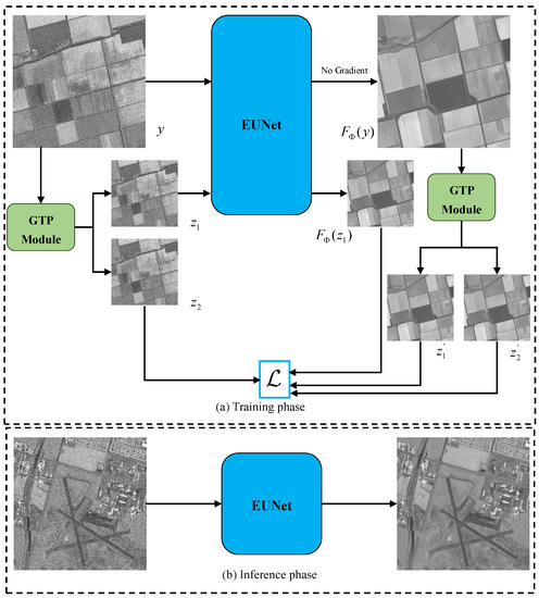
Figure 1.
Overview of the proposed SSEUNet framework. (a) Complete view of the training phase. (b) Inference phase using the trained EUNet.
3.2. Proposed GTP Module
Benefiting from noise2noise despeckling methods, we have conducted further research on the construction of noisy-noisy image pairs. According to Goodman’s theory, the fully developed speckle noise in SAR images is completely random and independently distributed noise. Therefore, we attempt to generate noisy-noisy image pairs from the real-world SAR images , where N is the total number of real-world SAR images.
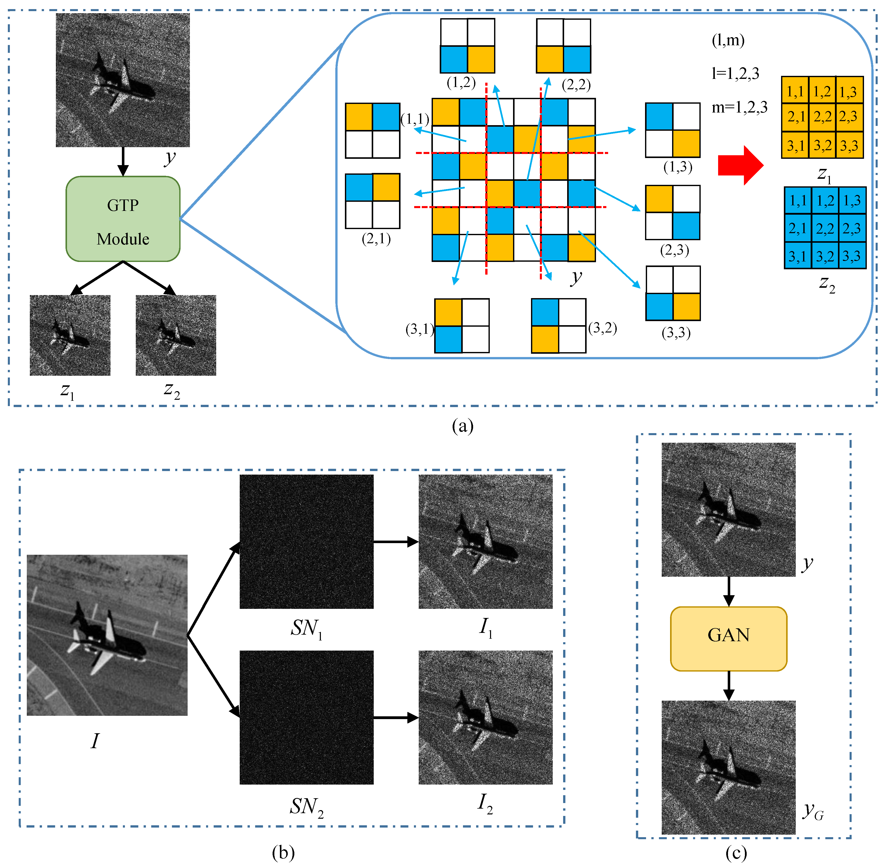
The height and width of y are H and W, respectively. The noisy-noisy image pair is the . The generation process of the proposed GTP module is divided into three steps. Firstly, the y is divided into patches, where the is a floor operation and k is the patch size. Secondly, we select a patch at the position , the two pixels of the patch are randomly extracted. The extracted pixels are used as the pixel of and at the position , respectively. Finally, for patches, the noisy-noisy image pair is obtained by repeating the second step. The size of and is . Compared with the methods of using natural images and GAN, the GTP module can directly generate noisy-noisy image pairs from real-world noisy images. Figure 2 shows three noisy-noisy image pairs generation methods, where y is the noisy image, and I is the clean natural image. and are two independent simulated speckle noise. and are simulated SAR images. is the speckled SAR image generated by GAN [35].
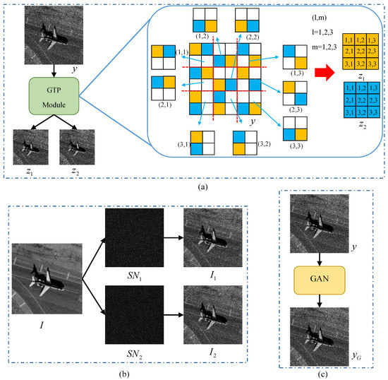
Figure 2.
Comparison of different methods for generating noisy-noisy image pairs. (a) The method of proposed GTP module. (b) The method of using natural images. (c) The method of using GAN.
In order to better explain the difference between the three generation methods, k is set to 2. When using GTP module, the y is divided into patches and the size of and is a quarter of y. In Figure 2a, the example of generating an image pair is listed right. The original image size is 6×6. The original image is divided into 9 () patches. Two pixels are randomly chosen and fill them with orange and blue respectively. The pixel filled with orange is taken as a pixel of a noisy image and the other pixel filled with blue is taken as a pixel of another noisy image . The noisy-noisy image pair is displayed as the orange image and the blue image on the right. In Figure 2b, the clean image I is element-wise multiplied with and to obtain the noisy-noisy image pair . The image size of and is . In Figure 2c, the image is obtained by using GAN. y and are combined together to construct noisy-noisy image pair . The size of y and is . By comparing the three generation methods, it can be seen that the proposed GTP module directly generates the noisy-noisy image pairs from noisy images. Meanwhile, it will not be affected by natural images or GAN performance. The size of the noisy-noisy image pairs do not affect the despeckling performance of CNNs.
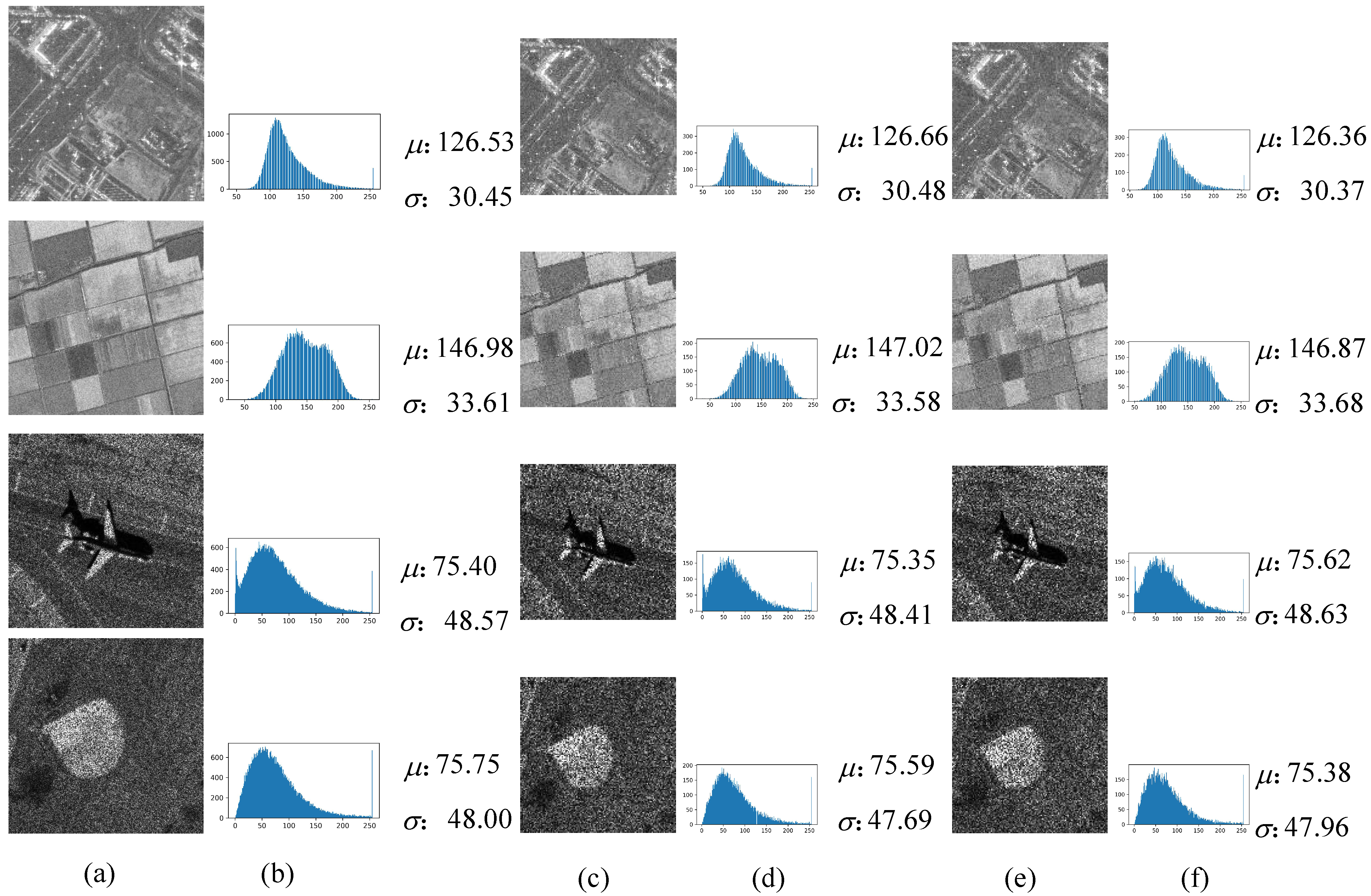
In order to verify that the noisy-noisy image pairs generated by GTP module will not change the distribution of the original noisy images, Figure 3 shows the examples of noisy-noisy image pairs generated by GTP module. In Figure 3, and are the mean and standard variance, respectively. The size of the original images is 256 × 256. The size of the noisy-noisy image pairs is 128 × 128. It can be seen that the histograms, , and visual effects are very similar.
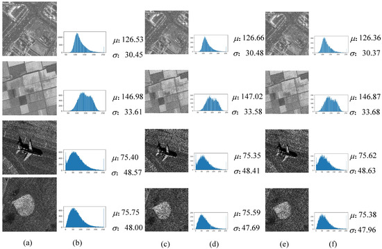
Figure 3.
Examples of noisy-noisy image pairs using GTP module. (a) Original noisy images y. (b) Histograms of y. (c) Noisy images . (d) Histograms of . (e) Noisy images . (f) Histograms of .
3.3. Enhanced U-Net
The U-Net [37] was originally proposed for medical image segmentation. It is a fully convolutional network and can be trained with very few images by using data augmentation. The U-Net is widely used in image denoising [43] and super-resolution [44]. At present, there are many variants of U-Net, which are used for various tasks. For example, the nested U-Net [45] and hybrid densely connected U-Net [46] are used for medical image segmentation. Multi-class attention-based U-Net [47] is designed for earthquake detection and seismic phase-picking.
As the speckle noise is modeled as multiplicative noise, the non-linear relationship of between noise-free SAR images and speckle noise can be obtained by a deep CNN. Therefore, an enhanced U-Net (EUNet) is designed to enhance the feature extraction and fusion capabilities of U-Net [37]. The detailed architecture of EUNet is displayed in Figure 4, where - represents the residual in residual densely connection with batch normalization (BN-RRDC) block. SSAM1-SSAM4 are sub-space attention module (SSAM) [48], respectively. ISC1-ISC4 denote the proposed improved skip connections, respectively. The and s mean the convolutional layer and stride, respectively. The and - represent concat layer and transpose convolution layers, respectively. Compared with U-Net [37], EUnet mainly has four enhancements. Firstly, we replace the convolutional layer with the BN-RRDC blocks. The BN-RRDC block is composed of residual in residual densely connections [49] and batch normalization layer, which can significantly improve the feature extraction and representation capabilities of U-Net. Meanwhile, because of the residual structure in the BN-RRDC block, the training difficulty of the EUNet will not increase.
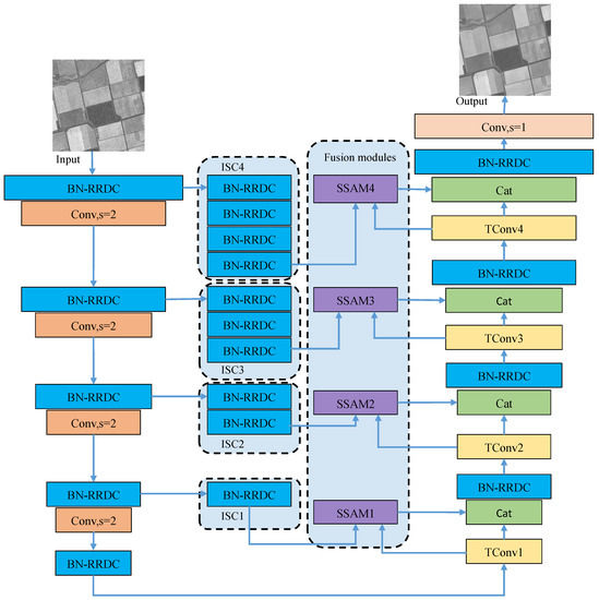
Figure 4.
The detailed architecture of EUNet.
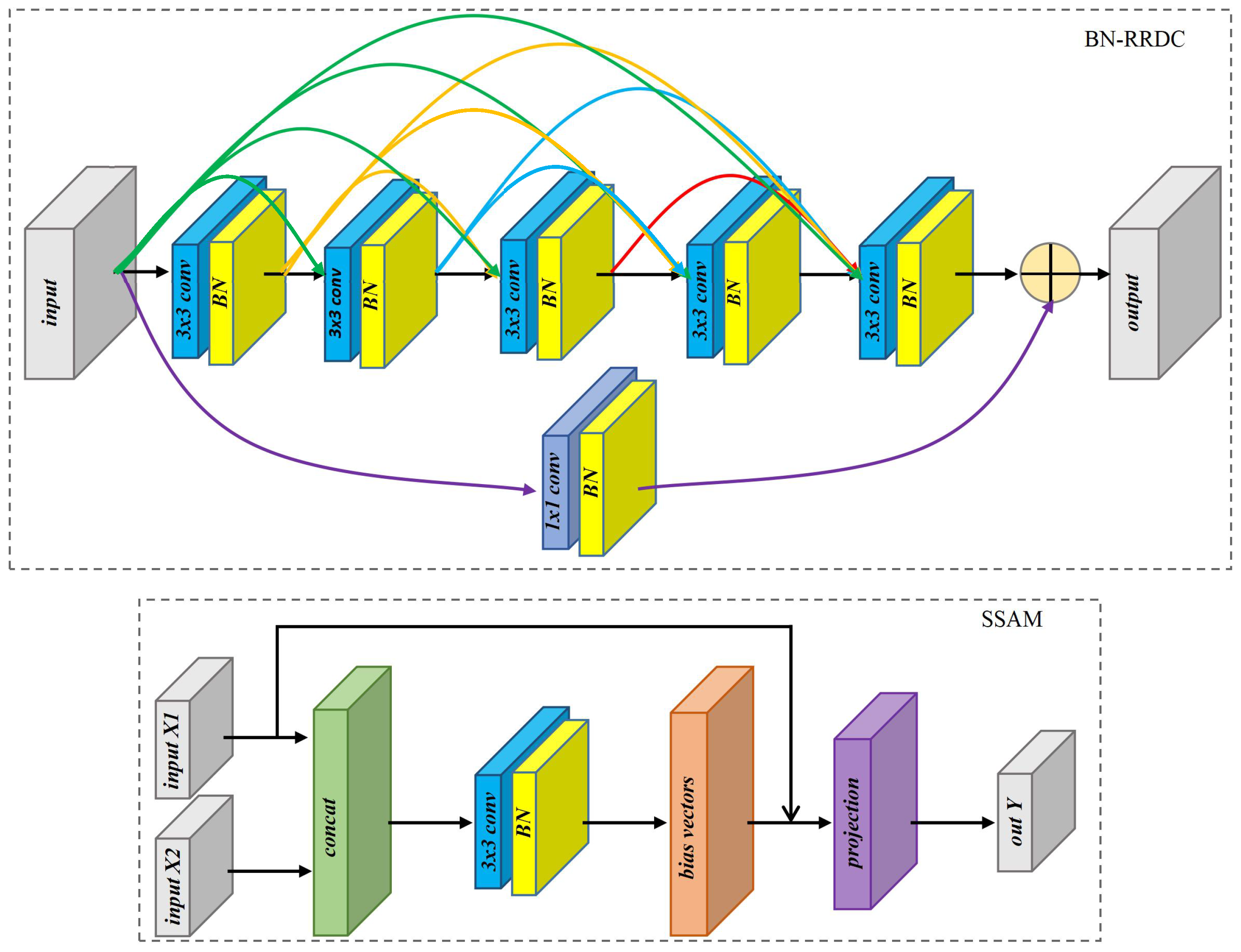
Secondly, for reducing features loss, the pooling layers are replaced by convolutional layers with . Thirdly, we design improved skip connections (ISC1-ISC4) to narrow the gap between encoder features and decoder features. In the architecture of U-Net [37], the skip connections directly send the encoder features to the decoder. In the framework of EUNet, the improved skip connections have different numbers of BN-RRDC blocks. In the structures of ISC1-ISC4, the numbers of BN-RRDC blocks are 1, 2, 3 and 4, respectively. Finally, SSAM is introduced into the feature fusion to restore weak texture and high-frequency information of the image. SSAM is a non-local sub-space attention module, which uses the non-local information to generate basis vectors through projection. The reconstructed SAR image can retain most of the original information and suppress speckle noise which is irrelevant to the basis vectors. The SSAM has been achieved state-of-the-art denoise performance for removing noise in the natural images. The detailed structure of BN-RRDC block and SSAM are displayed in Figure 5, where is the batch-normalization layer.

Figure 5.
The detailed structure of BN-RRDC block and SSAM.
3.4. Loss Function of SSEUNet
The self-supervised training method is the noise2noise method [34], which does not require clean images as targets. The noise2noise method only requires two noisy image pairs of the same image. Assuming the noisy-noisy image pair is the from the clean image x, the noise2noise tries to minimize the following loss function:
where is the denoising network and is the parameters of the denoising network. Equation (1) is the pixel-level loss function. Its optimization is the same as the supervised learning CNNs. In previous noise2noise despeckling methods, Equation (1) is commonly used loss function. Assume that the noisy SAR image is y, and the generation masks of GTP module are and . The noisy-noisy image pair is . and can be written as:
where ⊙ is the operation of GTP module. When training EUNet, Equation (1) is rewritten as:
The despeckled image pair of can be obtained by Equation (4).
where . Thus, the regularization loss can be defined as:
Meanwhile, and also can be obtained by the despeckling network , which can be written as:
In an ideal state, and are exactly the same. is the optimal despeckling network. Meanwhile, and are also exactly the same. Therefore, should be equal to 0. Equation (5) provides a regularization loss that is satisfied when a despeckling network is the optimal network . The regularization loss can narrow the gap of target pixel values between neighbors on the original noisy image. In order to exploit the regularization loss, we do not directly optimize Equation (3), but add Equation (5) to the Equation (3). Finally, the loss function of SSEUNet is defined as:
where is the hyper-parameter.
4. Experiments and Analysis
We evaluate the effectiveness of the proposed SSEUNet on simulated and real-world SAR datasets. Firstly, we report the implementation details. Secondly, the training and inference datasets, a simulated SAR dataset and a real-world SAR dataset, are introduced in detail. Thirdly, according to the fact of simulated and real-world SAR images, different evaluation metrics are selected. Finally, we present the experimental results and analysis of the simulated and real-world SAR datasets.
4.1. Implementation Details
The proposed SSEUNet does not require a pre-trained model, and it can be trained end-to-end from scratch. In the training phase, the initialization method of the network parameters is He [50]. The optimizer is Adam algorithm [51] and its momentum terms are and . The initial learning rate of SSEUNet is set to 0.00001 for the real-world experiments and 0.0001 for the simulated experiments. The learning rate reduces by reduce-on-plateau strategy and the decay ratio is 0.5. 64 × 64-sized images are used and 10 instances stack a mini-batch. The training epoch is set to 100. The hyper-parameter of in the loss function can control the strength of the regularization term. Empirically, the is set to 2 in the simulated SAR experiments and the is set to 1 in the real-world SAR experiments. In the inference phase, the input size of the trained ENUet is 256 × 256. All experiments are conducted on a workstation with Ubuntu 18.04. The hardware is an Intel Xeon(R) CPU E5-2620v3, a NVIDIA Quadro M6000 24GB GPU and 48 GB of RAM. The deep learning framework is PyTorch 1.4.0.
4.2. Datasets
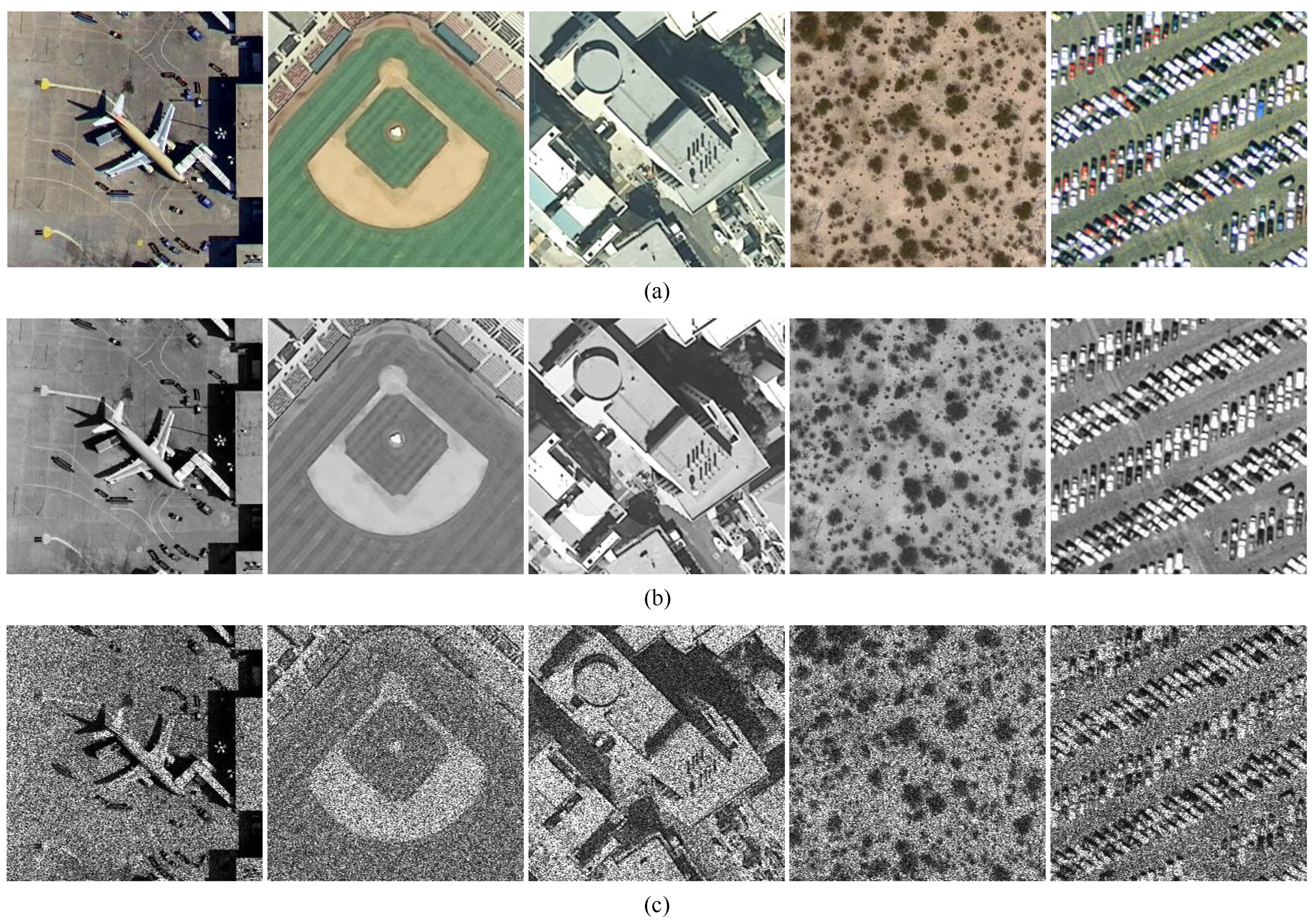
We use UC Merced Land-use (UCML) dataset [52] as a simulated dataset and it is widely used for land-use classification. The UCML dataset is a optical remote sensing dataset. The UCML dataset contains 2100 images, which are extracted from United States Geological Survey (USGS) National Map of the US regions. The resolution is 0.3 m and the size of each image is 256 × 256 × 3. To generate the simulated SAR images, we convert each image to grayscale image. Then, similar with [53], we generate simulated SAR images by multiplying simulated speckle noise to clean grayscale images. The simulated speckle noise follows Gamma distribution. In our experiments, we only considered single-look SAR images. Because of the high intensity of speckle noise in single-look SAR images, processing single-look SAR images is a very challenging case. The mean and variance of simulated speckle noise are 1. We randomly divide 2100 images into training set (1470), validation set (210) and testing set (420). In the training phase, data augmentation is used to train SSEUNet. The method of data augmentation is cropping and the crop size is 64 × 64. Finally, the augmented training set contains 213,175 patches. The size of training image pairs generated by GTP module is 32 × 32. The validation set and testing set do not use data augmentation. In Figure 6, we displays the examples of the generated simulated SAR images.
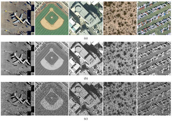
Figure 6.
Examples of simulated SAR images. (a) RGB images. (b) Grayscale images. (c) Simulated SAR images.
In order to validate the practicability of SSEUNet, seven large-scale single-look SAR images are used. They were acquired by the ICEYE SAR sensors [54]. The details of each SAR image are listed in Table 1, where the Pol., Level, Mode, Angle and Loc. are polarization type, image format, imaging mode, look angle and imaging area, respectively. The SLC, VV, SL, SM, Asc. and Des. represent the single look complex image, vertical vertical polarization, spotlight, stripmap, ascending orbit and descending orbit, respectively. We convert SLC SAR data () into amplitude SAR images (y). The generation method are as follows. Firstly, the amplitude SAR data () of SLC SAR data is obtained through Equation (8).
where and are the real data and imaginary data of , respectively. Secondly, the obtained amplitude SAR data () is normalized. The normalized method is defined as:
where means the maximum function. Finally, the normalized SAR data () is encoded for obtaining an amplitude SAR image (y). The encoding method is defined as:
where represents the minimum function and B is the encoded bit. In our experiments, B is set to 8.

Table 1.
Acquisition parameters for the ICEYE-SAR sensors.
Each amplitude SAR image (y) is cropped to 256 × 256 with a stride equal to 64. The total number of cropped images is 19,440. They are randomly divided into training set (12,800), validation set (1520) and testing set (5120). The training set uses the same data augmentation as the simulated image. The final training data has 473,600 patches. The examples of testing images are displayed in Figure 7, where the white boxes are selected regions, which are used to compute the no-reference evaluation metrics. R1–R4 are the homogeneous regions. R5–R8 are the heterogeneous regions. R9 and R10 are the whole images. These regions are excluded from training set.
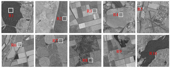
Figure 7.
Real-world SAR images for evaluating.
4.3. Evaluation Metrics
For the simulated SAR experiments, the classic evaluation metrics, peak signal-to-noise ratio (PSNR, as high as possible) [55] and structural similarity index (SSIM, as closer to 1 as possible) [56], are used. The PSNR and SSIM are defined as follows:
where the p and g are the despeckled image and the clean reference image, respectively. is the maximum signal power, i.e., 255 for grayscale images. is computed between the clean reference image and its despeckled image. The , , and represent the mean and standard variance of p and g. The is the co-variance between p and g. The and are constants.
For the real-world SAR experiments, the equivalent number of looks (ENL, as high as possible) [57], and the edge-preservation degree based on ratio of average (ER, as closer to 1 as possible) [58] are used. The ENL and ER are defined as:
where the and are the mean and standard variance of despeckled image. The i is the index set of the SAR image. The m is the total pixels of the SAR image. The asn represent the adjacent pixel values in the horizontal or vertical directions of the despeckled image, respectively. The and are the adjacent pixel values in the horizontal or vertical directions of the noisy image, respectively.
4.4. Results and Discussion
In order to demonstrate the effectiveness of SSEUNet, we compare it qualitatively and quantitatively with Lee [14], Frost [15], SAR-BM3D [18], PPB [17], MuLoG [59], SAR-CNN [22], SAR-DRN [24] and SSUNet. Lee and Frost are the local window filters. The windows are set to 5 × 5. SAR-BM3D, PPB and MuLoG belong to the class of NLM methods. The publicly available Matlab codes of SAR-BM3D, PPB and MuLoG are used and the parameters are set as suggested in the original papers. SAR-CNN and SAR-DRN are machine learning methods. We implement and train SAR-CNN and SAR-DRN from scratch on noisy-noisy dataset, following the specifics given by the authors in the original papers. The noisy-noisy dataset is generated by using natural images. Therefore, SAR-CNN and SAR-DRN are unsupervised (noise2noise) methods. SSUNet is a self-unsupervised method and the training dataa is generated by GTP module. The network of SSUNet is the U-Net [37].
4.4.1. Experiments on Simulated SAR Images
For the simulated SAR image despeckling experiments, a combination of quantitative and visual comparisons is used to analyze the effects of the different methods.
In Table 2, we show the average quantitative evaluation results obtained on simulated single-look SAR images with the best performance marked in bold and the second-best marked in underlined. and are the inference average speed and the number of parameters, respectively. represents gigabit floating-point operations per second. and are not marked the best and the second-best. The reason is that the values of and can not reflect the performance of despeckling methods. The results are computed as the average over the 420 testing images. The local window methods and NLM methods are grounded on the middle part of the table, while noise2noise methods are listed in the lower part. The difference between SSUNet and SSEUNet is the network. The network of SSUNet is the U-Net [37]. The network of SSEUNet is the proposed EUNet. The results of SSUNet and SSEUNet are to verify that EUNet has better despeckling performance than U-Net.
Table 2.
Numerical results on simulated single-look images.
As can be seen from Table 2, the proposed SSEUNet outperform other methods on the MSE, PSNR and SSIM. Looking at the PSNR and SSIM metrics, noise2noise methods appear to have the potential to provide a clear performance gain over conventional ones. Indeed, although the performance of SAR-CNN is similar to that of the advanced NLM method, SSEUNet is about 1 dB and 0.0536 higher than the best method (SAR-BM3D). But the time it takes to process a image with 256 × 256 is approximately 157 times faster. By comparing the results of SAR-CNN and SAR-DRN, the more layers of the network, the better the despeckling performance. However, the network with dilated convolution layer (SAR-DRN) can improve the details of the despeckled image. In addition, compared with the second-best results (SSUNet), the proposed SSEUNet achieved a 0.5 dB and 0.0323 improvement, respectively. From the results of SSEUNet and SSUNet, we can find that our improvement to U-Net is effective and the increase of parameters does not significantly reduce the inference speed.
Visual evaluation is another way to qualitatively evaluate the despeckling performance of different methods. To visualize the despeckling results of proposed SSEUNet and other methods, Figure 8 shows the despeckled visual results of a simulated SAR image. The is the result of using SSEUNet. It can be seen from the visual results that all despeckling methods can remove speckle noise to a certain extent. But the best despeckling results is achieved by the based on noise2noise methods. The results of the local window methods are too smooth, which causes the image to be blurred, so that the despeckled images lose the boundary information of the image. Compared with the local window methods, the effect of the NLM methods is significantly improved. However, looking at the results of PPB, there is a ringing effect at the boundary, which distorts the image boundary. In the noise2noise methods, as the network depth deepens, the better the despeckling effect, the clearer the image. It can be seen that proposed SSEUNet () shows the best ability to reduce speckle noise and retain texture structure.
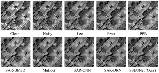
Figure 8.
Visual results of simulated images.
4.4.2. Experiments on Real-World SAR Images
In order to further illustrate the practicability of the proposed method, the real-world SAR images are used for the experiments. The real-world SAR images are detailed introduced in Section 4.2. Table 3 lists the quantitative evaluation results of ENL over the selected regions. These selected regions are shown in Figure 7, where R1–R4 are homogeneous regions.
Table 3.
ENL results on real-world SAR images.
Clearly, as listed by the ENL values in Table 3, the noise2noise methods show better despeckling performance in homogeneous regions. In the local window methods, the Lee and Frost algorithms show similar despeckling performance. In the NLM methods, the PPB algorithm has the worst despeckling ability. The despeckling ability of SAR-BM3D and MuLoG is similar. Although SAR-DRN and SA-CNN show subtle advantages over NLM methods, the proposed SSEUNet has improved 20.31, 6.46, 24.95 and 509.02 in the four regions over the MuLoG method, respectively. Since the SAR-DRN and SAR-CNN methods use training image pairs generated from natural images, they cannot learn the relationship between speckle noise and noise-free SAR images. Compared with SAR-CNN and SAR-DRN, the despeckling performance of SSUNet is significantly improved. The results SSUNet is obtained through using GTP module to generate noisy-noisy image pairs. In addition, comparing the results of SSUNet and SSEUNet, the EUNet has a stronger despeckling ability than U-Net. In general, the proposed SSEUNet can better process real-world SAR images.
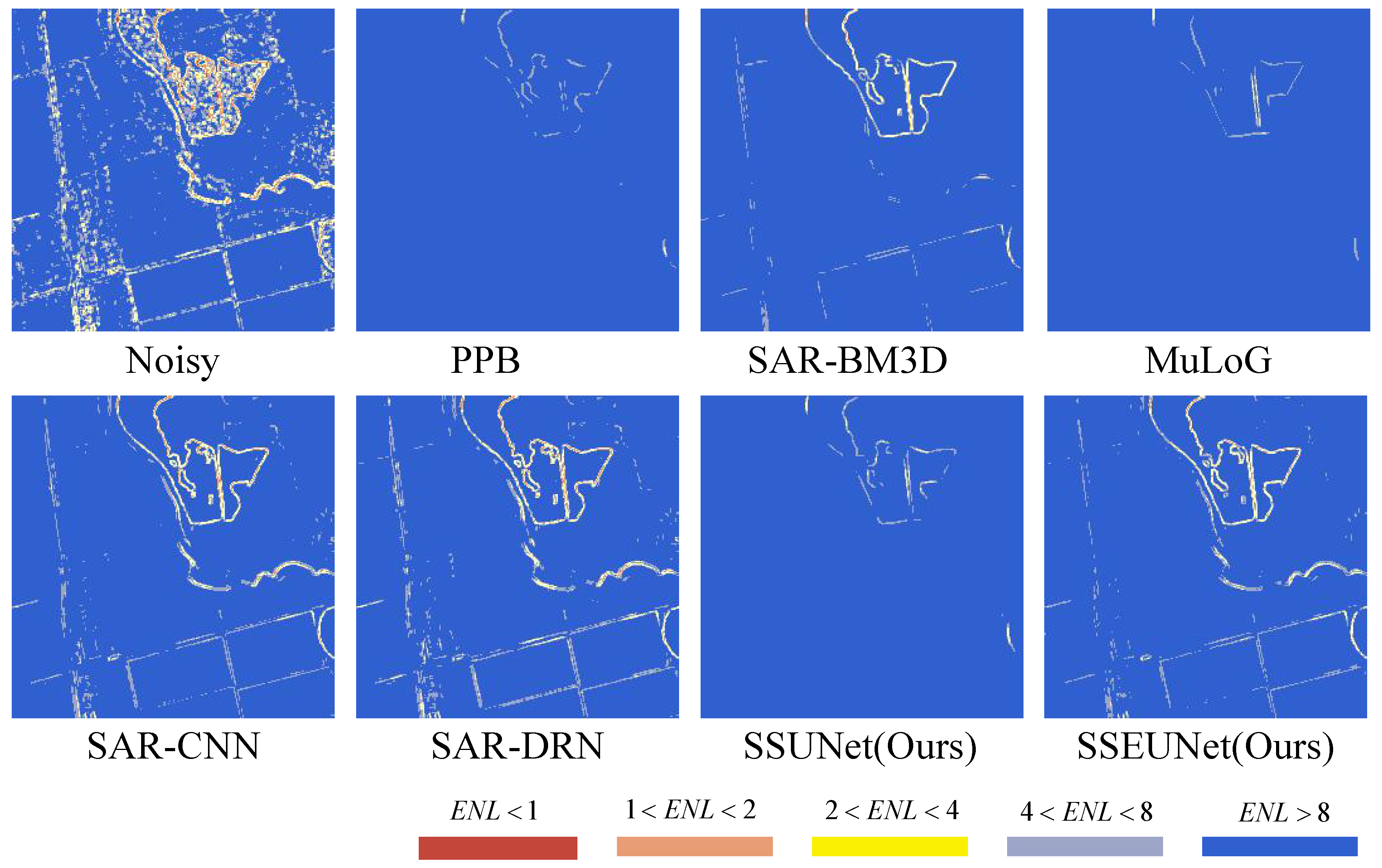
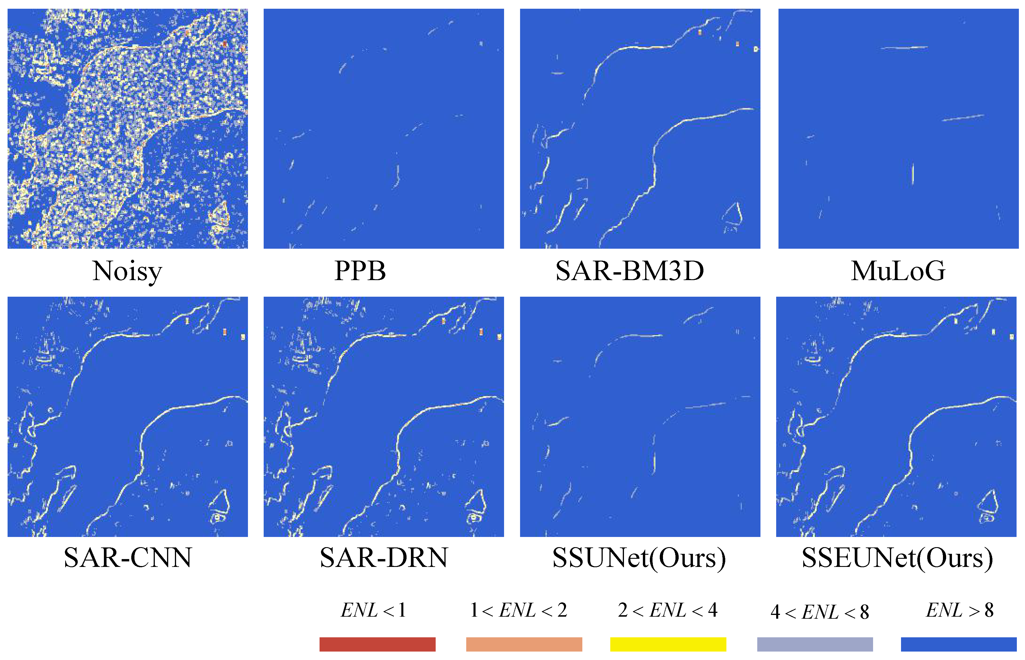
Generally, ENL can reflect the effectiveness of the algorithm, to some extent, but perfectly homogeneous regions are rare in the real-world SAR images. Therefore, an no-reference estimated approach, which is called the , is used to demonstrate the effectiveness of the proposed SSEUNet. The involves calculating small ENLs by using a sliding window (set to 3 × 3) until the whole SAR image is covered [60]. Figure 9 and Figure 10 show the ENL maps of R9 and R10, which are listed in Figure 7. We only show the ENL maps of the NLM and noise2noise despeckling methods. The reason is that the results of local window methods are too smooth, resulting in a very average ENL value of the despeckled images. The ENL value should have a small change in the heterogeneous region, or even zero. However, it should have a greater improvement in the homogeneous region. This point is proven and shown in Figure 9 and Figure 10. The ENL maps also show that the ability of details losses. From the ENL maps, the most details losses are PPB and MuLoG. Compared with SAR-BM3D, the noise2noise methods can not only better protect the image details, but also better remove the speckle noise. In the noise2noise methods, the proposed SSEUNet has the best despeckling and detail protection ability.
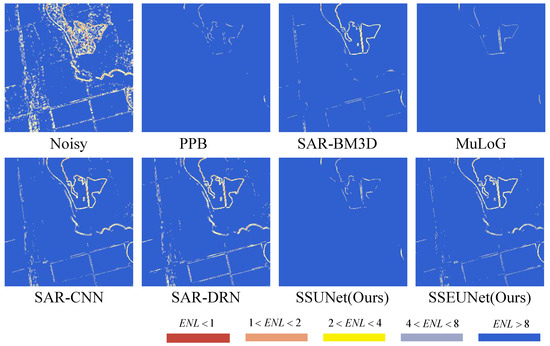
Figure 9.
ENL maps of different despeckling methods on R9.
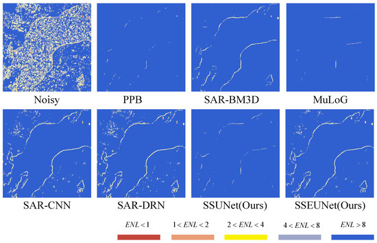
Figure 10.
ENL maps of different despeckling methods on R10.
Table 4 displays the numerical results of ER metric on the R5–R8 regions, where V and H are the vertical and horizontal results of the ER metric. It can be seen that the proposed SSEUNet have obvious advantages in protecting horizontal and vertical structures. In the noise2noise methods, the proposed GTP module and EUNet can better process real-word SAR images. The proposed GTP module can use real-world SAR images to construct noisy-noisy image pairs to train deep CNNs, so that the network can better learn the relationship of speckle noise and noise-free SAR images.
Table 4.
ER metric on real-world SAR images.
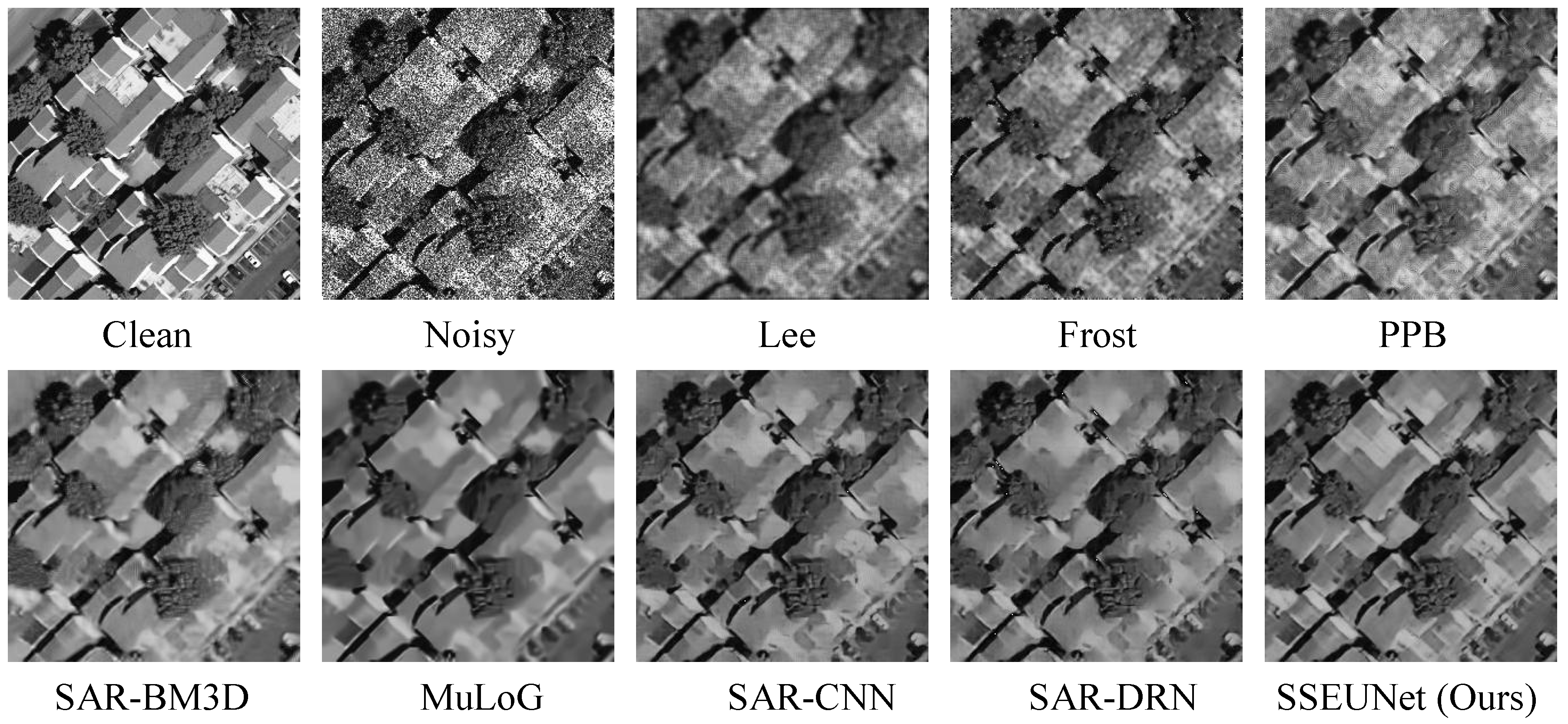
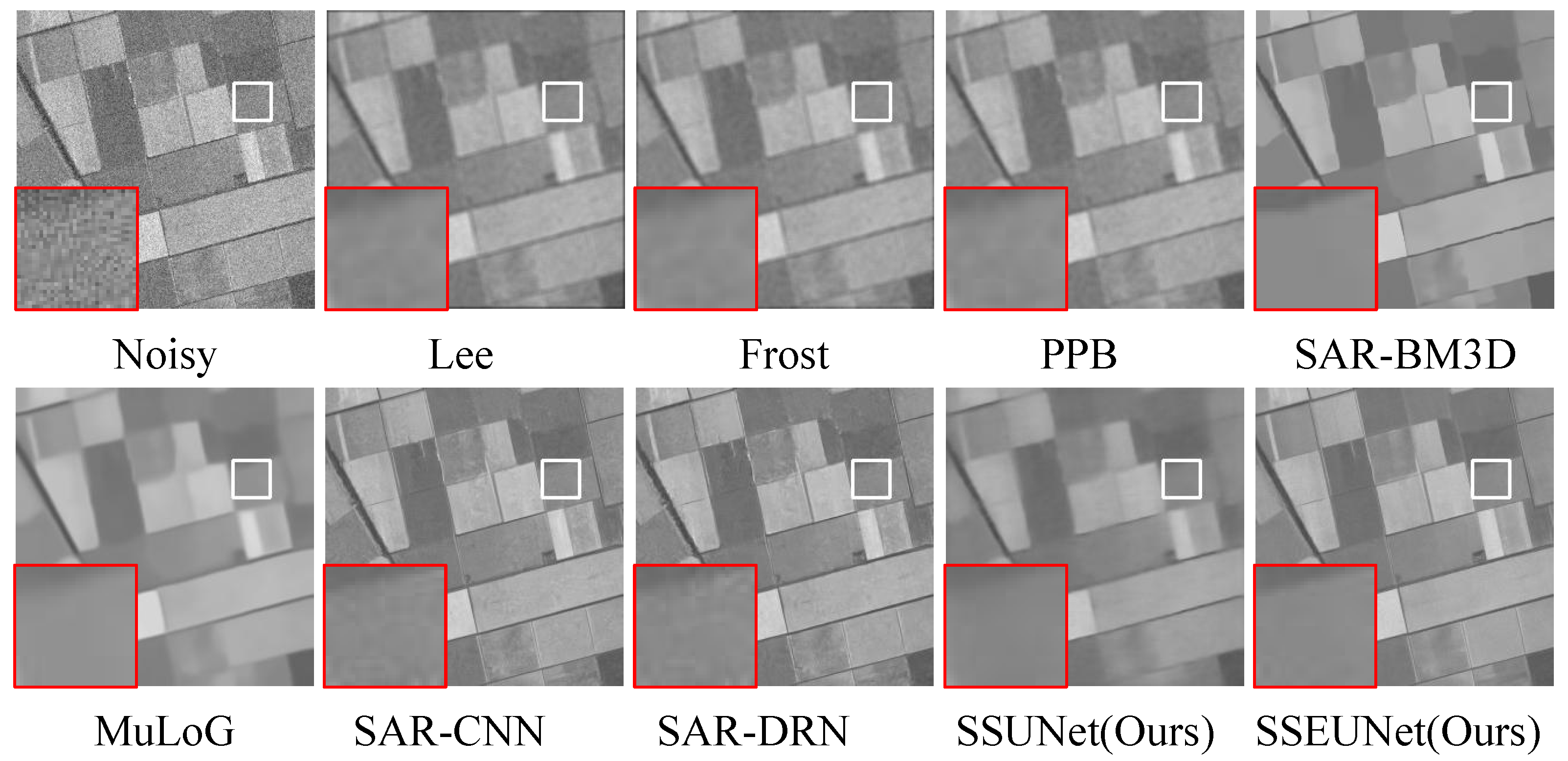
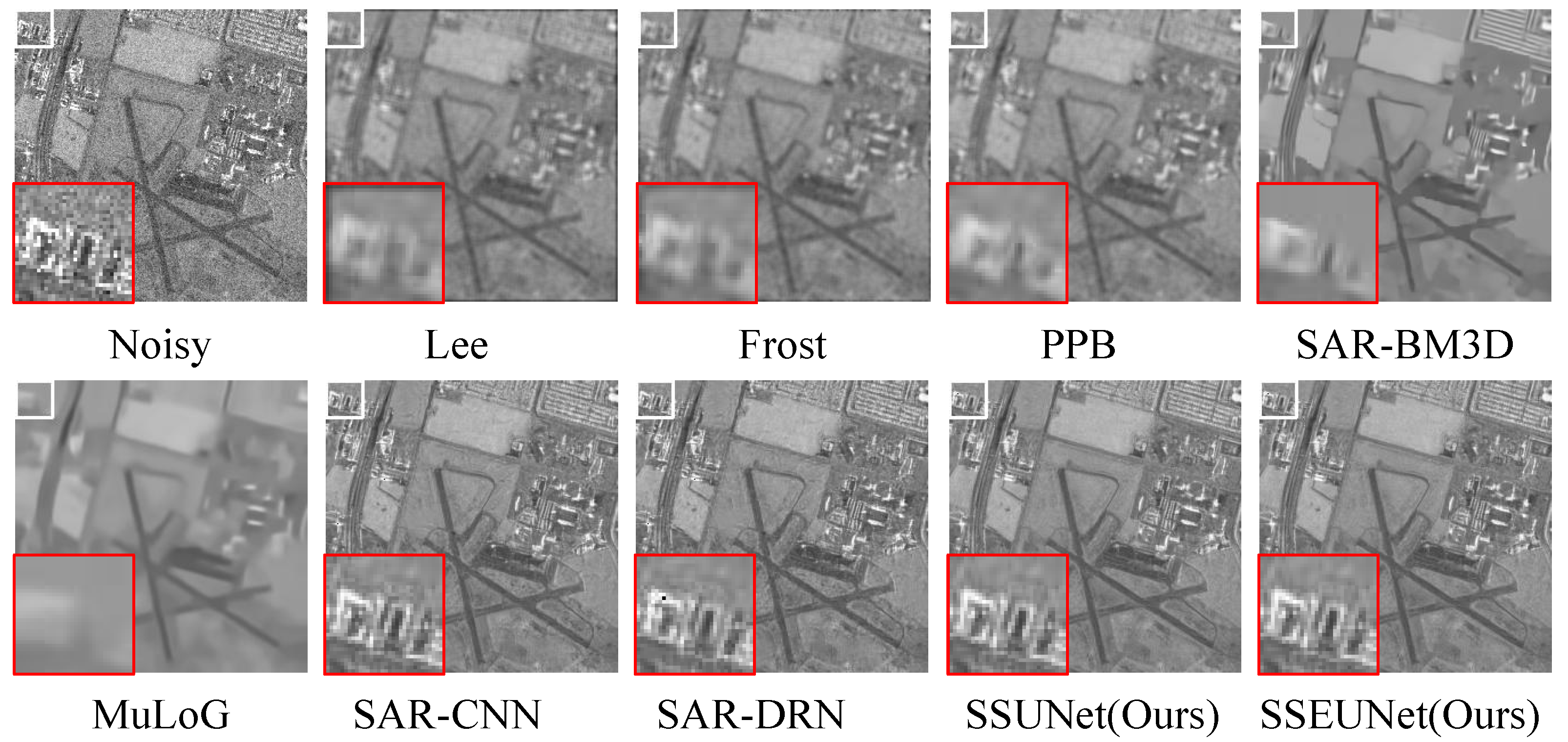
It is worth carefully studying different methods of despeckled SAR images. Figure 11 and Figure 12 shows the details of homogeneous and heterogeneous regions in the real-world SAR images, respectively. It can be seen from the results that the local window methods are too smooth to lose the contrast. Loss the contrast means that the despeckled images structure using local window filters becomes smooth, and the structural contrast between edges and non-edges becomes blurred. In addition, many strong points and linear structures are lost in the NLM despeckling methods. The result of PPB can also cause a ringing effect at the boundary. Compared with other traditional methods, the result of SAR-BM3D performs best and provides an acceptable balance between smoothing and details preservation. Among SAR-DRN, SAR-CNN and SSEUNet methods, the result of SSEUNet is the best. Figure 13 shows the visualization despeckling results of different scenes. It can be seen from the despeckled results that the proposed SSEUNet can deal with real-world SAR images in different scenes.
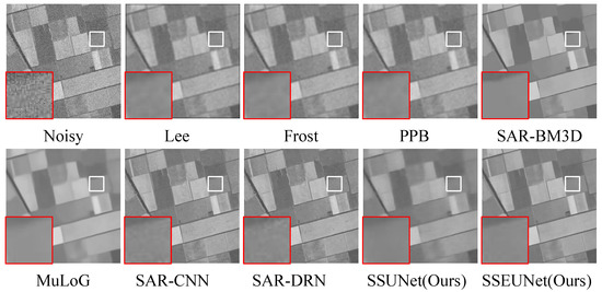
Figure 11.
Visual results of homogeneous regions on real-word SAR images.
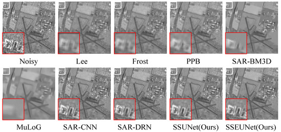
Figure 12.
Visual results of heterogeneous regions on real-word SAR images.
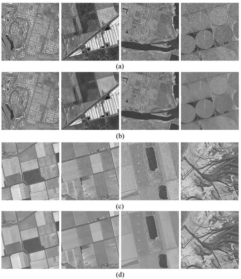
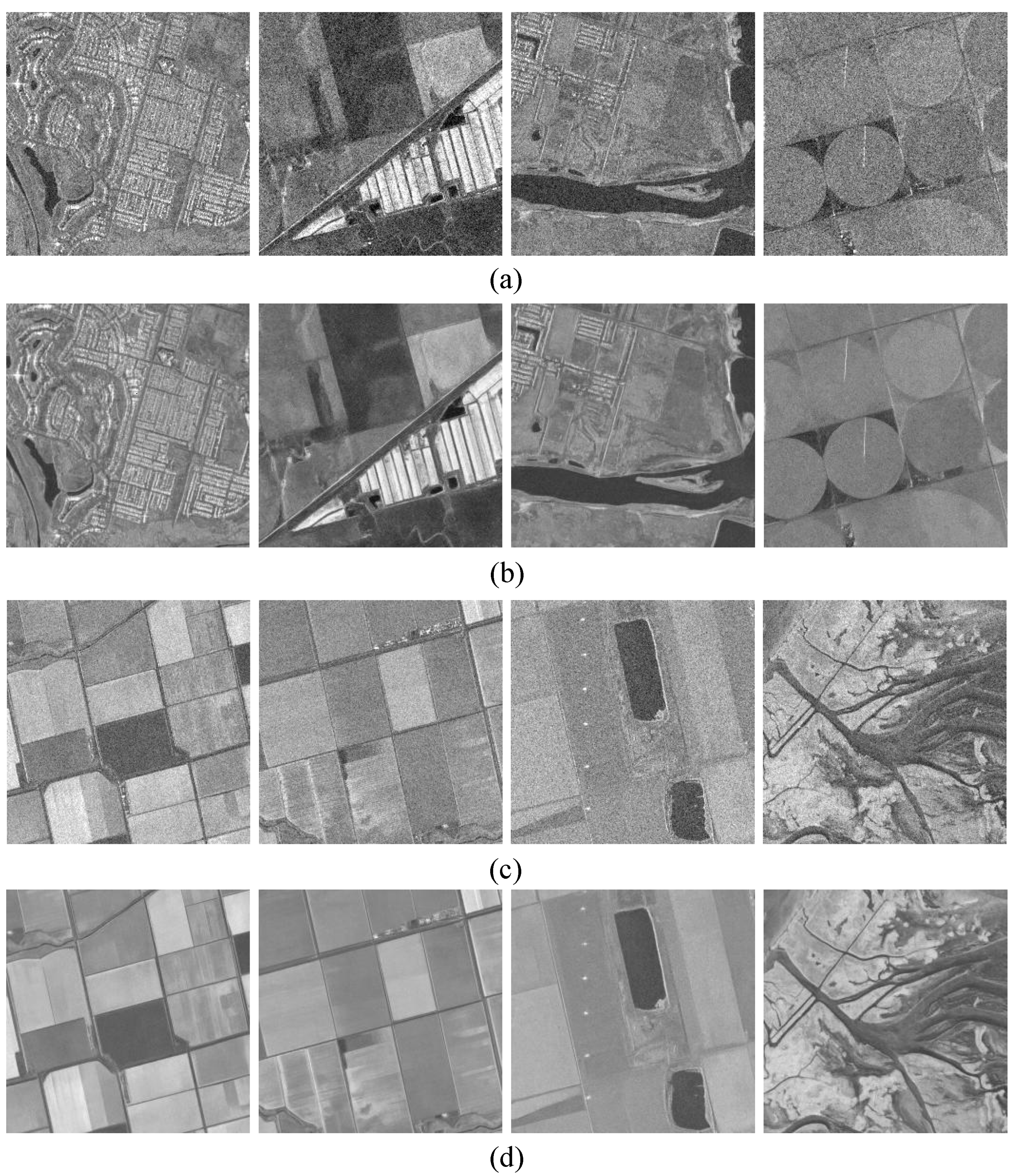
Figure 13.
The despeckled results of the SSEUNet in real-world SAR images. (a,c) Real-world SAR images. (b,d) Despeckled results.
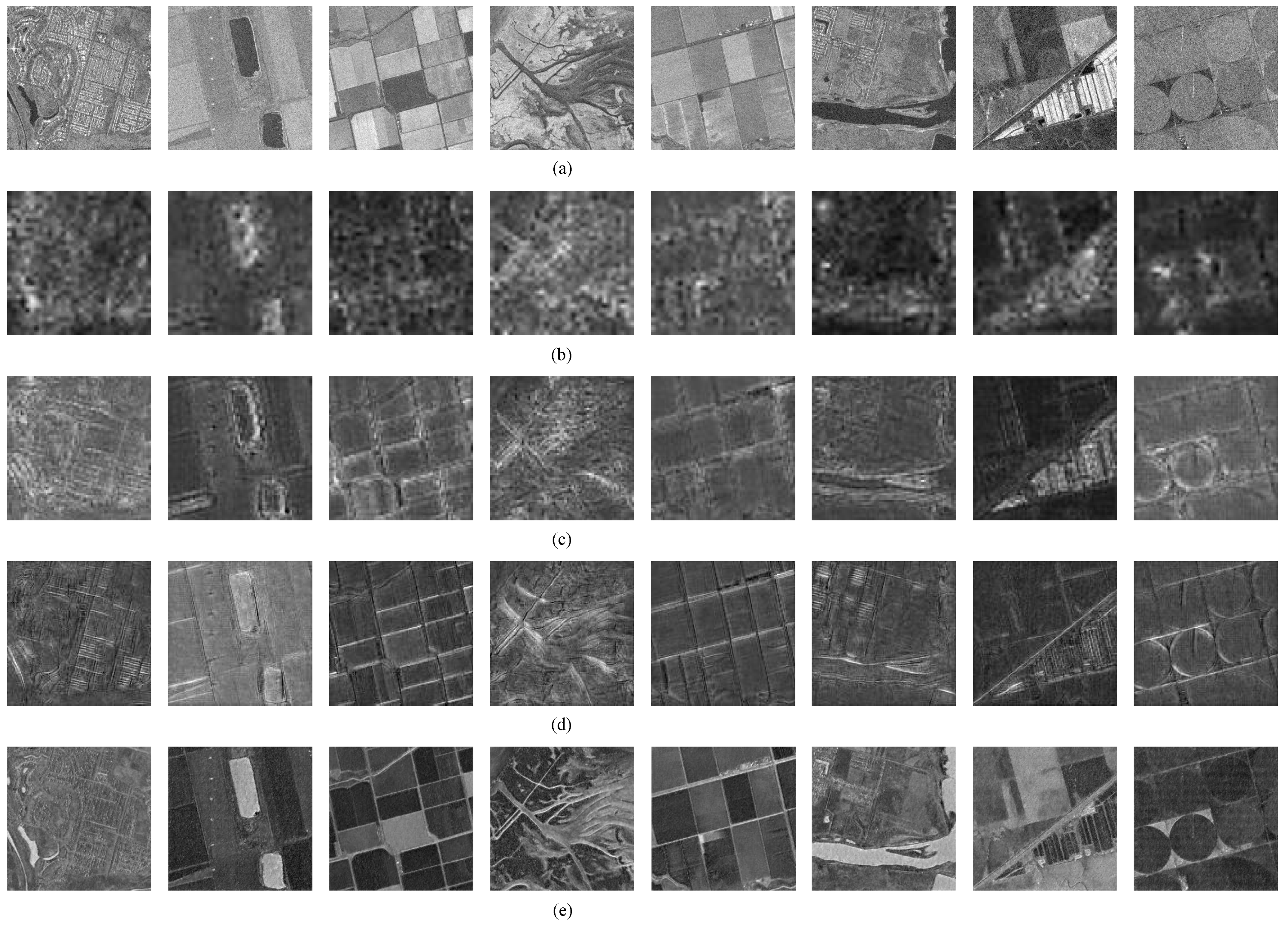
To gain insight about how the learned SSAM on the real-world SAR images, we pick 8 sample images and inspect the output features of SSAM. As can be seen from Figure 4, the input features of SSAM1 are the output features of ISC1 and TConv1. The inputs of SSAM2 are the outputs of ISC2 and TConv2. The outputs of ISC3 and TConv3 are fed into SSAM3. The input features of SSAM4 are the outputs of ISC4 and TConv4. The output features of SSAM1-SSAM4 are extracted from the layer in the SSAM1-SSAM4. The structure of SSAM1-SSAM4 are exactly the same. The detailed structure of SSAM is shown in Figure 5. The output feature sizes of SSAM1-SSAM4 are 256 × 32 × 32, 128 × 64 × 64, 64 × 128 × 128 and 32 × 256 × 256, respectively. In the process of visualization, we perform averaging operations on the output features of SSAM1-SSAM4. Each visualization feature is the mean features of all channels. The sizes of visualization features are 32 × 32, 64 × 64, 128 × 128 and 256 × 256 in the SSAM1-SSAM4, respectively. Figure 14 shows the visualization features of SSAM1-SSAM4. It can be seen that the details of weak texture and structure are gradually restored from noisy SAR images.
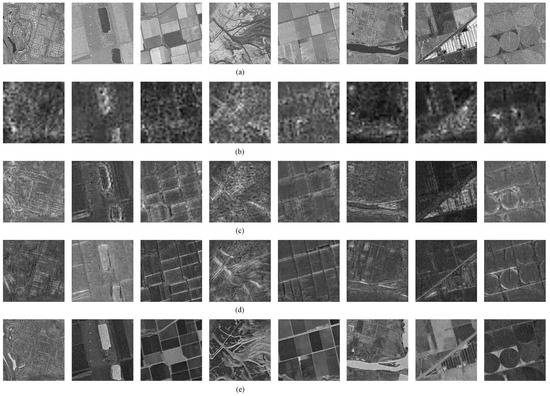
Figure 14.
Visualization features of SSAM1-SSAM4. (a) Original SAR images. (b–e) The visualization features of SSAM1-SSAM4.
5. Conclusions
In this paper, we propose a novel self-supervised despeckling algorithm with an enhanced U-Net (SSEUNet). The proposed SSEUNet is composed of generation training pairs (GTP) module, enhanced U-Net (EUNet) and a self-supervised training loss function with a regularization loss. The proposed SSEUNet has the following advantages. Firstly, unlike previous self-supervised despeckling works, the noisy-noisy image pairs are generated from real-word SAR images through a novel generation training pairs module, which makes it possible to train deep convolutional neural networks using real-world SAR images. The GTP module can eliminate the effects of natural images, time series images and the performance of GAN. Secondly, the EUNet is designed to improve the features extraction and fusion capabilities of the U-Net. Compared with U-Net, we introduce BN-RRDC blocks, convolutional layers with , improved skip connections and SSAM. Although the EUNet has more parameters and more complex structure, the training difficulty will not increase. The reason is that there is the residual structures in the BN-RRDC block. Thirdly, a self-supervised training loss function is designed to address the difference of target pixel values between neighbors on the original noisy image. The loss function includes a reconstruction loss (MSE) and a regularization loss. Finally, visual and quantitative experiments on simulated and real-world SAR images show that the proposed SSEUNet notably reduces speckle noise with better preserving features, which exceed several state-of-the-art despeckling methods.
However, the inference speed of proposed SSEUNet needs to be improved. The proposed SSEUNet uses complex feature extraction block and sub-space attention modules, which leads to a longer time for evaluating an image. At the same time, the despeckling results of different data augmentation methods also need to be verified on the SAR images. In the future, we plan to explore two works. Firstly, we will explore a lightweight network to replace EUNet for improving inference speed. Secondly, the despeckling effects of different data augmentation methods will be verified.
Author Contributions
Conceptualization, G.Z.; Data curation, G.Z. and S.L.; Formal analysis, G.Z.; Investigation, G.Z. and X.L.; Methodology, G.Z. and X.L.; Resources, Z.L.; Software, G.Z.; Supervision, Z.L.; Validation, G.Z. and X.L.; Visualization, G.Z.; Writing—original draft, G.Z. and X.L. All authors have read and agreed to the published version of the manuscript.
Funding
This research was supported by the National Science Foundation for Distinguished Young Scholars, Grant Numbers 61906213.
Institutional Review Board Statement
Not applicable.
Informed Consent Statement
Not applicable.
Data Availability Statement
UC Merced land-use dataset is available are http://vision.ucmerced.edu/datasets, accessed on 27 October 2021. ICEYE SAR dataset is available at https://www.iceye.com/sar-data, accessed on 27 October 2021.
Conflicts of Interest
The authors declare no conflict of interest.
References
- Moreira, A.; Prats-Iraola, P.; Younis, M.; Krieger, G.; Hajnsek, I.; Papathanassiou, K.P. A tutorial on synthetic aperture radar. IEEE Geosci. Remote Sens. Mag. 2013, 1, 6–43. [Google Scholar] [CrossRef] [Green Version]
- Yang, Z.; Wei, J.; Deng, J.; Gao, Y.; Zhao, S.; He, Z. Mapping Outburst Floods Using a Collaborative Learning Method Based on Temporally Dense Optical and SAR Data: A Case Study with the Baige Landslide Dam on the Jinsha River, Tibet. Remote Sens. 2021, 13, 2205. [Google Scholar] [CrossRef]
- Qin, Y.; Xiao, X.; Wang, J.; Dong, J.; Ewing, K.; Hoagland, B.; Hough, D.J.; Fagin, T.D.; Zou, Z.; Geissler, G.L.; et al. Mapping Annual Forest Cover in Sub-Humid and Semi-Arid Regions through Analysis of Landsat and PALSAR Imagery. Remote Sens. 2016, 8, 933. [Google Scholar] [CrossRef] [Green Version]
- Zhang, T.; Zhang, X.; Ke, X.; Zhan, X.; Shi, J.; Wei, S.; Pan, D.; Li, J.; Su, H.; Zhou, Y.; et al. LS-SSDD-v1.0: A Deep Learning Dataset Dedicated to Small Ship Detection from Large-Scale Sentinel-1 SAR Images. Remote Sens. 2020, 12, 2997. [Google Scholar] [CrossRef]
- Zhang, T.; Zhang, X.; Ke, X.; Liu, C.; Xu, X.; Zhan, X.; Wang, C.; Ahmad, I.; Zhou, Y.; Pan, D.; et al. HOG-ShipCLSNet: A Novel Deep Learning Network with HOG Feature Fusion for SAR Ship Classification. IEEE Trans. Geosci. Remote Sens. 2021. [Google Scholar] [CrossRef]
- Herzfeld, U.C.; Williams, S.; Heinrichs, J.; Maslanik, J.; Sucht, S. Geostatistical and Statistical Classification of Sea-Ice Properties and Provinces from SAR Data. Remote Sens. 2016, 8, 616. [Google Scholar] [CrossRef] [Green Version]
- Singh, P.; Diwakar, M.; Shankar, A.; Shree, R.; Kumar, M. A Review on SAR Image and its Despeckling. Arch. Comput. Methods Eng. 2021. [Google Scholar] [CrossRef]
- Argenti, F.; Lapini, A.; Bianchi, T.; Alparone, L. A Tutorial on Speckle Reduction in Synthetic Aperture Radar Images. IEEE Geosci. Remote Sens. Mag. 2013, 1, 6–35. [Google Scholar] [CrossRef] [Green Version]
- Zhang, T.; Zhang, X.; Shi, J.; Wei, S.; Wang, J.; Li, J.; Su, H.; Zhou, Y. Balance Scene Learning Mechanism for Offshore and Inshore Ship Detection in SAR Images. IEEE Geosci. Remote Sens. Lett. 2020, 1–5. [Google Scholar] [CrossRef]
- Zhang, T.; Zhang, X. ShipDeNet-20: An Only 20 Convolution Layers and <1-MB Lightweight SAR Ship Detector. IEEE Geosci. Remote Sens. Lett. 2021, 18, 1234–1238. [Google Scholar]
- Zhang, T.; Zhang, X. A Polarization Fusion Network with Geometric Feature Embedding for SAR Ship Classification. Pattern Recognit. 2021, 123, 108365. [Google Scholar] [CrossRef]
- Zhang, T.; Zhang, X. Squeeze-and-Excitation Laplacian Pyramid Network with Dual-Polarization Feature Fusion for Ship Classification in SAR Images. IEEE Geosci. Remote Sens. Lett. 2021, 1. [Google Scholar] [CrossRef]
- Wei, Y.; Li, Y.; Ding, Z.; Wang, Y.; Zeng, T.; Long, T. SAR Parametric Super-Resolution Image Reconstruction Methods Based on ADMM and Deep Neural Network. IEEE Trans. Geosci. Remote Sens. 2021. [Google Scholar] [CrossRef]
- Lee, J.S. Speckle analysis and smoothing of synthetic aperture radar images. Comput. Graph. Image Process. 1981, 17, 24–32. [Google Scholar] [CrossRef]
- Frost, V.S.; Stiles, J.A.; Shanmugan, K.S.; Holtzman, J.C. A Model for Radar Images and Its Application to Adaptive Digital Filtering of Multiplicative Noise. IEEE Trans. Pattern Anal. Mach. Intell. 1982, 4, 157–166. [Google Scholar] [CrossRef]
- Kuan, D.T.; Sawchuk, A.A.; Strand, T.C.; Chavel, P. Adaptive Noise Smoothing Filter for Images with Signal-Dependent Noise. IEEE Trans. Pattern Anal. Mach. Intell. 1985, 7, 165–177. [Google Scholar] [CrossRef]
- Deledalle, C.; Denis, L.; Tupin, F. Iterative Weighted Maximum Likelihood Denoising with Probabilistic Patch-Based Weights. IEEE Signal Process. 2009, 18, 2661–2672. [Google Scholar] [CrossRef] [PubMed] [Green Version]
- Parrilli, S.; Poderico, M.; Angelino, C.V.; Verdoliva, L. A Nonlocal SAR Image Denoising Algorithm Based on LLMMSE Wavelet Shrinkage. IEEE Geosci. Remote Sens. 2012, 50, 606–616. [Google Scholar] [CrossRef]
- Deledalle, C.A.; Denis, L.; Tupin, F.; Reigber, A.; Jager, M. NL-SAR: A unified nonlocal framework for resolution-preserving (Pol)(In)SAR denoising. IEEE Trans. Geosci. Remote Sens. 2015, 53, 2021–2038. [Google Scholar] [CrossRef] [Green Version]
- Zhang, T.; Zhang, X.; Li, J.; Xu, X.; Wang, B.; Zhan, X.; Xu, Y.; Ke, X.; Zeng, T.; Su, H.; et al. SAR Ship Detection Dataset (SSDD): Official Release and Comprehensive Data Analysis. Remote Sens. 2021, 13, 3690. [Google Scholar] [CrossRef]
- Zhang, T.; Zhang, X.; Shi, J.; Wei, S. HyperLi-Net: A hyper-light deep learning network for high-accurate and high-speed ship detection from synthetic aperture radar imagery. ISPRS J. Photogramm. Remote Sens. 2020, 167, 123–153. [Google Scholar] [CrossRef]
- Chierchia, G.; Cozzolino, D.; Poggi, G.; Verdoliva, L. SAR image despeckling through convolutional neural networks. In Proceedings of the IEEE International Geoscience and Remote Sensing Symposium, Fort Worth, TX, USA, 23–28 July 2017; pp. 5438–5441. [Google Scholar]
- Cozzolino, D.; Verdoliva, L.; Scarpa, G.; Poggi, G. Nonlocal CNN SAR Image Despeckling. Remote Sens. 2020, 12, 1006. [Google Scholar] [CrossRef] [Green Version]
- Zhang, Q.; Yuan, Q.; Li, J.; Zhen, Y.; Zhang, L. Learning a Dilated Residual Network for SAR Image Despeckling. Remote Sens. 2018, 10, 196. [Google Scholar] [CrossRef] [Green Version]
- Gui, Y.; Xue, L.; Li, X. SAR image despeckling using a dilated densely connected network. Remote Sens. Lett. 2018, 9, 857–866. [Google Scholar] [CrossRef]
- Shen, H.; Zhou, C.; Li, J.; Yuan, Q. SAR Image Despeckling Employing a Recursive Deep CNN Prior. IEEE Geosci. Remote Sens. 2021, 59, 273–286. [Google Scholar] [CrossRef]
- Dalsasso, E.; Denis, L.; Tupin, F. SAR2SAR: A Semi-Supervised Despeckling Algorithm for SAR Images. IEEE J. Sel. Top. Appl. Earth Obs. Remote Sens. 2021, 14, 4321–4329. [Google Scholar] [CrossRef]
- Yuan, Y.; Sun, J.; Guan, J. Blind SAR Image Despeckling Using Self-Supervised Dense Dilated Convolutional Neural Network. arXiv 2019, arXiv:1908.01608. [Google Scholar]
- Molini, A.B.; Valsesia, D.; Fracastoro, G.; Magli, E. Speckle2Void: Deep Self-Supervised SAR Despeckling with Blind-Spot Convolutional Neural Networks. IEEE Geosci. Remote Sens. 2021. [Google Scholar] [CrossRef]
- Yuan, Y.; Guan, J.; Feng, P.; Wu, Y. A Practical Solution for SAR Despeckling with Adversarial Learning Generated Speckled-to-Speckled Images. IEEE Geosci. Remote Sens. Lett. 2020. [Google Scholar] [CrossRef]
- Ma, X.; Wang, C.; Yin, Z.; Wu, P. SAR Image Despeckling by Noisy Reference-Based Deep Learning Method. IEEE Geosci. Remote Sens. 2020, 58, 8807–8818. [Google Scholar] [CrossRef]
- Pan, T.; Peng, D.; Yang, W.; Li, H.C. A Filter for SAR Image Despeckling Using Pre-Trained Convolutional Neural Network Model. Remote Sens. 2019, 11, 2379. [Google Scholar] [CrossRef] [Green Version]
- Li, J.; Li, Y.; Xiao, Y.; Bai, Y. HDRANet: Hybrid Dilated Residual Attention Network for SAR Image Despeckling. Remote Sens. 2019, 11, 2921. [Google Scholar] [CrossRef] [Green Version]
- Lehtinen, J.; Munkberg, J.; Hasselgren, J.; Laine, S.; Karras, T.; Aittala, M.; Aila, T. Noise2Noise: Learning Image Restoration without Clean Data. arXiv 2018, arXiv:1803.04189. [Google Scholar]
- Goodfellow, I.J.; Pouget-Abadie, J.; Mirza, M.; Xu, B.; Warde-Farley, D.; Ozair, S.; Courville, A.C.; Bengio, Y. Generative Adversarial Networks. arXiv 2014, arXiv:1406.2661. [Google Scholar] [CrossRef]
- Mullissa, A.G.; Marcos, D.; Tuia, D.; Herold, M.; Reiche, J. deSpeckNet: Generalizing Deep Learning-Based SAR Image Despeckling. IEEE Geosci. Remote Sens. 2020. [Google Scholar] [CrossRef]
- Ronneberger, O.; Fischer, P.; Brox, T. U-Net: Convolutional Networks for Biomedical Image Segmentation. In Proceedings of the Medical Image Computing and Computer-Assisted Intervention, Munich, Germany, 5–9 October 2015; Volume 9351. [Google Scholar]
- Zhang, K.; Zuo, W.; Chen, Y.; Meng, D.; Zhang, L. Beyond a Gaussian Denoiser: Residual Learning of Deep CNN for Image Denoising. IEEE Signal Process. 2017, 26, 3142–3155. [Google Scholar] [CrossRef] [PubMed] [Green Version]
- Zhang, J.; Li, W.; Li, Y. SAR Image Despeckling Using Multiconnection Network Incorporating Wavelet Features. IEEE Geosci. Remote Sens. Lett. 2020, 17, 1363–1367. [Google Scholar] [CrossRef]
- Vitale, S.; Ferraioli, G.; Pascazio, V. Multi-Objective CNN-Based Algorithm for SAR Despeckling. IEEE Geosci. Remote Sens. 2020. [Google Scholar] [CrossRef]
- Martino, G.D.; Poderico, M.; Poggi, G.; Riccio, D.; Verdoliva, L. Benchmarking framework for SAR despeckling. IEEE Trans. Geosci. Remote Sens. 2014, 52, 1596–1615. [Google Scholar] [CrossRef]
- Laine, S.; Karras, T.; Lehtinen, J.; Aila, T. High-quality self-supervised deep image denoising. In Proceedings of the 33rd Conference on Neural Information Processing Systems (NeurIPS 2019), 8–14 December 2019; pp. 6968–6978. [Google Scholar]
- Heinrich, M.; Stille, M.; Buzug, T. Residual U-Net Convolutional Neural Network Architecture for Low-Dose CT Denoising. Curr. Dir. Biomed. Eng. 2018, 4, 297–300. [Google Scholar] [CrossRef]
- Guo, Y.; Chen, J.; Wang, J.; Chen, Q.; Cao, J.; Deng, Z.; Xu, Y.; Tan, M. Closed-Loop Matters: Dual Regression Networks for Single Image Super-Resolution. In Proceedings of the IEEE/CVF Conference on Computer Vision and Pattern Recognition, Virtual, 14–19 June 2020; pp. 5406–5415. [Google Scholar]
- Zhou, Z.; Rahman Siddiquee, M.M.; Tajbakhsh, N.; Liang, J. UNet++: A Nested U-Net Architecture for Medical Image Segmentation. In Deep Learning in Medical Image Analysis and Multimodal Learning for Clinical Decision Support; Springer: Cham, Switzerland, 2018; pp. 3–11. [Google Scholar]
- Li, X.; Chen, H.; Qi, X.; Dou, Q.; Fu, C.W.; Heng, P.A. H-DenseUNet: Hybrid Densely Connected UNet for Liver and Tumor Segmentation From CT Volumes. IEEE Trans. Med Imaging 2018, 37, 2663–2674. [Google Scholar] [CrossRef] [Green Version]
- Li, W.; Chakraborty, M.; Fenner, D.; Faber, J.; Zhou, K.; Ruempker, G.; Stoecker, H.; Srivastava, N. EPick: Multi-Class Attention-based U-shaped Neural Network for Earthquake Detection and Seismic Phase Picking. arXiv 2021, arXiv:2109.02567. [Google Scholar]
- Cheng, S.; Wang, Y.; Huang, H.; Liu, D.; Fan, H.; Liu, S. NBNet: Noise Basis Learning for Image Denoising with Subspace Projection. arXiv 2020, arXiv:2012.15028. [Google Scholar]
- Wang, X.; Yu, K.; Wu, S.; Gu, J.; Liu, Y.; Dong, C.; Loy, C.C.; Qiao, Y.; Tang, X. ESRGAN: Enhanced Super-Resolution Generative Adversarial Networks. Eur. Conf. Comput. Vis. 2018, 11133, 63–79. [Google Scholar]
- He, K.; Zhang, X.; Ren, S.; Sun, J. Delving deep into rectifiers: Surpassing-human level performance on imagenet classification. In Proceedings of the IEEE International Conference on Computer Vision, Santiago, Chile, 11–18 December 2015; pp. 1026–1034. [Google Scholar]
- Diederik, P.K.; Jimmy, L.B. Adam: A method for stochastic optimization. arXiv 2014, arXiv:1412.6980. [Google Scholar]
- Yi, Y.; Shawn, N. Bag-Of-Visual-Words and Spatial Extensions for Land-Use Classification. In Proceedings of the 18th SIGSPATIAL International Conference on Advances in Geographic Information Systems, San Jose, CA, USA, 2–5 November 2010; pp. 270–279. [Google Scholar]
- Liu, C.; Tupin, F.; Gousseau, Y. Training CNNs on speckled optical dataset for edge detection in SAR images. ISPRS J. Photogramm. Remote Sens. 2020, 170, 88–102. [Google Scholar] [CrossRef]
- Stringham, C.; Farquharson, G.; Castelletti, D.; Quist, E.; Riggi, L.; Eddy, D.; Soenen, S. The Capella X-band SAR Constellation for Rapid Imaging. In Proceedings of the IEEE International Geoscience and Remote Sensing Symposium, Yokohama, Japan, 28 July–2 August 2019; pp. 9248–9251. [Google Scholar]
- Lattari, F.; Gonzalez Leon, B.; Asaro, F.; Rucci, A.; Prati, C.; Matteucci, M. Deep Learning for SAR Image Despeckling. Remote Sens. 2019, 11, 1532. [Google Scholar] [CrossRef] [Green Version]
- Wang, Z.; Bovik, A.C.; Sheikh, H.R.; Simoncelli, E.P. Image quality assessment: From error visibility to structural similarity. IEEE Trans. Image Process. 2004, 13, 600–612. [Google Scholar] [CrossRef] [Green Version]
- Lee, J.S.; Pottier, E. Polarimetric Radar Imaging: From Basics to Applications; CRC Press: Boca Raton, FL, USA, 2009. [Google Scholar]
- Feng, H.; Hou, B.; Gong, M. SAR image despeckling based on local homogeneous-region segmentation by using pixel-relativity measurement. IEEE Trans. Geosci. Remote Sens. 2011, 49, 2724–2737. [Google Scholar] [CrossRef]
- Deledalle, C.A.; Denis, L.; Tabti, S.; Tupin, F. MuLoG, or How to apply Gaussian denoisers to multi-channel SAR speckle reduction. IEEE Trans. Image Process. 2017, 26, 4389–4403. [Google Scholar] [CrossRef] [Green Version]
- Anfinsen, S.N.; Doulgeris, A.P.; Eltoft, T. Estimation of the equivalent number of looks in polarimetric synthetic aperture radar imagery. IEEE Trans. Geosci. Remote Sens. 2009, 47, 3795–3809. [Google Scholar] [CrossRef]


Publisher’s Note: MDPI stays neutral with regard to jurisdictional claims in published maps and institutional affiliations. |
© 2021 by the authors. Licensee MDPI, Basel, Switzerland. This article is an open access article distributed under the terms and conditions of the Creative Commons Attribution (CC BY) license (https://creativecommons.org/licenses/by/4.0/).