Detection of Outliers in LiDAR Data Acquired by Multiple Platforms over Sorghum and Maize

Abstract

High-resolution point cloud data acquired with a laser scanner from any platform contain random noise and outliers. Therefore, outlier detection in LiDAR data is often necessary prior to analysis. Applications in agriculture are particularly challenging, as there is typically no prior knowledge of the statistical distribution of points, plant complexity, and local point densities, which are crop-dependent. The goals of this study were first to investigate approaches to minimize the impact of outliers on LiDAR acquired over agricultural row crops, and specifically for sorghum and maize breeding experiments, by an unmanned aerial vehicle (UAV) and a wheel-based ground platform; second, to evaluate the impact of existing outliers in the datasets on leaf area index (LAI) prediction using LiDAR data. Two methods were investigated to detect and remove the outliers from the plant datasets. The first was based on surface fitting to noisy point cloud data via normal and curvature estimation in a local neighborhood. The second utilized the PointCleanNet deep learning framework. Both methods were applied to individual plants and field-based datasets. To evaluate the method, an F-score was calculated for synthetic data in the controlled conditions, and LAI, the variable being predicted, was computed both before and after outlier removal for both scenarios. Results indicate that the deep learning method for outlier detection is more robust than the geometric approach to changes in point densities, level of noise, and shapes. The prediction of LAI was also improved for the wheel-based vehicle data based on the coefficient of determination (R²) and the root mean squared error (RMSE) of the residuals before and after the removal of outliers.

1. Introduction

In the last decade, light detection and ranging (LiDAR) sensors have become widely used to acquire three-dimensional (3D) point clouds for mapping, modeling, and spatial analysis. The data are impacted by systematic and random noise from various sources, including the movement of the laser scanner platform and/or reflection of the laser beam to the sensor from unwanted or multiple objects. Outlier detection is an important step in processing laser scanner data contaminated by noise. Researchers have investigated multiple approaches to remove noise from LiDAR data, both for fundamental and application-focused studies.

Outlier detection and denoising are often used interchangeably. Noisy data comprise valid points that are displaced from their proper location. Denoising, in this case, involves moving these points as close as possible to their correct location. Outlier detection and removal is a process to detect and remove the points that are captured “mistakenly”. Denoising and outlier detection in a dataset depends on the point distribution and density of a point cloud. Denoising algorithms are described as either preprocessing a laser point cloud before reconstruction or post-treatment directly on meshes [1]. For example, a mesh denoising algorithm was proposed by [2] based on smooth surfaces, including filtering vertices in the normal direction using local neighborhoods as an adaptation of bilateral filtering for image denoising. In addition, Ref. [3] investigated the post-processing of meshes using a feature preserving strategy. Points were categorized as sharp features, interior points, and points close to the boundary of a smooth region. The outliers were detected as anomalies from sub-neighborhoods, which were consistent in the normal orientation and geometry with the vertices. If the local neighborhood contains a large number of outliers, the surface estimated by these approaches could be biased and may not detect outliers associated with a dense outlier cluster. Other algorithms evaluate the surface normal and curvature at each point of data for outlier detection. A neighborhood-based approach was proposed by [4], where the maximum consistent subset of a neighborhood is generated; outliers are detected based on searching for the model best fit by the most homogenous and consistent points within the neighborhood. The method focuses on plane fitting, denoising, and sharp feature preservation.

The outliers are categorized by [5] in 3D laser scanning data as sparse outliers, which are distributed sparsely in the dataset, or in clusters that are characterized as isolated and non-isolated. Non-isolated clusters are connected to the main body of the scanned object, and it is not possible to remove them based on simple distance criteria and/or neighboring points. These outliers are the most challenging to separate from points that should be retained. To remove non-isolated outliers, they developed a method based on majority voting using local surface properties. Cluster surfaces that intersect with the main body surface as isolated outliers are then marked. The authors indicate that this algorithm performs better for shapes that have regular geometry and smooth surfaces [5]. For complex shapes and geometries such as plants, where many surfaces (leaves) intersect, this isolated outlier detection approach may not be effective.

Outliers are affected by the system characteristics (e.g., platform type and sensor) and the objects being scanned (e.g., geometric complexity and size of the objects). Successful outlier detection from a LiDAR dataset using conventional approaches is strongly related to these characteristics. Deep learning frameworks, which have been explored recently for this purpose, provide a fundamentally different strategy. Classical machine learning methods seek to explore the structure of the data or to estimate the relationship between variables. Deep learning automatically learns low- and high-level features that are both representative and discriminative from data being modeled for classification and prediction. The models are learned iteratively using extensive quantities of training data, which are sometimes difficult to obtain [6,7].

Recently, applications of deep learning have increased dramatically, including in remote sensing. Deep learning is now widely used in image-based applications, including target recognition, pixel-based classification, and feature extraction [8,9,10,11]. It has also been explored in the analysis of laser scanner data, such as data denoising, classification, and segmentation. Research was conducted based on a convolutional neural network architecture to estimate the normal to each point in its neighborhood as the first step in segmentation and point cloud classification. Conventional geometry-based algorithms were then used to detect objects in LiDAR data via clustering [12]. Research related to a convolutional network was also pursued by [13], who applied a five-layer convolutional network to detect vehicles scanned by a Velodyne 64E laser scanner. The LiDAR data were projected to 2D maps similar to depth maps of RGBD data.

Another application of convolutional networks was a method for denoising time-of-flight sensor data acquired by a range imaging camera where the data were contaminated with noise and had sparse spatial resolution and multipath interference [14]. They introduced a transfer learning architecture that was able to denoise real data by training on SYNTH3 [15] synthetic data, which had been generated using the Blender3D rendering software. The network architecture includes a coarse–fine CNN that extracts features from raw data and then estimates a noise-free depth map. The coarse network applies down-sampling with pooling layers, and the fine network provides a detailed, accurate representation [14]. A deep learning architecture was proposed by [16] for the fusion of LiDAR data and stereo images to develop an accurate 3D scene. The method could also handle misalignment between the sensors and noisy LiDAR data [16].

Processing point cloud or LiDAR data is problematic for deep neural networks due to the characteristics of point sets in ${ℝ}^{\mathrm{n}}$, including interactions among points and invariance under transformation; further, unlike arrays of pixels in images or voxel arrays in volumetric data, LiDAR points are unordered. The majority of current deep learning architectures, and especially CNNs, are not designed for unstructured or irregular point clouds. Most researchers have resorted to assigning point clouds to 3D voxels before inputting them into the network. This approach has drawbacks, including loss of spatial information. For this reason, an architecture that can directly use an irregular point cloud is preferred.

The PointNet [17] deep neural network accommodates unstructured point clouds as input without voxelization [18]. It provides a unified architecture for a wide variety of applications, including object classification, part segmentation, and the semantic parsing of scenes. PointNet handles point sets in its architecture via a symmetric function for unordered input, aggregating local and global features to solve point interactions, and includes an alignment network to make the model invariant to transformation. The PointNet network has three main components: a max-pooling layer as a symmetric function to aggregate information from all the points, a local and global information combination structure, and two joint alignment networks [19], one for input points and the other for feature points.

Some other networks, such as Hand PointNet [20], which was developed to estimate the characteristics of a hand pose, were derived from PointNet. This strategy uses the normalized point cloud as the input and regresses it to a low-dimensional representation of a 3D hand pose. PCPNet [21] is an approach for estimating local shape properties in point clouds. The PCPNet architecture is based on local batch learning, as two adjacent patches may have different types of structures in terms of edges and corners. Thus, it can use a small dataset of labeled shapes for training. The training dataset contains eight shapes, including man-made objects, geometric constructs, and scanned figurines. This approach is suitable for estimating local surface properties such as normal and curvature, which are classical geometric characteristics. Although PCPNet has achieved promising results for a variety of objects, it can fail in some settings, such as large flat areas, due to a lack of adequate information to determine the normal orientation. PointCleanNet [22] is adapted from PCPNet, with the goal of producing a clean point cloud by removing outliers and denoising a noisy, dense point cloud. The network has two stages: it first removes the outliers from the dataset and then estimates the correction vectors for the remaining points to move them toward the original surface.

The objectives of this study were first to explore both a physical, geometric-based strategy and a deep learning architecture to remove the outliers from LiDAR data collected for experiments focused on plant breeding of sorghum and maize, which are similar, especially during the early growth stages of the plants. The outlier removal method by [5] was implemented and applied to the laser scanning data of a single sorghum plant in an exploratory study, whose primary goal was to gain an understanding of the characteristics of the LiDAR data and the associated noise and outliers over this type of plant structure. The PointCleanNet network was also investigated. It was trained using a synthetic point cloud sorghum plant generated by overlapped imagery derived from data acquired in a controlled facility; then, it was tested on datasets (sorghum and maize) from an agricultural research farm.

The impact of existing outliers in the LiDAR datasets was evaluated based on predictions of leaf area index (LAI), a characteristic related to plant structure, before and after outlier removal. LAI is defined as the total one-sided leaf area per unit ground area; it is widely used in agriculture and forestry as a measure of canopy structure [23,24,25]. It is commonly measured by indirect methods such as optical sensing via hand-held plant canopy analyzers and remote sensing data, including LiDAR data, based on the concept of gap fraction [26]. LiDAR data from a UAV and a wheel-based platform (PhenoRover) that were matched to dates of field-based LAI acquisitions were used to estimate LAI using regression models. Field data were collected for phenotyping experiments at the Purdue Agronomy Center for Research and Education (ACRE), where extensive manual measurements were also being made. The models from the data prior and subsequent to outlier removal were evaluated based on the resulting R² statistic and RMSE of the residuals. Contributions of the study include investigation of geometric and deep learning-based PointCleanNet methods to improve the LAI prediction models. For the geometric method, the algorithm from [5] was modified for plant data. To our knowledge, this is the first application of the PointCleanNet network to real-world plant data, whose complex geometry is difficult to characterize.

2. Materials and Methods

2.1. Experimental Setting

The experiments for this study were conducted at the Agronomy Center for Research and Education (ACRE) at Purdue University, West Lafayette, Indiana, USA, to evaluate the potential of sorghum varieties for biomass production and maize yield. LiDAR data utilized in this study were acquired during the 2020 growing season. The approaches to outlier removal were evaluated using LiDAR data collected from the Sorghum Biodiversity Test Cross Calibration Panel (SbDivTc_Cal) and the maize High-Intensity Phenotyping Sites (HIPS experiment). In the early stages, maize and sorghum have very similar plant structures, although sorghum is planted at a higher density (~200,000 plants/hectare) compared to maize (~75,000 plants/hectare). The geometric structure of sorghum becomes more complex as tillers develop during the season, decreasing canopy penetration. The 2020 SbDivTc_Cal experimental design included two replicates of 80 varieties in a randomized block design planted in 160 plots (plot size: 7.6 m × 3.8 m), ten rows per plot. The HIPS maize experiment contained 44 varieties of maize with two replicas, including hybrids and inbreds. This experiment had 88 plots (plot size: 1.5 m × 5.3 m), two rows per plot. Figure 1 shows the layout of the plots for the SbDivTc_Cal and HIPS experiments in 2020 based on the respective genotypes.

Table 1. Experimental fields.

Farm	# of Plots	# of Varieties	Sowing Date	Harvest Date
SbDivTc_Cal	160	80	13 May 2020	15 August 2020
HIPS	88	44	12 May 2020	1 October 2020

shows a summary of the field experiments.

2.2. Experimental Data

LiDAR data acquired by multiple models of scanners and platforms were used to evaluate the outlier removal methods. The following sections describe the sources and characteristics of the data.

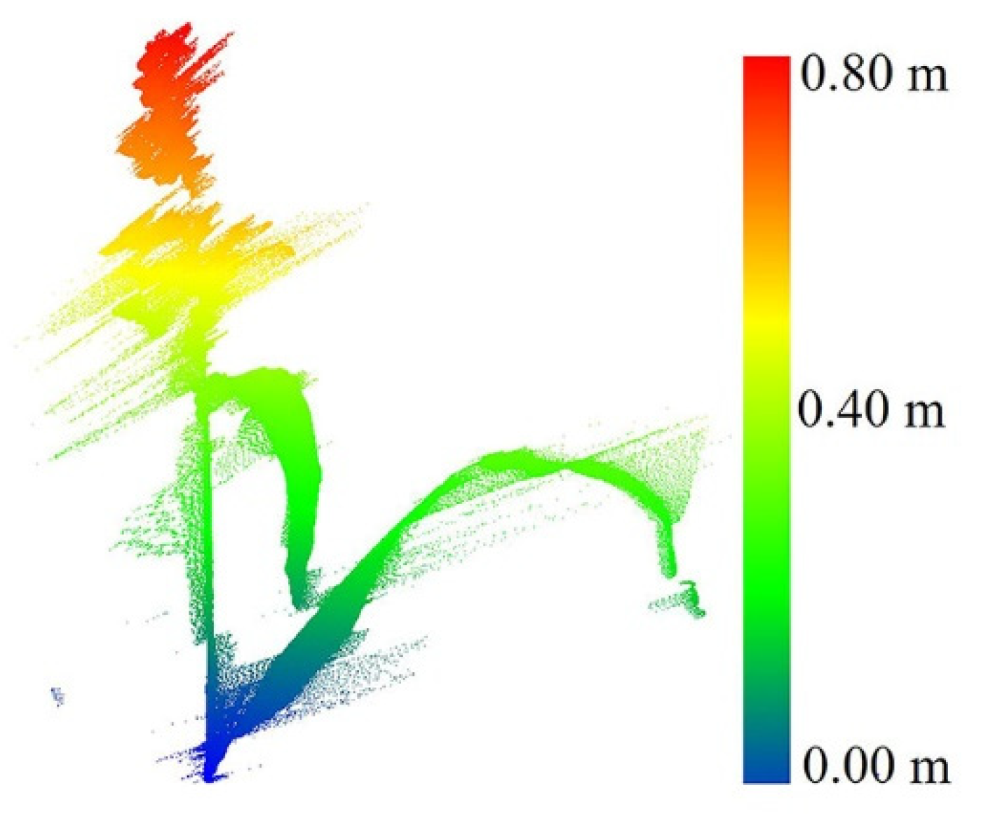
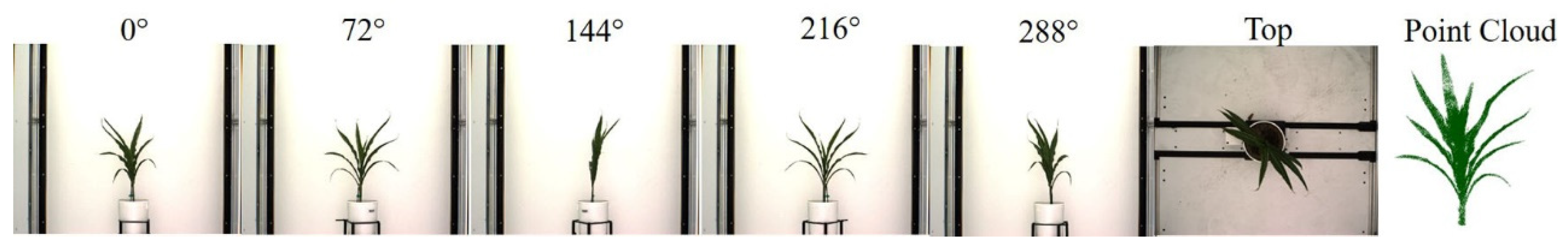
2.2.1. Stationary Scanning of Plants

A stationary LiDAR dataset was collected over a single sorghum plant in a greenhouse at Purdue University using a FARO terrestrial laser scanner. The FARO ${\mathit{Focus}}^{\mathit{3}\mathit{D}}$ X 330 single beam range is between 0.6 m and 330 m indoor or outdoor, with a range accuracy of ±2 mm. The total vertical field of view (FOV) and horizontal FOV are 300° and 360°, respectively. The point capture rate is ~122,000 points per second [27]. The average point distance (the distance of a point from its neighbors) in this dataset was 1.5 mm/10 m, when the scanner was located 2 m from the plant. The data were used to investigate the characteristics of the plant and associated noise and to explore geometric methods for outlier removal before applying them to field data. Figure 2 shows an example of a raw scan.

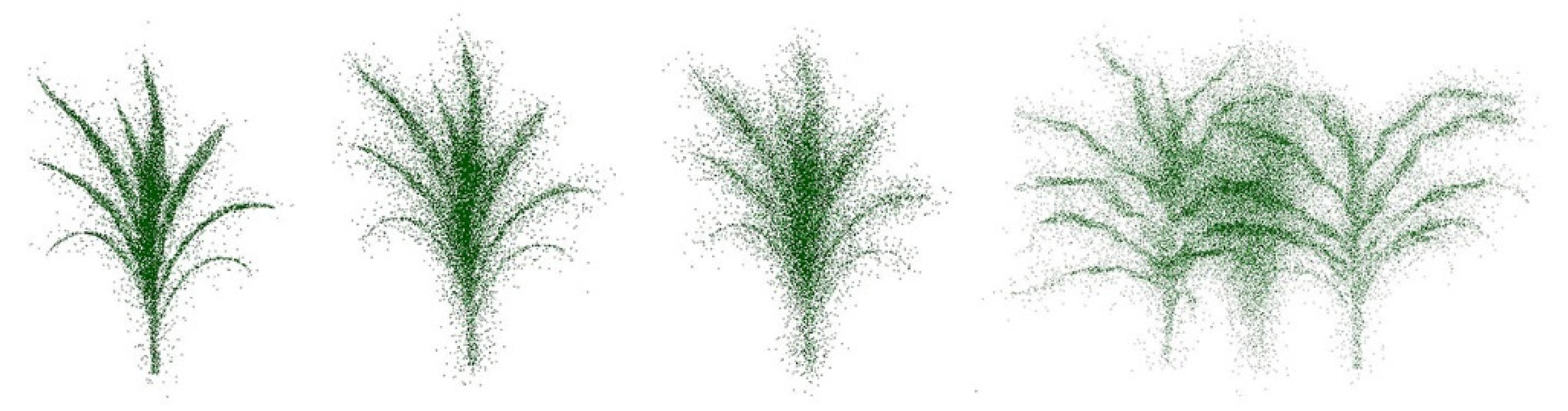
2.2.2. Image-Based Point Clouds for the Sorghum Training Dataset

A synthetic training set was developed to investigate the use of PointCleanNet for the outlier removal task. Collecting clean LiDAR data over plants in a farm environment without noise and outliers for the purpose of training is difficult and time-consuming, and is only possible at the edge of the field. In this study, the point cloud training dataset was obtained from overlapped RGB images on individual sorghum plants in a greenhouse. The images were acquired of plants at different stages of growth from 11 April 2018 to 19 May 2018 using a Basler piA 2400-17gc camera in a chamber in a controlled environment at the Crop in Silico project facility at the University of Nebraska, Lincoln. A set of images for each plant covered angles 0°, 72°, 144°, 216°, 288°, and a top view. Some datasets also included images at 36° and 216°. A volume carving method was used to generate the point cloud from the resulting images [28,29]. Figure 3 shows a sample of the overlapped images and the generated point cloud.

Thirty-five sets of generated point clouds from images were separated into 28 objects for training, and seven objects were chosen for validation. The outliers were generated by randomly adding Gaussian noise with a standard deviation of 20% of the shape’s bounding box diagonal in the dataset. The resulting training set had point clouds where 20%, 40, 50%, 70%, and 90% of the points were converted to outliers. To simulate the field scenario, some pairs and triplets of plants with different levels of outliers were joined and then added to the training set. Figure 4 illustrates some samples of the dataset.

2.2.3. LiDAR Remote Sensing Data

Three platforms collected LiDAR in the field for plant-breeding-related experiments in 2020. Two M600P UAVs were flown over the study area at altitudes of 20 and 40 m and speeds of 3–5 m/s. One UAV was equipped with a Velodyne VLP-Puck Lite and the other with a Velodyne VLP-32C. The Velodyne VLP-Puck LITE has 16 channels that are aligned vertically from −15° to +15°, thus resulting in a total vertical field of view (FOV) of 30°. The point capture rate in a single return mode is ~300,000 points per second. The range accuracy is typically ±3 cm, with a maximum measurement range of 100 m [30]. The Velodyne VLP-32C has 32 channels that are aligned vertically from −15° to +25°, in a total vertical FOV of 40°. The point capture rate in a single return mode is ~600,000 points per second. The range accuracy is typically ±3 cm, with a maximum measurement range of 200 m [31]. The UAVs were equipped with an integrated global navigation satellite system/inertial navigation system (GNSS/INS), Trimble APX-15v3, for direct georeferencing. Data were also acquired by a wheel-based system, a LeeAgra Avenger agricultural high-clearance tractor/sprayer with a custom boom and mounted sensors. It is referred to as the PhenoRover in these experiments. The boom is constructed from T-slot structural aluminum framing with a 2.75-m width, and the top of the boom can be raised to a maximum height of 5.5 m from the ground. The sensors mounted on the boom include a Headwall machine vision VNIR hyperspectral camera, an RGB camera, a Velodyne VLP-Puck Hi-Res, as well as a GNSS/INS navigation system. The VLP-Puck Hi-Res has a similar sensor specification to the VLP-Puck LITE. Its FOV is −10° to +10° [32]. The speed of the platform was 1.5 miles per hour in the field. Three-dimensional reconstruction for LiDAR is based on the point positioning equation (Equation (1)), as described in [33,34].

$$r_I^m=r_{b\left(t\right)}^m+R_{b\left(t\right)}^m{r}_{lu}^b+R_{b\left(t\right)}^m{R}_{lu}^b{r}_I^{lu\left(t\right)}$$

(1)

where $r_I^{lu\left(t\right)}$ is derived from raw LiDAR measurements at firing time and denotes the position of the laser beam footprint relative to the laser unit frame; $r_{b\left(t\right)}^m$ and $R_{b\left(t\right)}^m$ are the position and orientation information of the IMU body frame coordinate system relative to the mapping frame system at firing time t; $r_{lu}^b$ and $R_{lu}^b$ denote the lever arm and boresight rotation matrix relative to laser unit system and IMU body frame.

Figure 5 shows the platforms used for the 2020 experiments.

Table 2. Platforms’ and mounted sensors’ specifications.

Platform	Sensor	Unit	Description
UAV-1
	RGB camera	1	36.4 MP Sony Alpha 7R (ILCE-7R)
	LiDAR sensor	1	Velodyne VLP 16-Puck Lite-range accuracy of ±3 cm
	GNSS/INS	1	Trimble APX-15 v2
	Hyperspectral camera	1	Nano Hyperspectral (VNIR)
UAV-2
	RGB camera	1	36.4 MP Sony Alpha 7R (ILCE-7R)
	LiDAR sensor	1	Velodyne VLP 32-range accuracy of ±3 cm
	GNSS/INS	1	Trimble APX-15 v2
PhenoRover
	RGB camera	2	9.1 MP FLIR Grasshopper3 GigE
	Hyperspectral camera	1	Headwall Machine
	LiDAR sensors	1	Velodyne VLP-Puck Hi-Res
	GNSS/INS	1	Applanix POS-LV 125

details the UAV platforms and the PhenoRover, and their respective sensor specifications.

Table 3. LiDAR data and corresponding ground reference data in two experiments with associated DAS.

Experiment	Platform	Flying Height	Sowing Date	LiDAR Data Collection Date	DAS 1	Ground Reference Date	DAS 2
Maize	PhenoRover	N/A	05/12/2020	06/26/2020	45	06/29/2020	48
	UAV-2	20 m		07/07/2020	56	07/06/2020	55
	UAV-1	20 m		07/11/2020	60	07/13/2020	62
	UAV-2	20 m		07/11/2020	60	07/13/2020	62
	UAV-2	20 m		07/13/2020	62	07/13/2020	62
	PhenoRover	N/A		07/13/2020	62	07/13/2020	62
Sorghum	PhenoRover	N/A	05/13/2020	06/26/2020	44	06/29/2020	47
	UAV-2	20 m		07/07/2020	55	07/06/2020	54
	UAV-2	20 m		07/13/2020	61	07/13/2020	61
	PhenoRover	N/A		07/20/2020	68	07/20/2020	68
	UAV-2	20 m		07/20/2020	68	07/20/2020	68
	PhenoRover	N/A		07/24/2020	72	07/27/2020	75
	UAV-2	20 m		07/28/2020	76	07/27/2020	75

DAS ¹: DAS with respect to data collection data; DAS ²: DAS with respect to ground reference data.

summarizes the LiDAR data collection and the corresponding ground reference measurements in terms of days after sowing (DAS) relative to the data collection dates and ground reference measurements.

2.3. Methodology

The study included detection and removal of outliers from the experiments conducted in controlled facilities and the field. Data with low noise subsequent to outlier removal were considered as valid points. This section includes descriptions of the geometric approach for outlier removal and the deep learning PointCleanNet method for outlier removal.

2.3.1. Geometric Approach

In [5], isolated and non-isolated outliers occur in the point cloud. In this method, non-isolated outliers are first removed from the dataset based on majority voting. The normal to the fitting surface and curvature in the nearest neighbors of each point are calculated. The curvature describes the rate of change of a curve or plane at the chosen point. Small surface variation indicates that the neighborhood is regular; zero curvature implies a perfect plane. Points on sharp edges or at the extremum of curved surfaces may be classified as irregular points because of high curvature. Points are excluded via majority voting by regular points in the neighborhood of irregular points. This process is continued until all non-isolated points are detected and removed. In the experiments in the current research, not many points were transferred from irregular to regular because there were not many sharp surfaces in the point cloud geometry.

In [5], isolated points are removed by checking the intersection of the planes that are created on isolated points. This method can be applied to objects with a solid body. However, it does not perform well on complex objects with separate parts that have many intersecting planes, such as plants. To deal with this issue, we propose a region growing method based on the distance between points and the k-nearest neighbors (Figure 6) to detect and remove the sparse and isolated outlier points remaining in the dataset.

The points are structured with a k-d tree data structure, and the k-nearest neighbors to each point are determined within a defined radius. The points are assigned to the clusters based on the nearest neighbors. The clusters with common points are joined, and the cluster number is updated iteratively until no additional changes occur in the clusters. The clusters with fewer points than a specified threshold are removed as isolated outliers, and the remaining clusters are retained. In the end, the remaining points in the dataset are considered inliers. The workflow in Figure 7 shows the proposed procedure for outlier removal, with the component developed in [5] outlined.

As noted previously, the noise depends on both the characteristics of the system (e.g., platform type and sensor) and the objects being scanned (e.g., geometric complexity and size of the objects). Moreover, in the geometric approach, some parameters, including the best search radius, number of the nearest neighbor points, number of the points in the clusters, and thresholds related to point density and object complexity, are typically obtained by a grid search.

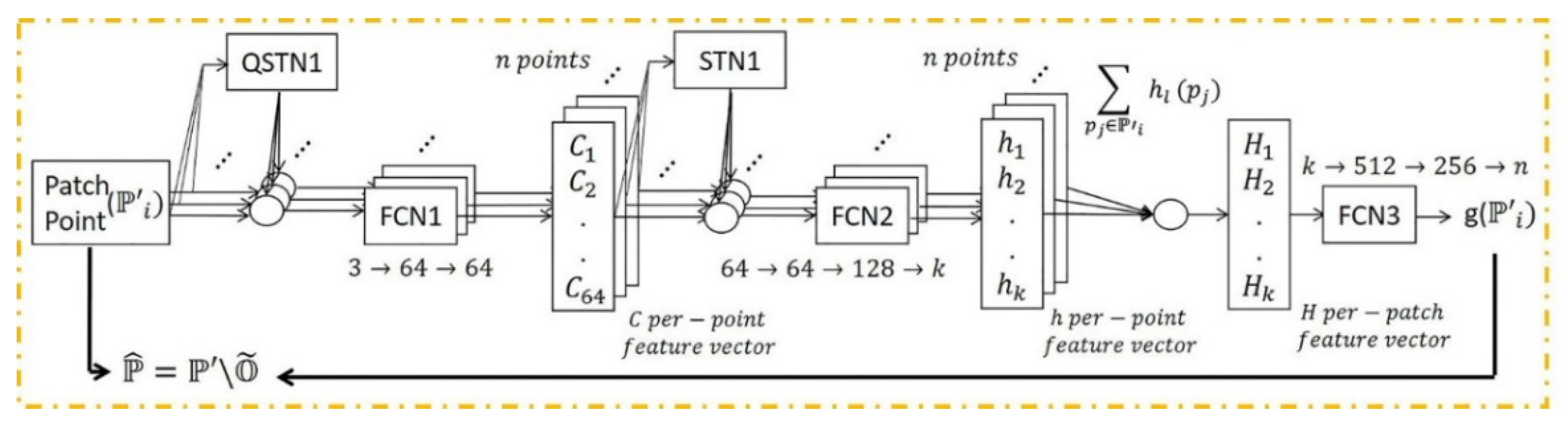
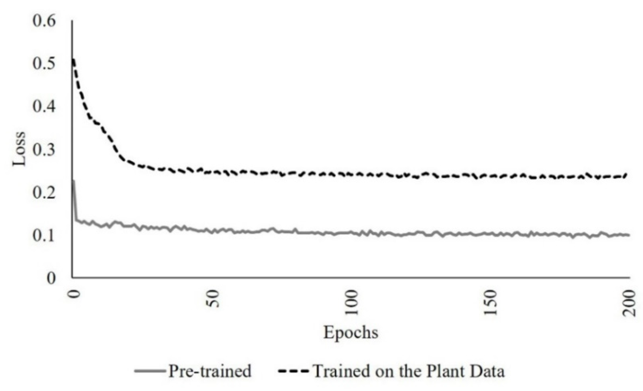
2.3.2. PointCleanNet-Based Outlier Removal

A deep learning framework may be more effective in removing outliers as the model trains iteratively using extensive quantities of training data with different types of objects in terms of shape, point density, and percentage of outliers. In this section, the PointCleanNet outlier removal is investigated with synthetic data. The details of the PointCleanNet network are included in [22]. Figure 8 illustrates the outlier removal architecture.

The network was first trained from scratch, and the loss was obtained using an augmented dataset that included the scanned data from a single sorghum plant, two and three joined plants with proportions of 20%, 40%, 50, 70%, 90% as outliers, using the default parameter values. The pre-trained model from [22], which is based on the point clouds of geometric and sculpture objects, was also lightly retrained by incorporating the plant data in the input using the default parameters. The loss obtained from the augmented pre-trained network was lower than from the self-trained network due to the limited diversity of the characteristics of the training data associated with the network trained from scratch on the plant data (Figure 9).

In terms of parameter tuning, the range of learning rate (0.00001 to 0.001 with a step size of 10) and patch radius size (0.01, 0.05, and 0.10 × bounding box diagonal) were evaluated using a grid search. The value of 0.0001 for learning rate and 0.05 × bounding box diagonal for patch radius size had the lowest loss, so the augmented pre-trained model with these setting parameters was selected as the final model.

The model was evaluated using the LiDAR dataset from the individual greenhouse plant with synthetic outliers and some of the synthetic datasets described in Section 2.2. The performance of the approach on these datasets was evaluated using the ${\mathrm{F}}_1$-score derived from the precision (Equation (2)) and recall (Equation (3)) of the test data; ${\mathrm{the} \mathrm{F}}_1$-score (Equation (4)) has a value between zero and one (zero indicates a poor result for the ${\mathrm{F}}_1$-score if either precision or recall is small). The best result is when there are no false outliers or false inliers in the result, with an ${\mathrm{F}}_1$-score of one.

$$\mathrm{Precision}=\frac{{\mathrm{T}}_{\mathrm{O}}}{{\mathrm{T}}_{\mathrm{O}}{+\mathrm{F}}_{\mathrm{O}}}$$

(2)

$$\mathrm{Recall}=\frac{{\mathrm{T}}_{\mathrm{O}}}{{\mathrm{T}}_{\mathrm{O}}{+\mathrm{F}}_{\mathrm{I}}}$$

(3)

$${\mathrm{F}}_1\text{-}\mathrm{score}=2 \times \frac{\mathrm{Precision} \times \mathrm{Recall}}{\mathrm{Precision}+\mathrm{Recall}}$$

(4)

where (${\mathrm{T}}_{\mathrm{O}}$) is the number of true outliers, (${\mathrm{F}}_{\mathrm{O}})$ is the number of false outliers, and (${\mathrm{F}}_{\mathrm{I}}$) is the number of false inliers. (A false inlier is defined as an outlier point that is falsely labeled as an inlier by the algorithm.)

The methods were also applied to the row crop data obtained from the UAV and PhenoRover platforms. The point density and canopy penetration varied across the platforms due to the LiDAR sensor models, the field of view, and mission characteristics (platform height and the overlap of successive flight lines). In this study, point density is investigated based on the flying height and model of the LiDAR sensor type.

Table 4. Ground point density for the HIPS maize experiment.

Date	Platform	Flying Height	DAS	Point Density (Points/m2)
11 July 2020	UAV-1	20 m	60	244
11 July 2020	UAV-2	20 m	60	617
13 July 2020	PhenoRover	N/A	62	1500

and

Table 5. Ground point density of sorghum over SbDivTc_Cal sorghum experiment.

Date	Platform	Platform Height	DAS	Point Density (Points/m2)
20 July 2020	UAV-2	20 m	68	500
20 July 2020	PhenoRover	N/A	68	1400

show the point density of the LiDAR over both fields based on the platform and flying height for example dates that were common between the two UAV platforms and UAV-2 and the PhenoRover.

It is extremely difficult to have an appropriate ground reference in row crop data for evaluating the outlier removal methods as many factors can affect the quality of the data, including the environmental conditions at the time of data collection, the density and arrangement of the plants, and the row geometry, as well as the platform and sensor. As a surrogate, the effect of the outlier removal algorithms on an estimated phenotyping parameter was estimated for the various experiments. Here, as noted earlier, the LAI was estimated before and after outlier removal over sorghum and maize experiments and used as the basis of comparison.

2.3.3. LAI Estimation

Geometric features were extracted from row crop LiDAR data, including the Laser Penetration Index [35], Vertical Complexity Index [36], mean height, standard deviation, and skewness [37], Cluster Area Plane Index (CAPI), 3rd quartile of height, and row-level plant volume (rows 2 and 3) within plots, as described in [38].

An optical indirect method based on an LAI-2200C plant canopy analyzer was used for ground reference. Empirical models, including stepwise multiple regression, partial least squared regression, and support vector regression with a radial basis function (RBF), were developed to represent the relationship between ground reference and LiDAR-based features. The data were randomly sampled as 75% and 25% to training and test sets, respectively, and ten-fold cross-validation was performed on the training set [38]. Results obtained for the original data and after outlier removal by the two approaches were evaluated based on the R² statistic and root mean squared error (RMSE) of the residuals (Equations (5) and (6)).

$${\mathrm{R}}^2 = 1 - \raisebox{1ex}{${\sum (\mathrm{y} - \hat{\mathrm{y}})}^2$}\!\left/ \!\raisebox{-1ex}{${\sum (\mathrm{y} - \stackrel{-}{\mathrm{y}})}^2$}\right.$$

(5)

$$\mathrm{RMSE} = {\left[\raisebox{1ex}{${\sum (\mathrm{y} - \hat{\mathrm{y}})}^2$}\!\left/ \!\raisebox{-1ex}{$n$}\right.\right]}^{\raisebox{1ex}{$1$}\!\left/ \!\raisebox{-1ex}{$2$}\right.}$$

(6)

where y and $\hat{\mathrm{y}}$ denote the LAI ground reference and estimated LAI, respectively, and $\stackrel{-}{\mathrm{y}}$ is the sample mean of the ground reference LAI; the number of samples is denoted by n.

3. Results and Discussion

Results obtained using the geometric method (modified [5] method) and the PointClearNet deep learning approach are presented in the following sections for data acquired in the control facilities and the field.

3.1. Geometric Outlier Removal from Individual Plants and Field Data

The point cloud obtained by the stationary scanner (see Section 2.2.1) was adequately dense to distinguish the plant structure. As noted in the previous section, outlier removal was achieved using two steps: removal of irregular points (bad points) connected to the main body of the plant and removal of sparse and isolated outliers. Figure 10 shows the original data with outliers and output from the two-step process. The search radius for the nearest neighbors was selected by grid search based on the point density (one cm), and the threshold for removing points in a cluster was six. The noise pattern seems to be associated with interference that tends to obscure the main body of the plant. While there is no control on this type of noise, the algorithm was able to remove these points effectively.

The synthetic datasets were generated from point clouds with three levels of outliers, 20%, 50%, and 70%, a radius search of one cm, and a cluster size threshold of 6. Three plant groupings with different levels of outliers, including (40%–90%–40%) and (70%–90%–70%), were evaluated using this method, as well with the radius search of two cm and a cluster size threshold of 10, which were each selected by grid search. Figure 11 and Figure 12 show the results and F₁-score of each of the synthetic datasets.

The precision score for the plant with 20% outliers (0.19) was lower than for the plant with 70% outliers (0.74). The total number of points was the same in both; the plant with 20% outliers had potentially more false outliers due to having more inlier points (80% inliers), thereby impacting the precision score.

The method was sensitive to radius search in a local neighborhood, as well as the number of points in the clusters, especially when the randomly distributed outliers were sparse. It is a trade-off between removing points as outliers and preserving points as the main structure of the plant. When precision was low, some true points were considered as outliers and removed, so parts of the plant structure were removed. Similarly, when the recall was low, some outliers remained in the main structure of the plant and were considered as true points. Thus, the gap between the points was smaller, but the number of outliers was larger. Additionally, when the points were distributed uniformly and were so sparse, the method could not discriminate the outliers from inliers.

For the HIPS maize experiment, data collected by the PhenoRover and UAV-2 were available. A radius search of 4 cm for the nearest neighbor was selected by a grid search, and the threshold for removing points in a cluster was 10 points for PhenoRover data; the radius search and the threshold for UAV data were 6 cm and 6 points, respectively. The radius search in UAV data was larger than for the PhenoRover data because the UAV point cloud was more sparse than the PhenoRover point clouds (Figure 13 and Figure 14).

The geometric method requires prior knowledge about the data in terms of point density and canopy penetration to select the thresholds, as well as trial-and-error experimentation to finalize the parameters. As shown visually in this section, the proposed geometric approach performed well on greenhouse data, where the plant was isolated from other objects, but the field data were much more difficult to denoise.

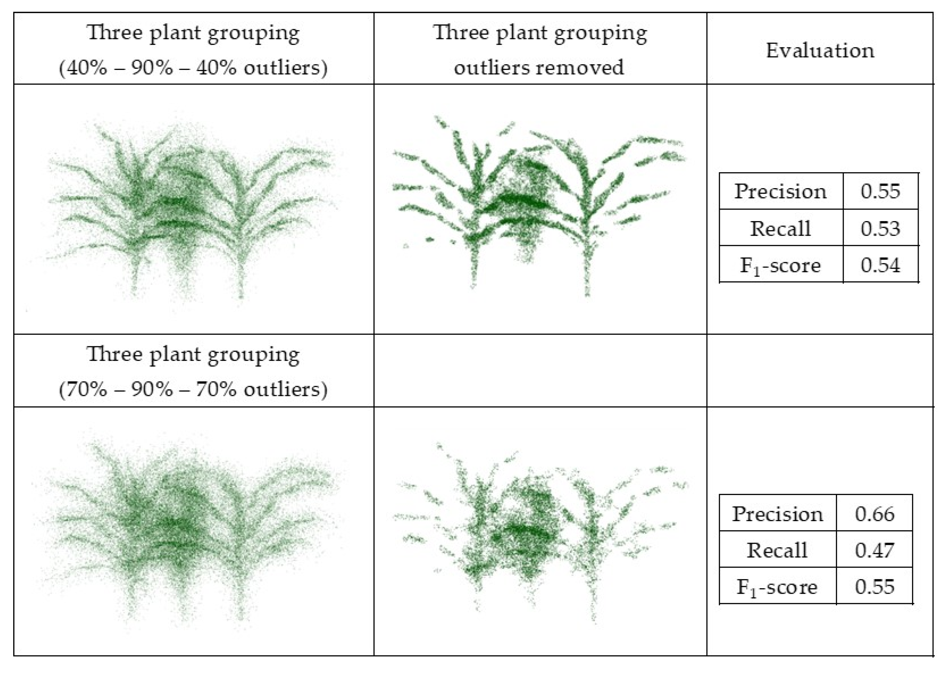
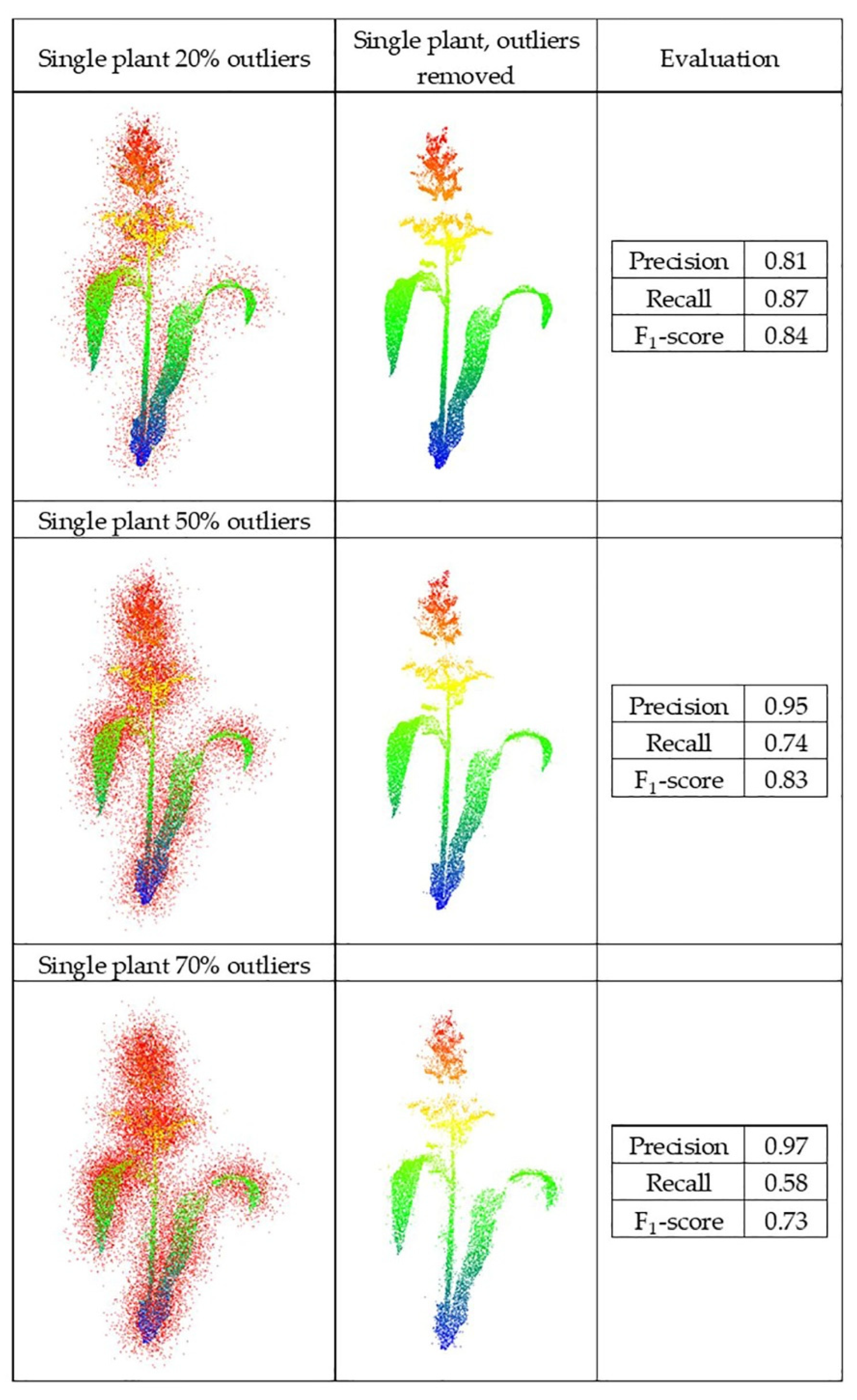
3.2. PointCleanNet Outlier Removal from Individual Plants and Field Data

The PointCleanNet method was applied to the point cloud single plants contaminated with multiple levels of outliers and investigated for row plants of sorghum and maize. The results obtained for both datasets are described and evaluated in this section.

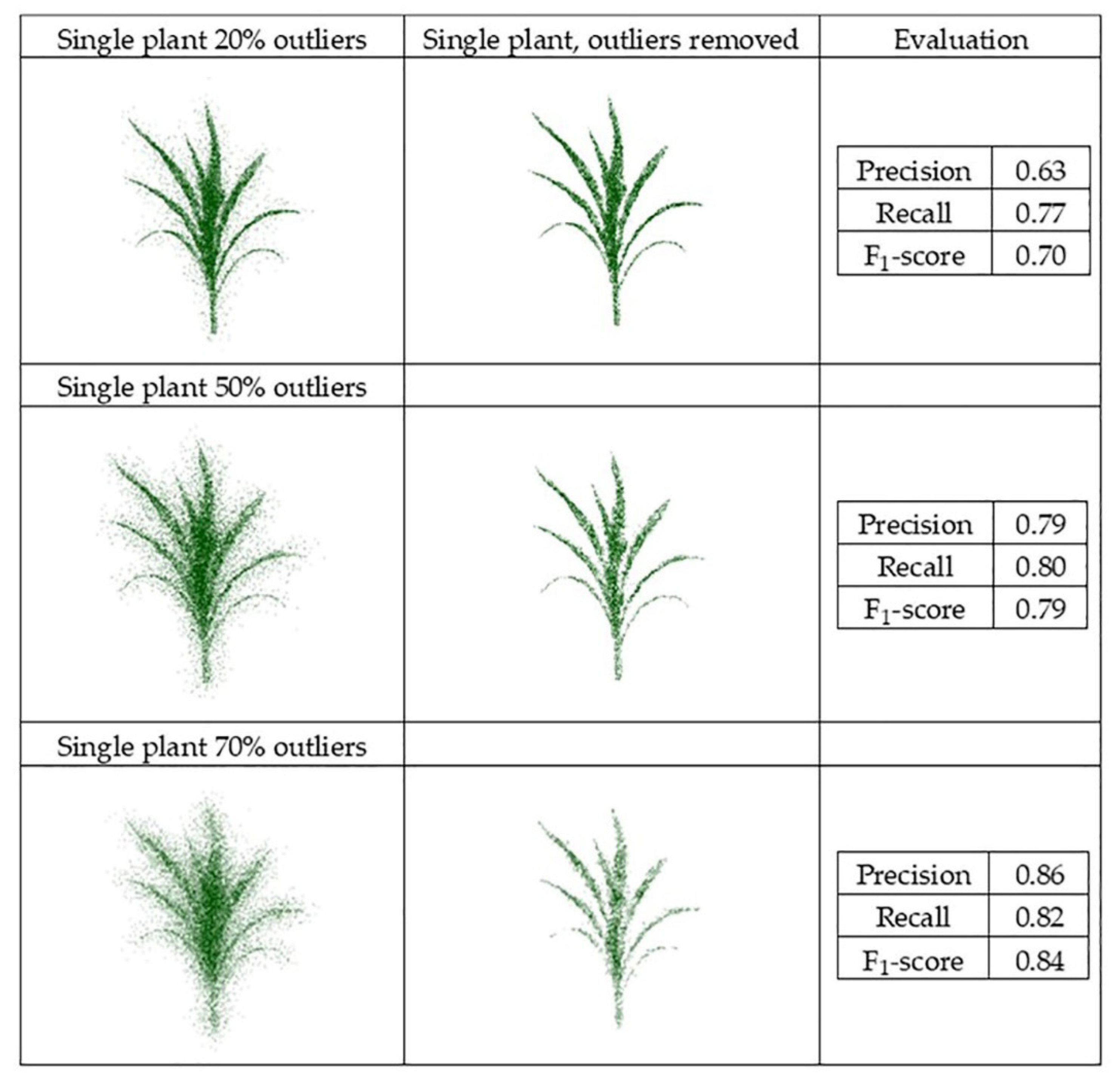
3.2.1. Single Plants

First, the dataset of the single sorghum plant from the greenhouse was contaminated with different levels of Gaussian outliers and used to evaluate the PointCleanNet-based on the F₁-score. The red points are outliers generated for each dataset (Figure 15).

After removal of the three levels of outliers, the structure of the plant was detectable, especially for the 20% and 50% experiments. However, when the outliers were 70% of the data for the single plant, the recall dropped significantly.

Datasets obtained from the generated point clouds were evaluated, and the F₁-score evaluated for the multiple scenarios (Figure 16 and Figure 17).

The F₁-score value from the individual plant with 70% outliers (0.84) was higher than the value from the plant with 20% outliers (0.70). This is because the number of false outliers in the 20% outlier case resulted in the value of precision of the plant with 20% outliers being lower than the plant with 70% outliers. As noted for the geometric noise removal approach, the total numbers of points in both datasets were the same; the plant with 20% outliers had more inliers (80%), which resulted in more false outliers. The two sets of three plant groupings with different levels of outliers had a similar F₁-score (0.79 and 0.80). The level of outliers was high in the middle plant in the grouping, and its structure was not detectable, while the structure of the plants on both sides was completely detectable as the level of outliers was lower. Comparing the deep learning results with the geometric results, it is clear that there are some missing parts of leaves in the geometric approach, while in the deep learning method, the leaves are complete and are visible.

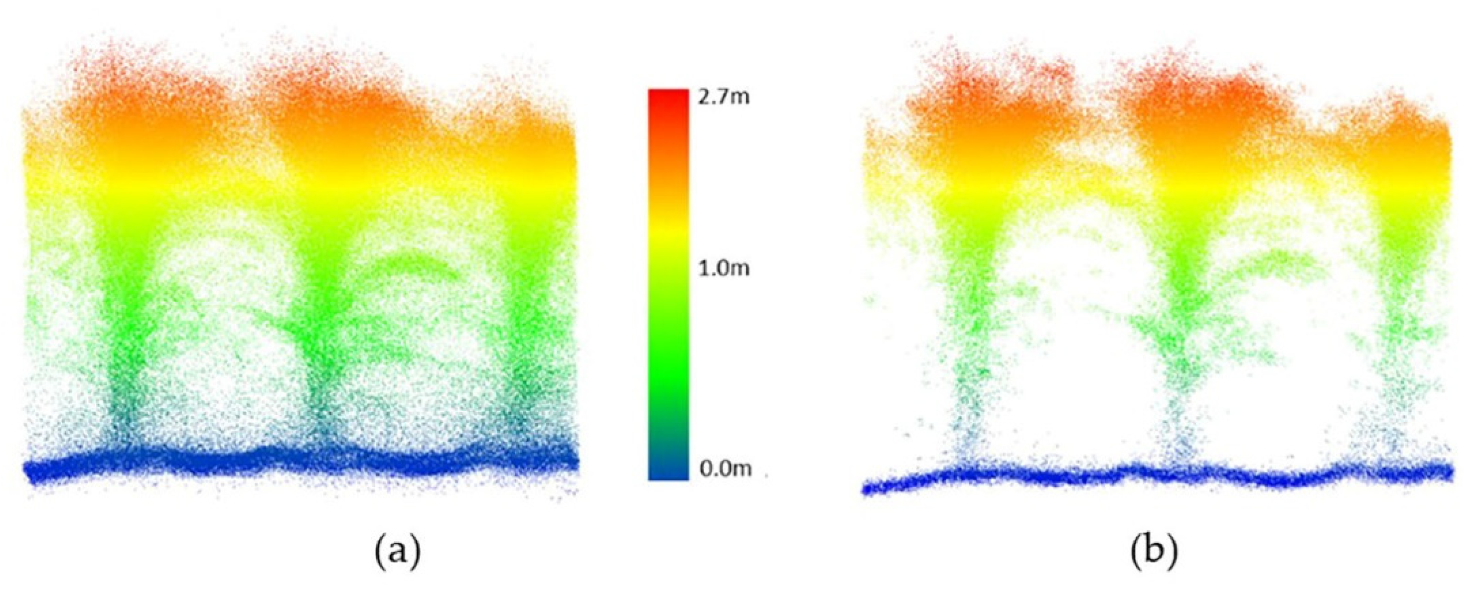
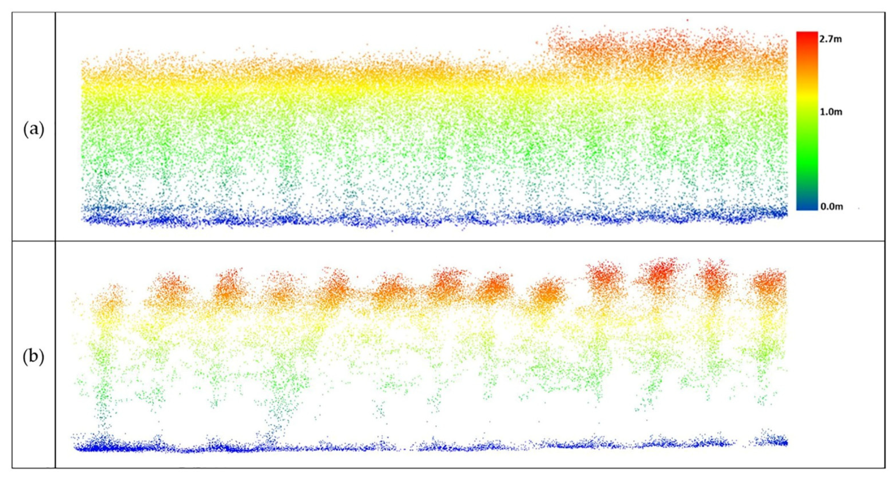
3.2.2. Outlier Removal from Maize and Sorghum Field Data

As noted previously, field data are planted densely (maize ~75,000 plants/hectare vs. sorghum ~200,000 plants/hectare) in multiple row plots, and the canopy closes between the rows as the growing season progresses. Figure 18, Figure 19, Figure 20 and Figure 21 show selected multi-row subsets of plots where outliers were removed from UAV-1, UAV-2, and PhenoRover data acquired over sorghum and maize.

When the UAV-1 acquired data at 20 m altitude with a VLP-Puck Lite (16 channels), penetration through the canopy was inadequate to identify the structure of plants beneath the top layer of the canopy, and plants from which outliers had been removed did not provide additional information (Figure 18).

The sample result in Figure 19 shows that the method removed outliers from UAV-2 data flying at 20 m, while many structure-related points were retained below the canopy. The resulting plant structure was more complete than the UAV-1 output shown in Figure 18. These results, while limited, indicate that significant increases in penetration are achieved at 20 m flying height, and that the VLP-32C has significantly better penetration than the 16-channel VLP-Puck Lite under these conditions.

While the PhenoRover point cloud data were more dense, there were additional sources of outliers, including the vibration of the boom and interaction of the platform with the plants during the later part of the growing season. The method removed some outliers but also removed some of the actual plant structure, although a significant part of the structure of the maize canopy was retained after denoising (Figure 20). The percentage of the removed points over maize was approximately 35–45% of the UAV data and 25% to 30% of the PhenoRover data.

Figure 21 shows a sample of sorghum data collected by UAV-2 flown at the altitude of 20 m.

Due to the complexity and density of sorghum, the point clouds remaining after denoising did not characterize the structure of the individual plants well. The percentage of the removed points over sorghum was approximately 40% to 50% of UAV data and 30% to 35% of the PhenoRover data.

In the deep learning method, when the plants (greenhouse and field) had very similar characteristics, and samples from all the cases were considered in the training set, there was no need to change any parameters when the shape, point density, and percentage of outliers varied within the bounds of these parameters. Although the results of synthetic plants from geometric and PointCleanNet methods are visually similar, PointCleanNet denoising yielded better results based on the F₁-score (e.g., 0.25 vs. 0.70 for 20% outliers on a single plant). Therefore, the PointCleanNet method was applied to all the plots in the field data (maize and sorghum) to remove the outliers, and the impact was evaluated based on estimated LAI. The results are discussed in Section 3.2.3.

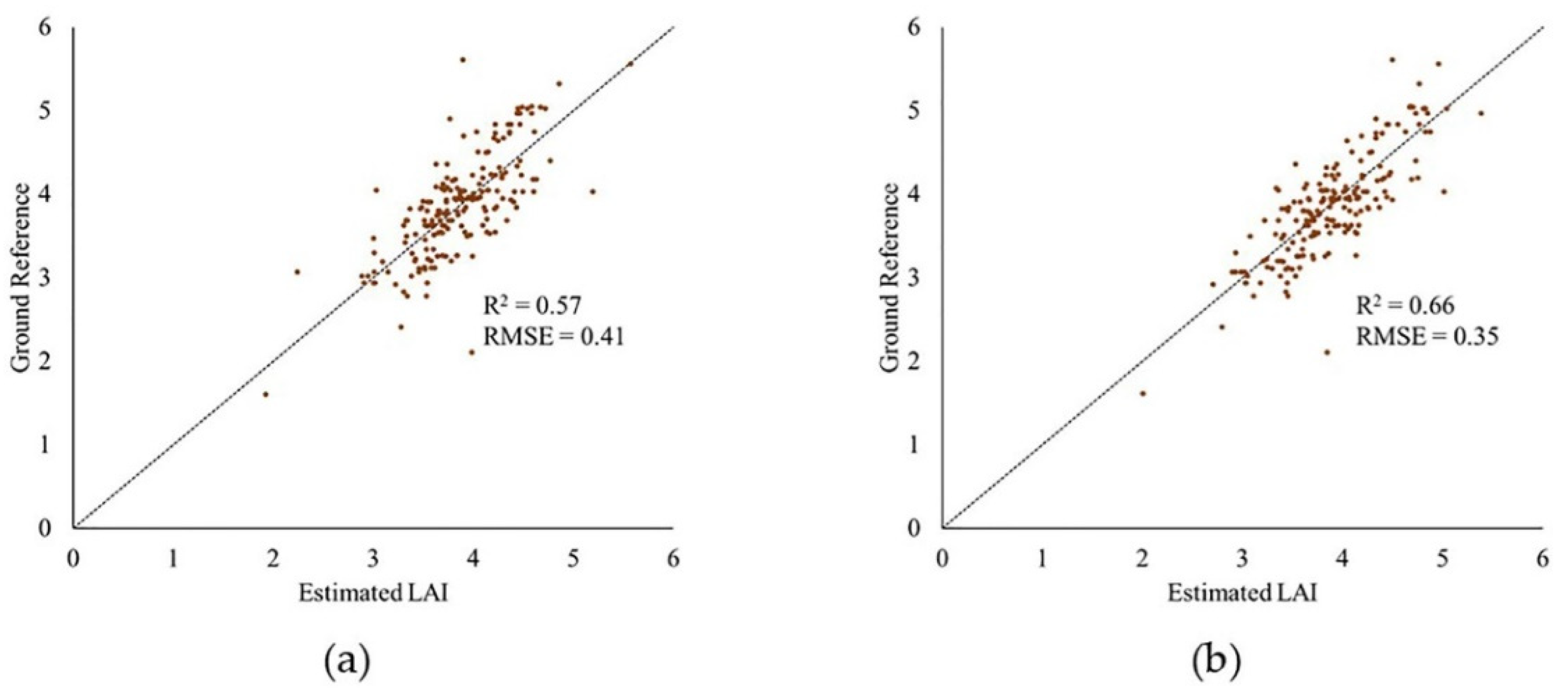
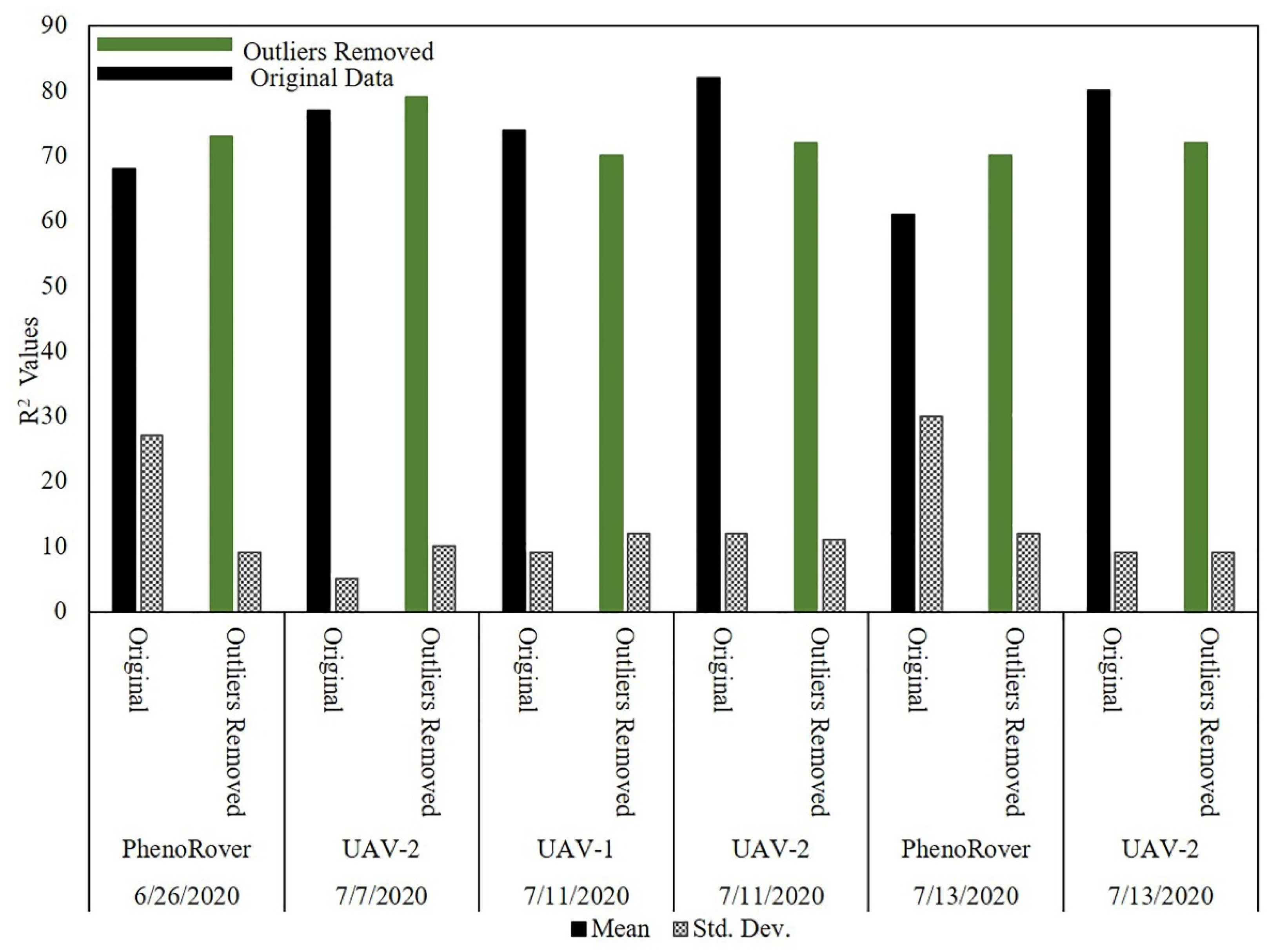
3.2.3. Impact of PointCleanNet Outlier Removal Method on LAI Estimation

The impact of outlier removal for both the UAV-2 (VLP-32C) flown at 20 m and PhenoRover data acquired over sorghum and maize fields is illustrated in this section relative to LAI using an SVR model. The impact of outlier removal on estimates of LAI was investigated for data acquired by UAV-2 and the Phenorover data using an SVR model with an RBF kernel. The mean and standard deviation of the respective R² values are shown in the bar chart in Figure 22.

After removing outliers from data, the R² value of the model increased for the PhenoRover for both 6/26/2020 and 7/24/2020 and was slightly lower for 7/20. The standard deviation of the estimated R² value was inconsistent for the PhenoRover. The impact of outlier removal was larger on 7/24/2020 in part because this day was windy (approximately 2.5 m/s) compared to other days with lower wind speeds. Figure 23 shows a sample plot of estimated LAI vs. the ground reference for 7/24/2020 PhenoRover data. In addition to improving the R² value, the RMSE decreased slightly after outlier removal.

The results showed that the effect of outliers on PhenoRover data is higher than the UAV data based on the R² value improvement after outlier removal. The R² values resulting from denoising the UAV data decreased, but the standard deviation of R² was also reduced. This implies that outlier removal reduced the anomalous data in terms of improving the LAI estimation, but that useful points were also removed. Overall, t-tests of the improvement related to the impact of outlier removal indicated that the change was not statistically significant at the 95% level (p-value = 0.79) based on the sample mean of R².

The impact of the PointCleanNet outlier removal algorithm was also evaluated on maize field data (HIPS) from UAVs at a flying height of 20 m and for the PhenoRover data (Figure 24).

The bar chart in Figure 24 shows that the R² value of the maize LAI predictions based on the three platforms was generally higher than for sorghum (e.g., values vary between 0.61 and 0.82, while R² values of sorghum LAI estimation varied from 0.51 to 0.70). The models based on data from which outliers had been removed by PointCleanNet had higher R² values for PhenoRover datasets (e.g., on 13 July, the R² value was improved from 0.61 to 0.70). The R² values from the original data also had a higher standard deviation of R² compared to the values for the UAV datasets. Similar to the sorghum models, the outliers did not have a significant impact on the LAI estimates for the UAV-based models. Although the maize is planted at a lower density, and the plant canopy is somewhat more open, the point density and penetration were still significantly lower for the UAVs than the PhenoRover. The p-value (0.78) of the t-test statistic indicates that the impact of the outlier removal method was also not statistically significant for maize at the 95% level for either the UAV-2 or the PhenoRover.

4. Conclusions

In this paper, a geometric method and a deep-learning-based approach (PointCleanNet) for outlier removal were investigated on a greenhouse plant and image-based point cloud plants. The impact of outlier removal was also investigated for plants grown in field plots. For the geometric method, outliers were categorized as non-isolated or isolated; non-isolated outliers were removed by the algorithm in [5], and isolated outliers were removed by extending this method. The geometric method requires specification of input parameters, including the radius search and number of points in a neighborhood of a point of interest. These parameters were sensitive to the distribution and density of the points in the dataset. When a platform is stationary, and the distribution of the points is uniform throughout the dataset, as in the example of the single plant in this study, finding the parameters is straightforward, as the density of points is adequate to detect the outliers. When the platform moves, the points are distributed sparsely. Coupled with the irregular shape of the objects, it is challenging for this method to remove the outliers. When the method was applied to maize and sorghum datasets acquired from UAVs and the PhenoRover wheeled vehicle, the geometric method did not perform well due to the extreme sparsity of points in the lower canopy. In the maize dataset, the structure of the plants became more clear and could be detected visually from both platforms. Although some outliers were removed from the sorghum dataset, the plant structure was not recognizable after outlier removal. This implies that the sparsity of the points in the datasets was a significant problem for this outlier removal approach.

The PointCleanNet deep learning framework was investigated for removing outliers from image-based point clouds derived from images in greenhouses and for field data. When the model was retrained using point clouds generated from overlapped images that were contaminated with different levels of simulated outliers, the loss was lower than when the model was trained solely on point clouds from plants. Based on the F-score, the network successfully removed different levels of outliers in the greenhouse data. PointCleanNet was also applied to both maize and sorghum data from field experiments, where the outliers included the impact of the complex plant structure and the movement of the platforms. LAI was estimated over field plots before and after PointCleanNet outlier removal using the sorghum and maize data from both platforms. The changes in the R² values of the models were not statistically significant improvements based on the t-test results. This may in part be due to the fact that LAI is based on the gap fraction, which relates to the distribution of points through the vertical space, not to overall structural characteristics, which had been improved by denoising, based on visualization. Although the p-values from t-test statistics (sorghum:0.79, maize:0.78) indicated that there was not a significant difference between results prior to and after outliers were removed, the R² values of estimated LAI from the PhenoRover improved both in terms of increasing the sample means and decreasing the standard deviations of R² (e.g., sorghum on 7/24/2020 before 0.57 and after 0.66). Based on these experiments, removal of outliers based on PointCleanNet appears to be justified for plant structures in greenhouses and for field data when the point density is greater than ~600 points per m2, as was the case for the low-altitude UAV and PhenoRover acquisitions, where canopy penetration was higher. It may also be useful for denoising LiDAR data acquired from a gantry. An indoor gantry would be close to the plants but would not interfere with them, unlike the PhenoRover in the field, or be subject to the weather. An outdoor gantry would provide an “intermediate” platform that would have improved penetration but not be subject to interference with the plants. It should be noted that outlier removal may prove more effective for the extraction of specific geometric features such as the number of leaves, leaf angle, etc., from the plants.

References

1. Deschaud, J.-E.; Goulette, F. Point Cloud Non Local Denoising Using Local Surface Descriptor Similarity. IAPRS 2010, 38, 109–114. [Google Scholar]
2. Fleishman, S.; Drori, I.; Cohen-Or, D. Bilateral Mesh Denoising. In Proceedings of the ACM Transactions on Graphics (TOG); ACM: New York, NY, USA, 2003; Volume 22, pp. 950–953. [Google Scholar]
3. Fan, H.; Yu, Y.; Peng, Q. Robust Feature-Preserving Mesh Denoising Based on Consistent Subneighborhoods. IEEE Trans. Vis. Comput. Graph. 2009, 16, 312–324. [Google Scholar]
4. Nurunnabi, A.; West, G.; Belton, D. Outlier Detection and Robust Normal-Curvature Estimation in Mobile Laser Scanning 3D Point Cloud Data. Pattern Recognit. 2015, 48, 1404–1419. [Google Scholar] [CrossRef] [Green Version]
5. Wang, Y.; Feng, H.-Y. Outlier Detection for Scanned Point Clouds Using Majority Voting. Comput.-Aided Des. 2015, 62, 31–43. [Google Scholar] [CrossRef]
6. Bengio, Y. Deep Learning of Representations for Unsupervised and Transfer Learning. JMLR Workshop Conf. Proc. 2012, 27, 17–36. [Google Scholar]
7. Lauzon, F.Q. An Introduction to Deep Learning. In Proceedings of the 2012 11th International Conference on Information Science, Signal Processing and their Applications (ISSPA), Montreal, QC, Canada, 2–5 July 2012; pp. 1438–1439. [Google Scholar]
8. Zhang, L.; Zhang, L.; Du, B. Deep Learning for Remote Sensing Data: A Technical Tutorial on the State of the Art. IEEE Geosci. Remote Sens. Mag. 2016, 4, 22–40. [Google Scholar] [CrossRef]
9. Cheng, G.; Yang, C.; Yao, X.; Guo, L.; Han, J. When Deep Learning Meets Metric Learning: Remote Sensing Image Scene Classification via Learning Discriminative CNNs. IEEE Trans. Geosci. Remote Sens. 2018, 56, 2811–2821. [Google Scholar] [CrossRef]
10. Ma, L.; Liu, Y.; Zhang, X.; Ye, Y.; Yin, G.; Johnson, B.A. Deep Learning in Remote Sensing Applications: A Meta-Analysis and Review. ISPRS J. Photogramm. Remote Sens. 2019, 152, 166–177. [Google Scholar] [CrossRef]
11. Petrovska, B.; Zdravevski, E.; Lameski, P.; Corizzo, R.; Štajduhar, I.; Lerga, J. Deep Learning for Feature Extraction in Remote Sensing: A Case-Study of Aerial Scene Classification. Sensors 2020, 20, 3906. [Google Scholar] [CrossRef]
12. Boulch, A.; Marlet, R. Deep Learning for Robust Normal Estimation in Unstructured Point Clouds. Comput. Graph. Forum 2016, 35, 281–290. [Google Scholar] [CrossRef] [Green Version]
13. Li, B.; Zhang, T.; Xia, T. Vehicle Detection from 3D Lidar Using Fully Convolutional Network. arXiv 2016, arXiv:1608.07916. [Google Scholar]
14. Agresti, G.; Schaefer, H.; Sartor, P.; Zanuttigh, P. Unsupervised Domain Adaptation for ToF Data Denoising with Adversarial Learning. In Proceedings of the IEEE Conference on Computer Vision and Pattern Recognition, Long Beach, CA, USA, 15–20 June 2019; pp. 5584–5593. [Google Scholar]
15. Agresti, G.; Minto, L.; Marin, G.; Zanuttigh, P. Deep Learning for Confidence Information in Stereo and Tof Data Fusion. In Proceedings of the IEEE International Conference on Computer Vision, Venice, Italy, 22–29 October 2017; pp. 697–705. [Google Scholar]
16. Cheng, X.; Zhong, Y.; Dai, Y.; Ji, P.; Li, H. Noise-Aware Unsupervised Deep Lidar-Stereo Fusion. In Proceedings of the IEEE Conference on Computer Vision and Pattern Recognition, Long Beach, CA, USA, 15–20 June 2019; pp. 6339–6348. [Google Scholar]
17. Qi, C.R.; Su, H.; Mo, K.; Guibas, L.J. PointNet: Deep Learning on Point Sets for 3D Classification and Segmentation. arXiv 2016, arXiv:1612.00593 [cs]. [Google Scholar]
18. Garcia-Garcia, A.; Orts-Escolano, S.; Oprea, S.; Villena-Martinez, V.; Garcia-Rodriguez, J. A Review on Deep Learning Techniques Applied to Semantic Segmentation. arXiv 2017, arXiv:1704.06857. [Google Scholar]
19. Jaderberg, M.; Simonyan, K.; Zisserman, A.; Kavukcuoglu, K. Spatial Transformer Networks. In Advances in Neural Information Processing Systems 28; Cortes, C., Lawrence, N.D., Lee, D.D., Sugiyama, M., Garnett, R., Eds.; Curran Associates, Inc.: Montreal, QC, Canada, 2015; pp. 2017–2025. [Google Scholar]
20. Ge, L.; Cai, Y.; Weng, J.; Yuan, J. Hand Pointnet: 3d Hand Pose Estimation Using Point Sets. In Proceedings of the IEEE Conference on Computer Vision and Pattern Recognition, Salt Lake City, UT, USA, 15–23 June 2018; pp. 8417–8426. [Google Scholar]
21. Guerrero, P.; Kleiman, Y.; Ovsjanikov, M.; Mitra, N.J. PCPNet Learning Local Shape Properties from Raw Point Clouds. Comput. Graph. Forum 2018, 37, 75–85. [Google Scholar] [CrossRef] [Green Version]
22. Rakotosaona, M.-J.; La Barbera, V.; Guerrero, P.; Mitra, N.J.; Ovsjanikov, M. POINTCLEANNET: Learning to Denoise and Remove Outliers from Dense Point Clouds. In Proceedings of the Computer Graphics Forum; Wiley Online Library: Hoboken, NJ, USA, 2019. [Google Scholar]
23. Lobell, D.B.; Thau, D.; Seifert, C.; Engle, E.; Little, B. A Scalable Satellite-Based Crop Yield Mapper. Remote Sens. Environ. 2015, 164, 324–333. [Google Scholar] [CrossRef]
24. Akinseye, F.M.; Adam, M.; Agele, S.O.; Hoffmann, M.P.; Traore, P.C.S.; Whitbread, A.M. Assessing Crop Model Improvements through Comparison of Sorghum (Sorghum bicolor L. Moench) Simulation Models: A Case Study of West African Varieties. Field Crop. Res. 2017, 201, 19–31. [Google Scholar] [CrossRef] [Green Version]
25. Blancon, J.; Dutartre, D.; Tixier, M.-H.; Weiss, M.; Comar, A.; Praud, S.; Baret, F. A High-Throughput Model-Assisted Method for Phenotyping Maize Green Leaf Area Index Dynamics Using Unmanned Aerial Vehicle Imagery. Front. Plant Sci. 2019, 10, 685. [Google Scholar] [CrossRef] [PubMed]
26. Fang, H.; Baret, F.; Plummer, S.; Schaepman-Strub, G. An Overview of Global Leaf Area Index (LAI): Methods, Products, Validation, and Applications. Rev. Geophys. 2019, 57, 739–799. [Google Scholar] [CrossRef]
27. FARO Focus3D X 330. Available online: https://faro.app.box.com/s/8ilpeyxcuitnczqgsrgp5rx4a9lb3skq/file/441668110322 (accessed on 27 September 2020).
28. Scharr, H.; Briese, C.; Embgenbroich, P.; Fischbach, A.; Fiorani, F.; Müller-Linow, M. Fast High Resolution Volume Carving for 3D Plant Shoot Reconstruction. Front. Plant Sci. 2017, 8, 1680. [Google Scholar] [CrossRef] [PubMed] [Green Version]
29. Gaillard, M.; Miao, C.; Schnable, J.C.; Benes, B. Voxel Carving Based 3D Reconstruction of Sorghum Identifies Genetic Determinants of Radiation Interception Efficiency. Plant Direct 2020, 4, e00255. [Google Scholar] [CrossRef] [PubMed]
30. Velodyne VLP-Puck LITE. Available online: http://www.mapix.com/wp-content/uploads/2018/07/63-9286_Rev-H_Puck-LITE_Datasheet_Web.pdf (accessed on 1 November 2021).
31. Velodyne VLP-32C. Available online: http://www.mapix.com/wp-content/uploads/2018/07/63-9378_Rev-D_ULTRA-Puck_VLP-32C_Datasheet_Web.pdf (accessed on 1 November 2021).
32. Velodyne VLP-Puck Hi-Res. Available online: http://www.mapix.com/wp-content/uploads/2018/07/63-9318_Rev-E_Puck-Hi-Res_Datasheet_Web.pdf (accessed on 1 November 2021).
33. Zhou, T.; Hasheminasab, S.M.; Habib, A. Tightly-Coupled Camera/LiDAR Integration for Point Cloud Generation from GNSS/INS-Assisted UAV Mapping Systems. ISPRS J. Photogramm. Remote Sens. 2021, 180, 336–356. [Google Scholar] [CrossRef]
34. Ravi, R.; Habib, A. Fully Automated Profile-Based Calibration Strategy for Airborne and Terrestrial Mobile LiDAR Systems with Spinning Multi-Beam Laser Units. Remote Sens. 2020, 12, 401. [Google Scholar] [CrossRef] [Green Version]
35. Richardson, J.J.; Moskal, L.M.; Kim, S.-H. Modeling Approaches to Estimate Effective Leaf Area Index from Aerial Discrete-Return LIDAR. Agric. For. Meteorol. 2009, 149, 1152–1160. [Google Scholar] [CrossRef]
36. Pope, G.; Treitz, P. Leaf Area Index (LAI) Estimation in Boreal Mixedwood Forest of Ontario, Canada Using Light Detection and Ranging (LiDAR) and WorldView-2 Imagery. Remote Sens. 2013, 5, 5040–5063. [Google Scholar] [CrossRef] [Green Version]
37. Nie, S.; Wang, C.; Dong, P.; Xi, X.; Luo, S.; Zhou, H. Estimating Leaf Area Index of Maize Using Airborne Discrete-Return LiDAR Data. IEEE J. Sel. Top. Appl. Earth Obs. Remote Sens. 2016, 9, 3259–3266. [Google Scholar] [CrossRef]
38. Nazeri, B. Evaluation of Multi-Platform LiDAR-Based Leaf Area Index Estimates Over Row Crops. Ph.D. Thesis, Purdue University Graduate School, West Lafayette, IN, USA, 2021. [Google Scholar]
Figure 1. Plot variety layout: (a) SbDivTc calibration panel and (b) HIPS.
Remotesensing 13 04445 g001
Figure 2. Original single sorghum plant collected in the greenhouse.
Remotesensing 13 04445 g002
Figure 3. Overlapped images acquired for generating point clouds.
Remotesensing 13 04445 g003
Figure 4. Left to right: samples with 20%, 50%, and 70% outliers; three-plant grouping.
Remotesensing 13 04445 g004
Figure 5. (a) PhenoRover platform with RGB/LiDAR/Hyperspectral/GNSS/INS sensors, (b) UAV-2 with RGB/LiDAR/GNSS/INS sensors.
Remotesensing 13 04445 g005
Figure 6. Region growing clustering steps: (a) point cloud; (b) initial clustering; (c) finding common points in two close clusters; (d) connecting and joining two clusters.
Remotesensing 13 04445 g006
Figure 7. The workflow of geometric outlier detection in two steps; non-isolated outliers were removed by the [5] method, and isolated outliers were removed by a clustering proposed method.
Remotesensing 13 04445 g007
Figure 8. PointCleanNet outlier removal architecture; , ^ , and O ˜ denote a dataset contaminated with outliers as input, the dataset after outlier removal, and outliers, respectively. FCN and (Q)STN are the Fully Connected and (Quaternion) Spatial Transformer Networks. The input is a patch point, and output is a label for each point related to its status as an outlier [22].
Remotesensing 13 04445 g008
Figure 9. Pre-trained vs. the network trained on the plant data loss in 200 epochs (the number of iterations).
Remotesensing 13 04445 g009
Figure 10. (a) Original LiDAR data with natural outliers. (b) Coarse-level outlier removal from a sorghum plant. Arrows show the residual outliers from this step. (c) Result of removal of residual outliers with two different views.
Remotesensing 13 04445 g010
Figure 11. Geometric method outlier removal for a synthetic point cloud.
Remotesensing 13 04445 g011
Figure 12. Geometric method outlier removal on joint point cloud generated from three sorghum plants grouping.
Remotesensing 13 04445 g012
Figure 13. UAV-2 LiDAR data of maize (DAS:60). (a) Original data, (b) point cloud after outlier removal.
Remotesensing 13 04445 g013
Figure 14. PhenoRover LiDAR data over maize (DAS:62). (a) Original data, (b) point cloud after outlier removal.
Remotesensing 13 04445 g014
Figure 15. Outlier removal on individual plant LiDAR.
Remotesensing 13 04445 g015
Figure 16. PointCleanNet outlier removal for a point cloud based on a single plant.
Remotesensing 13 04445 g016
Figure 17. PointCleanNet outlier removal on joint point cloud generated from three sorghum plants grouping.
Remotesensing 13 04445 g017
Figure 18. Data from UAV-1 at 20 m altitude over maize (DAS: 60). (a) Original data, (b) outlier removal with PointCleanNet.
Remotesensing 13 04445 g018
Figure 19. Data from UAV-2 at the altitude of 20 m over maize (DAS: 60). (a) Original point cloud perpendicular to the direction of the rows; (b) results of outlier removal using PointCleanNet.
Remotesensing 13 04445 g019
Figure 20. PhenoRover LiDAR data of maize (DAS:62). (a) Original data, (b) outlier removal using PointCleanNet.
Remotesensing 13 04445 g020
Figure 21. UAV-2 LiDAR data of sorghum (DAS:68). (a) Original data, (b) outlier removal using PointCleanNet.
Remotesensing 13 04445 g021
Figure 22. Estimates of LAI for original data and after PointCleanNet-based outlier removal from data acquired by the UAV and PhenoRover.
Remotesensing 13 04445 g022
Figure 23. Plot of estimated LAI vs. ground reference: (a) original and (b) with outliers removed from PhenoRover data (24 July 2020) using PointCleanNet method.
Remotesensing 13 04445 g023
Figure 24. Maize LAI estimation on original and datasets with PointCleanNet outlier removal during the growing season on UAV and PhenoRover.
Remotesensing 13 04445 g024