1. Introduction
Video synthetic aperture radar (Video-SAR) provides high-resolution SAR images at a faster frame rate, which is conducive to the continuous and intuitive observation of ground moving targets. Due to this advantage, Video-SAR brings about important applications in SAR moving target tracking [
1]. Since the Sandia National Laboratory (SNL) of the United States first obtained high-resolution SAR images in 2003 [
2], many scholars have investigated the problem of moving target tracking in Video-SAR [
3,
4,
5,
6,
7]. However, due to different angles of illumination, the scattering characteristics of moving targets change with the movement of the platform. Worse still, it is difficult to track a moving target directly because the imaging results of the moving target usually shift from their true position.
Fortunately, shadow is caused by the ground being blocked by the moving target. Due to the absence of energy reflection, shadows appear at the real position of the moving target in the SAR image, with the advantage of a constant grayscale [
8]. Therefore, shadow-aided moving target tracking has become a hot topic in Video-SAR. In recent years, many scholars have worked on shadow-aided moving target tracking in Video-SAR [
9,
10,
11]. Wang et al. [
9] fully considered the constant grayscale of shadows and used data multiplexing to achieve moving target tracking. Zhao et al. [
10] applied the saliency-based detection mechanism and used spatial–temporal information to achieve moving target tracking in Video-SAR. Tian et al. [
11] utilized the dynamic programming-based particle filter to achieve the track-before-detect algorithm in Video-SAR. However, the features used by these traditional methods are usually simple, which leads to the problem of the background being similar to the shadow, meaning it cannot be easily distinguished. Deep learning methods then emerged to solve shadow tracking due to their high accuracy and fast speed advantages [
12,
13,
14,
15,
16]. Ding et al. [
12] presented a framework for shadow-aided moving target detection using deep neural networks, which applied a faster region-based convolutional neural network (Faster-RCNN) [
13] to detect shadows in a single frame and used a bi-directional long short-term memory (Bi-LSTM) [
14] network to track the shadows. Zhou et al. [
15] proposed a framework by combining a modified real-time recurrent regression network and a newly designed trajectory smoothing long short-term memory network to track shadows. Wen et al. [
16] proposed a moving target tracking method based on the dual Faster-RCNN, which combined the shadow detection results in SAR images and the range-Doppler (RD) spectrum to suppress false alarms for moving target tracking in Video-SAR.
However, arbitrary target-of-interest (TOI) tracking is a challenge for the above methods. In this paper, we define TOI as a specific target in a video that one wants to track. TOI refers to the shadow to be tracked in Video-SAR. The reasons why arbitrary TOI tracking is a challenge are as follows: First, these methods are all based on appearance features, such as shape and texture. These methods need to train a large number of labeled training samples to extract appearance features, and the training samples must include the TOI. However, when we track an arbitrary TOI, it is impractical to collect samples of all categories for training because of the targets’ diversity and arbitrariness. Moreover, it takes extensive work and material resources to label a large number of SAR images. Therefore, these methods are both impractical and costly when tracking an arbitrary TOI in Video-SAR.
Thus, we propose a novel guided anchor Siamese network (GASN) for arbitrary TOI tracking in Video-SAR. First, the key of GASN lies in the idea of similarity learning, which learns a matching function to estimate the degree of similarity between two images. After training using a large number of paired images, the learned matching function in GASN, given an unseen pair of inputs (TOI in the first frame as the template, and the subsequent frame as the search image), is used to locate the area that best matches the template. As GASN only relies on the template information, which is independent of the training data, it is suitable for tracking arbitrary TOIs in Video-SAR. Additionally, a guided anchor subnetwork (GA-SubNet) in GASN is proposed to suppress false alarms and to improve the tracking accuracy. GA-SubNet uses the location information of the template to obtain the location probability in the search image, and then it selects the location with a probability greater than the threshold to generate sparse anchors, which can exclude false alarms. To improve the tracking accuracy, the anchor that more closely matches the shape of the TOI is obtained by GA-SubNet through adaptive prediction processing.
The main contributions of our method are as follows:
We established a new network GASN, which trains a large number of paired images to build a matching function to judge the degree of similarity between two inputs. After similarity learning, GASN matches the subsequent frame with the initial area of the TOI in the first frame and returns the most similar area as the tracking result.
We constructed a GA-SubNet embedded in GASN to suppress false alarms, as well as to improve the tracking accuracy. By incorporating the prior information of the template, our proposed GA-SubNet can generate sparse anchors that match the shape of the TOI the most.
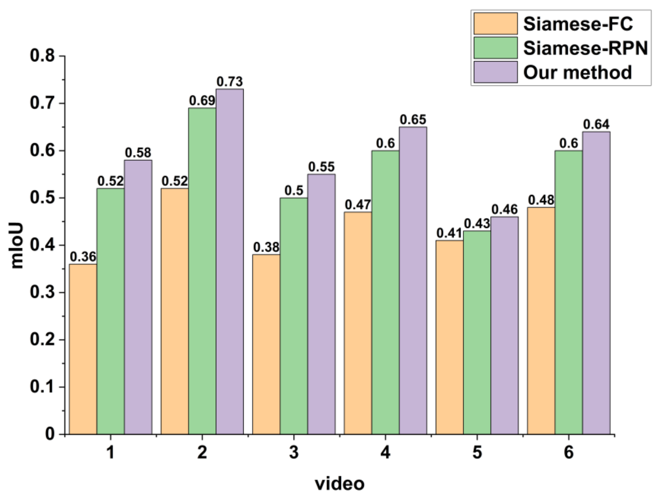
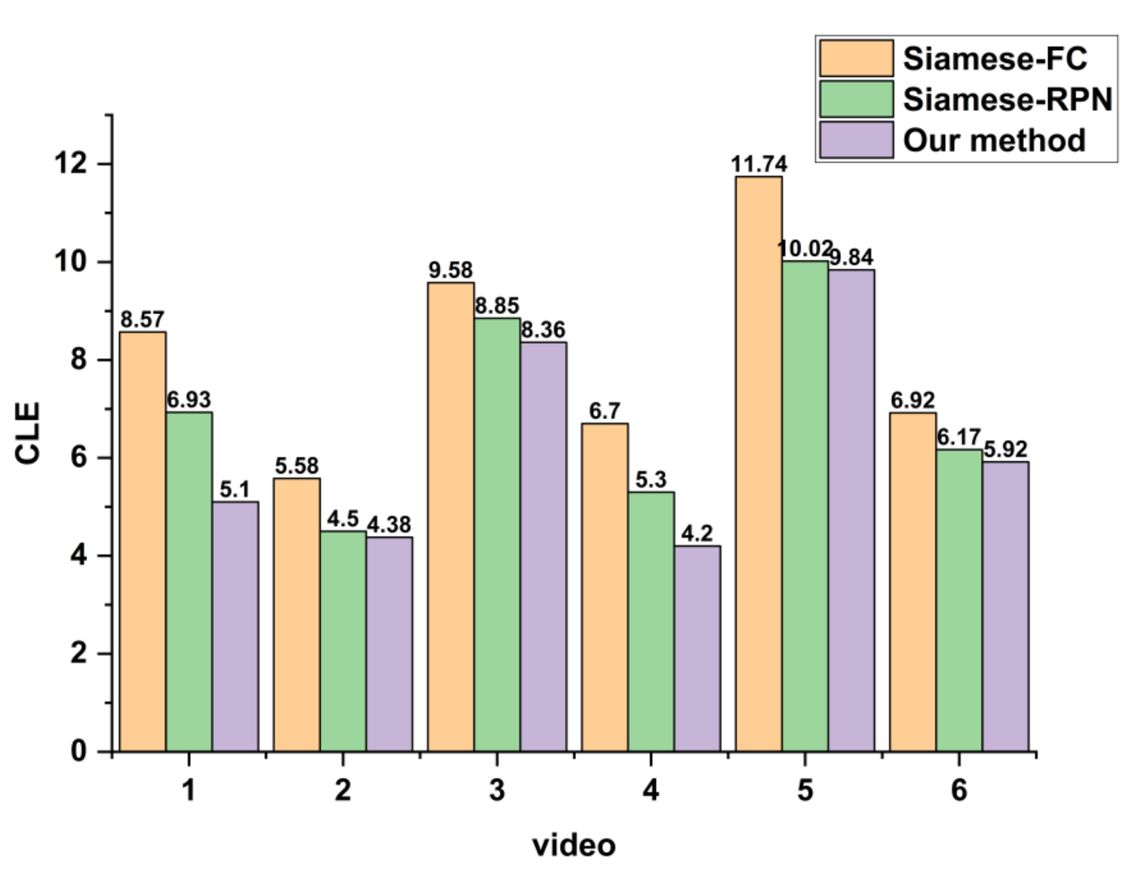
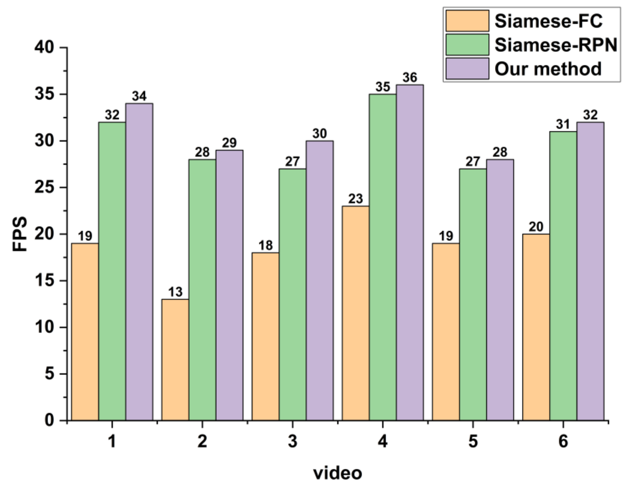
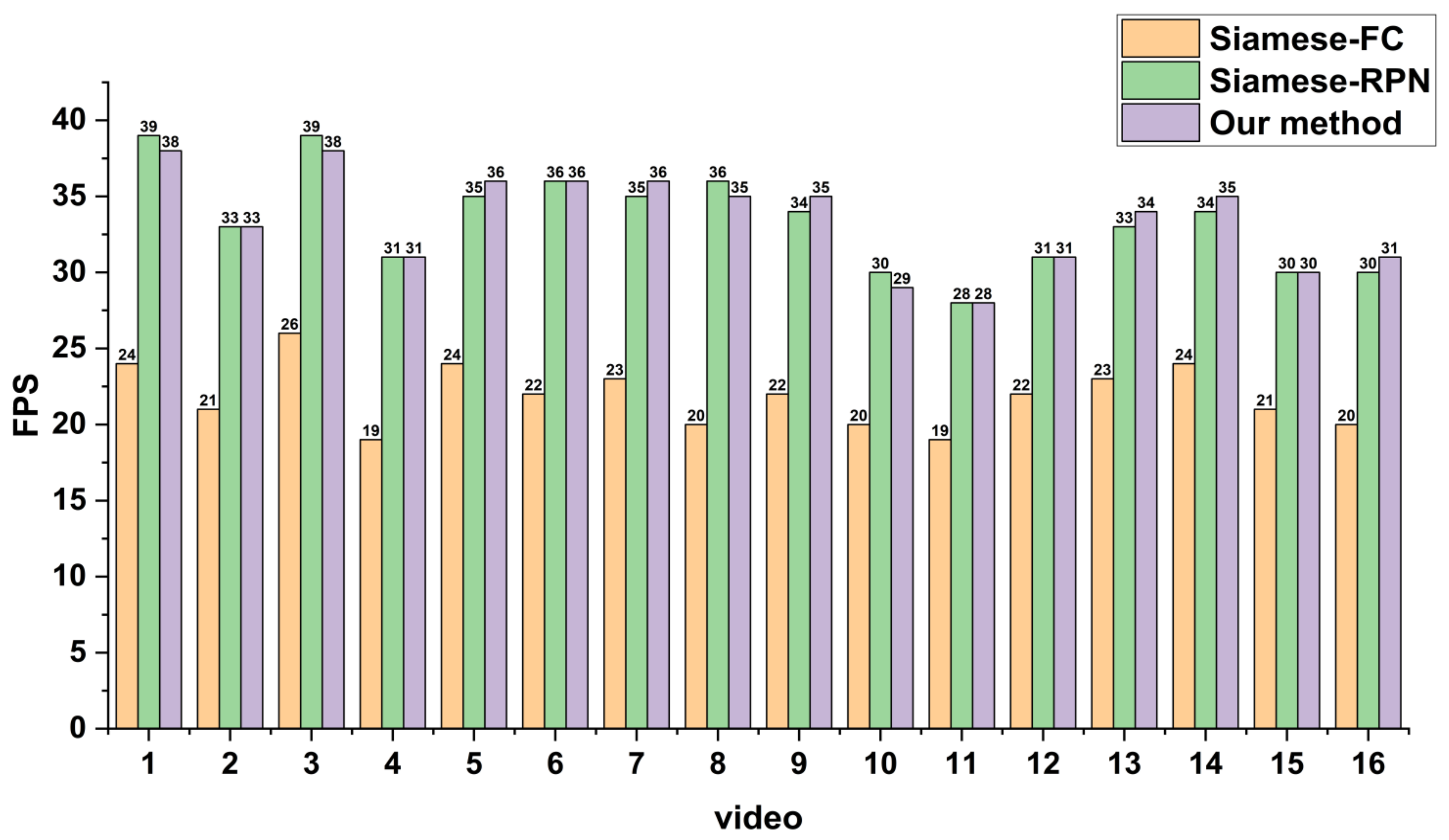
To verify the validity of the proposed method, we performed experiments on simulated and real Video-SAR data. The results showed that the tracking accuracy of the proposed network is 60.16% on simulated Video-SAR data, 4.55% and 16.49% higher than the two deep learning methods Siamese-RPN [
17] and Siamese-FC [
18], as well as 18.36% and 28.95% higher than the two traditional methods MOSSE [
19] and KCF [
20], respectively. Meanwhile, the tracking accuracy is 54.68% on real Video-SAR data, which is higher than the other four methods by 1.93%, 13.08%, 14.70%, and 25.04%, respectively. This demonstrates that our method can achieve accurate arbitrary TOI tracking in Video-SAR.
The rest of this paper is organized as follows:
Section 2 introduces the methodology, including the network architecture, preprocessing, and tracking processes.
Section 3 introduces the experiments, including the simulated and real data, the implementation details, the loss function, and the evaluation indicators.
Section 4 introduces the simulated and real Video-SAR data tracking results.
Section 5 discusses the research on pre-training and robustness and the ablation experiment.
Section 6 provides the conclusion.
2. Methodology
2.1. Network Architecture
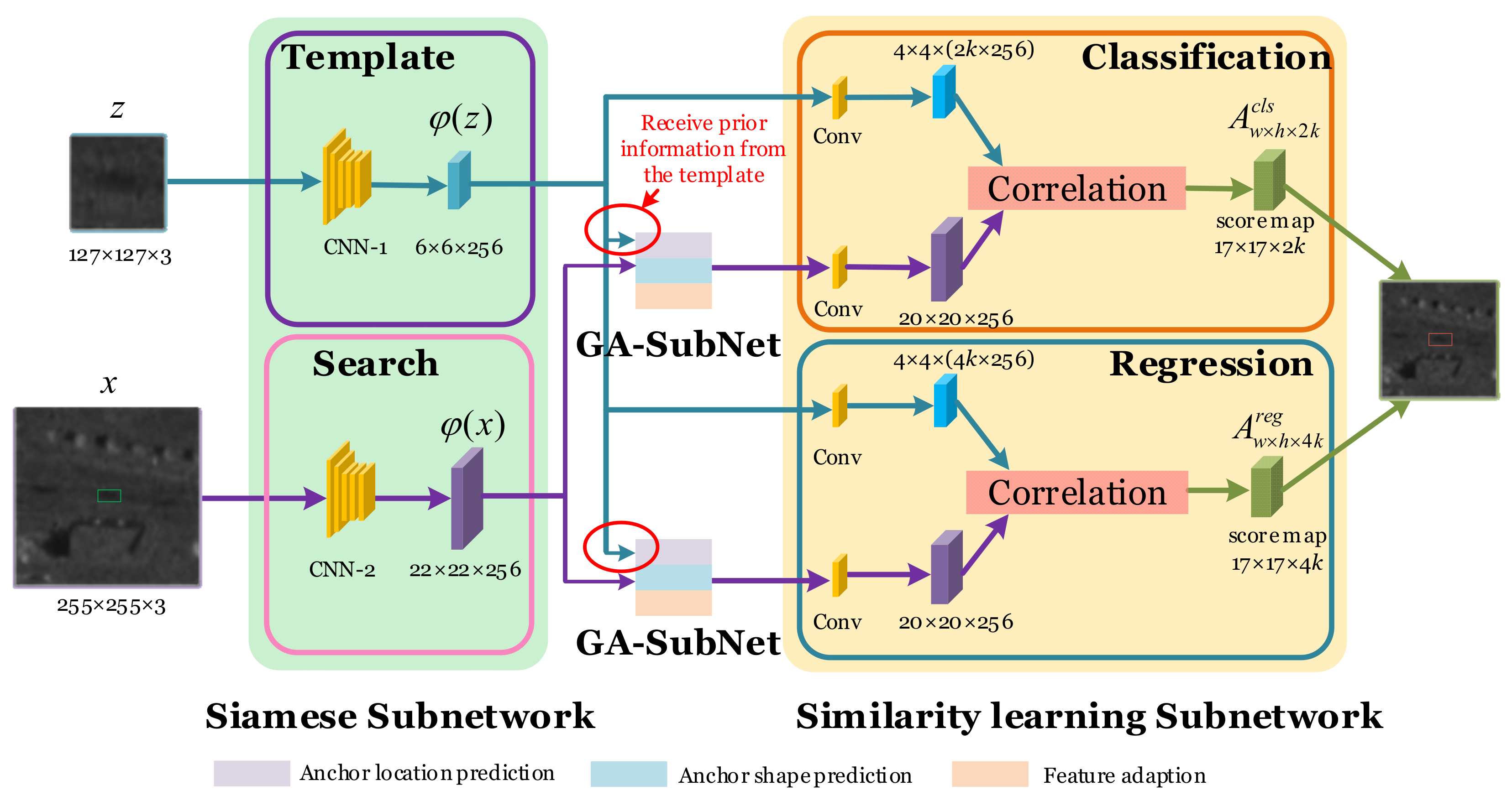
Figure 1 shows the architecture of GASN for arbitrary TOI tracking in Video-SAR, including the Siamese subnetwork, GA-SubNet, and the similarity learning subnetwork. GASN is based on the idea of similarity learning, which compares a template image
z to a search image
x and returns a high score if the two images depict the same target.
To prepare for similarity learning, the Siamese subnetwork consists of a template branch and a search branch. The two branches apply identical transformation φ to each input, and the transformation φ can be considered as feature embedding. Then, similarity learning can be expressed as f (z, x) = g (φ(z), φ(x)), where the function g is a similarity metric. To suppress false alarms, GA-SubNet receives the prior information from the template to pre-determine the general location and shape of the TOI in the search image using anchors. When tracking an arbitrary TOI that is different from the training sample, we can use the ability of similarity learning to find the TOI in the next frame by providing the template information of said TOI, such as the position and shape. The similarity learning subnetwork is divided into two branches, one for the classification of the shadow and background, and the other for the regression of the shadow’s location and shape. In both branches, the similarity between the shadow template and the search area is calculated, and then the target with the maximum similarity to the template of the TOI is chosen as the tracking result.
GASN always uses the previous frame as the template image and the current frame as the search image. After testing the whole SAR image sequence in such a way, GASN can achieve arbitrary TOI tracking in Video-SAR. In the following, we introduce the three subnetworks of GASN in detail in the order of implementation.
2.1.1. Siamese Subnetwork
The Siamese subnetwork (marked as the green region in
Figure 1) [
21,
22] uses CNN for feature embedding. CNN uses different convolutional kernels for multi-level feature embedding of the image. Therefore, compared to the traditional manual features, the features embedded by the Siamese subnetwork are more representative and can describe the TOI better. To obtain the common features of the previous and current frames, the Siamese subnetwork is divided into a template branch (marked with a purple box) and a search branch (marked with a pink box), and the parameters of CNN-1 and CNN-2 in both branches are shared to ensure the consistency of features. The input of the template branch is the TOI area in the previous frame (denoted as
z), and the input of the search branch is the search area in the current frame (denoted as
x). See
Section 2.2 for details about the preprocessing of the input images. For convenience, we denote the output feature maps of the template and search branches as
φ(
z) and
φ(
x).
2.1.2. GA-SubNet
After obtaining the feature maps, we established a GA-SubNet to suppress false alarms and improve the tracking accuracy. The specific architecture of GA-SubNet is shown in
Figure 2, including anchor location prediction, anchor shape prediction, and feature adaptation. In the following, we introduce the three modules of GA-SubNet in detail in the order of implementation.
The purple region in
Figure 2a is the anchor location prediction, i.e., the prediction of the location of the anchor containing the center point of a shadow. First, the input to GA-SubNet is two feature maps, one for the template (marked with a blue cube) and the other for the search area (marked with a purple cube). To obtain the prior information of the template that is independent of the training data, the feature map of the template is used as the kernel to convolute the feature map of search area
F1, so that the score of each location of the output represents the probability that the corresponding location is predicted to be the shadow. Then, the sigmoid function is used to obtain the probability map as shown in the blue box in
Figure 2a. After this, the position whose probability exceeds the preset threshold is chosen to be the location of the predicted anchor (marked with a red circle). To learn more information about the shadow, similar to [
17], the empirical threshold was chosen as 0.7.
The blue region in
Figure 2b is the anchor shape prediction, i.e., the prediction of the anchor shape that better conforms to the shape of a shadow. First, the uniform arbitrary preset anchor shapes are generated (marked with blue boxes) at each location obtained from the anchor location prediction; i.e., several anchor shapes are arbitrarily set at each location, but the anchor shape setting in sparse locations is uniform. The preset anchor shape with the largest IoU with the shadow’s ground truth (marked with a green box) is predicted as the leading shape (marked with an orange box). IoU is defined by Equation (1), where
P denotes the preset anchor shapes, and
G denotes the shadow’s ground truth.
The leading shape of the anchor is still set arbitrarily and may differ significantly from the shadow’s ground truth. To make the IoU larger, the offset between the leading shape and the shadow’s ground truth at each location is calculated. After continuously optimizing the offsets using the loss function (described in
Section 3.3), the best anchor shape can be obtained (marked with a white box), which better conforms to the shape of the shadow.
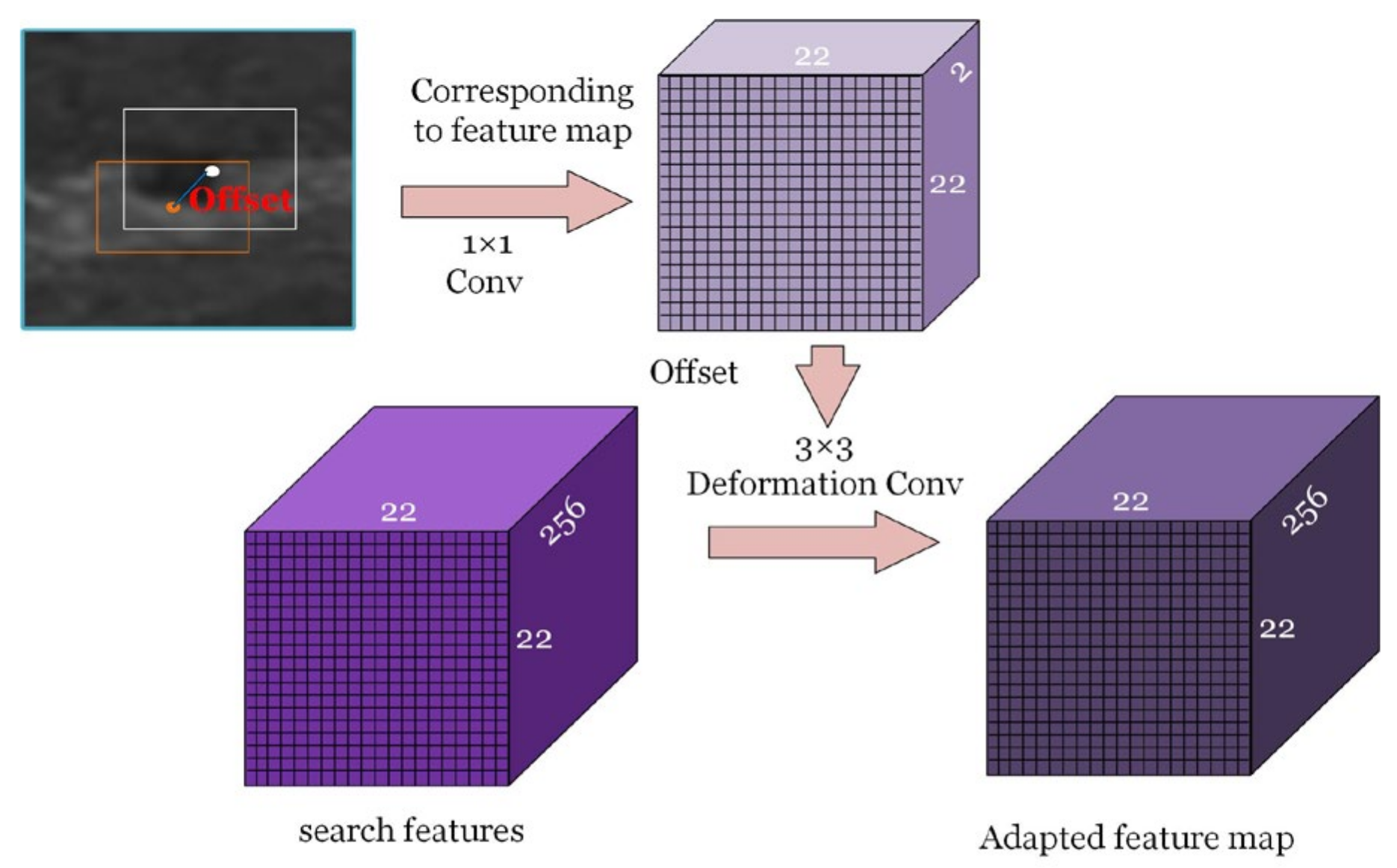
The orange region in
Figure 2c is the feature adaptation, i.e., the adaptation of the feature map and the SAR image. Because the feature map is obtained by multi-layer convolution of the SAR image, there is a certain correspondence between the feature map and the SAR image; i.e., the leading shape of the anchor in the SAR image corresponds to a specific region in the feature map. However, the leading shape of the anchor at each location is optimized adaptively in the anchor shape prediction, resulting in areas with the same shape in the feature map, corresponding to the areas with different shapes in the SAR image. Therefore, feature adaptation is necessary to satisfy the correspondence between the feature map and the SAR image to ensure the accuracy of tracking. First, 1 × 1 convolution is used to calculate the offset between the leading shape and the best shape. Then, 3 × 3 deformed convolution is applied [
23,
24] based on this offset to the original feature map
F1 of the search area. Finally, the feature map
F2 is obtained for adaptation to the SAR image for the best anchor shape.
2.1.3. Similarity Learning Subnetwork
After obtaining the sparse anchors that better conform to the shadows’ shape, the similarity learning subnetwork (marked with a yellow region in
Figure 1) is used for classification and regression. The similarity learning subnetwork consists of a classification branch (marked with an orange box in
Figure 1) for distinguishing the shadow from the background and a regression branch (marked with a blue box in
Figure 1) for predicting the location and shape of the shadow. First, in both branches, to reduce the calculation complexity for subsequent similarity learning, a feature map 6 × 6 of
φ(
z) is reduced to 4 × 4 and a feature map 22 × 22 of
φ(
x) is reduced to 20 × 20 by using the convolutions (marked with yellow cubes in
Figure 1). In addition, the channel of
φ(
z) is adjusted to 2
k × 256 for the foreground and background classification in the classification branch. The channel of
φ(
z) is adjusted to 4
k × 256 for determining the location and shape of the shadow in the regression branch.
k is the number of anchors, 2
k represents the probability of the foreground and background for each anchor, and 4
k represents the location (
x,
y) and shape (
w,
h) of the shadow.
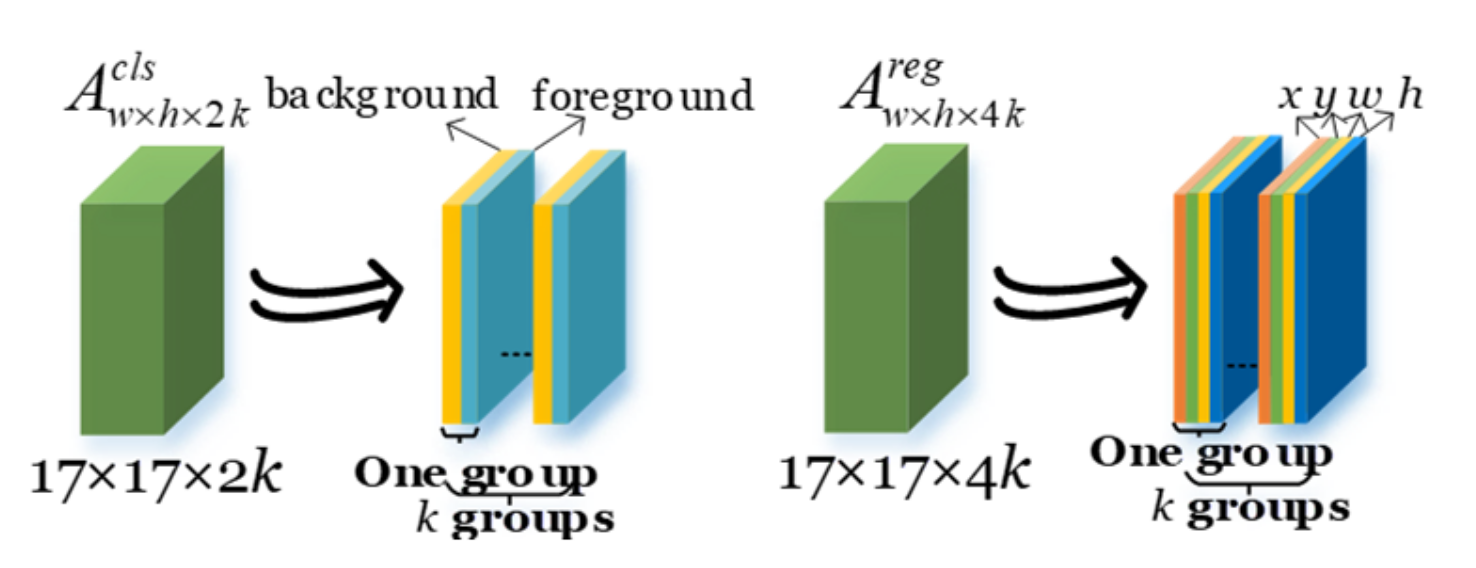
As shown in Equation (2), the similarity learning subnetwork applies pairwise correlations (marked with red rectangles in
Figure 1) to calculate the similarity metric, in which the similarity map
is for classification and
is for regression.
and
represent the classification and regression, respectively, and
denotes the convolution operation. We show the feature composition of
and
in
Figure 3.
is divided into
k groups, and each group contains two feature maps, which indicate the foreground and background probabilities of the corresponding anchors. The anchor is the foreground if the probability of the foreground is higher; otherwise, it is the background. Similarly,
is divided into
k groups, and each group contains four feature maps (
x,
y,
w, and
h), which indicate the similarity metric between the corresponding anchor and the template. According to the highest similarity, the optimal location and the shape of the shadow are obtained.
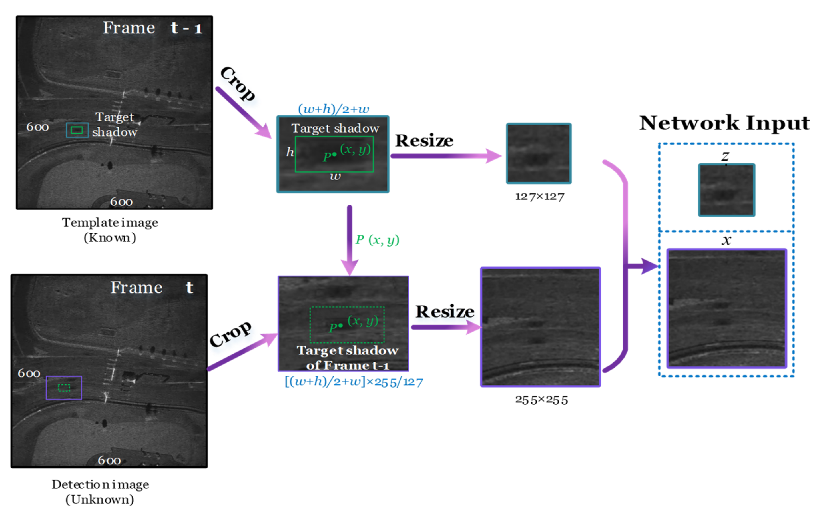
2.2. Preprocessing
For all images of Video-SAR to have the same feature dimensions, preprocessing is required before entering GASN. As shown in
Figure 4, the input of GASN is a pair of adjacent images in the SAR image sequence. The shadow template is a 127 × 127 area centered on the center (
x,
y) of the shadow in frame
t-1. Similar to the image preprocessing in [
17], we cropped an ((
w +
h) × 0.5 +
w, (
w +
h) × 0.5 +
h) area in frame
t-1 centered on (
x,
y) and then resized it to 127 × 127, where (
w,
h) is the boundary of the shadow. Here, (
x,
y,
w, and
h) are known in the training stage, while in the testing stage, the parameters represent the prediction results of the previous frame. Because the template size of all existing methods is 127 × 127 [
17,
18], to ensure the rationality of the comparison, we chose 127 × 127 as the template size. The search area is centered on the center of the shadow in frame
t, and we cropped an (((
w +
h) × 0.5 +
w) × 255/127, ((
w +
h) × 0.5) +
h) × 255/127) area and then resized it to 255 × 255. This area is larger than the shadow’s template to ensure that the shadow is always included in the search area.
2.3. Tracking Process
The whole process of TOI tracking based on GASN is shown in
Figure 5. The details are as follows.
Step 1: Input Video-SAR image sequence.
As shown in
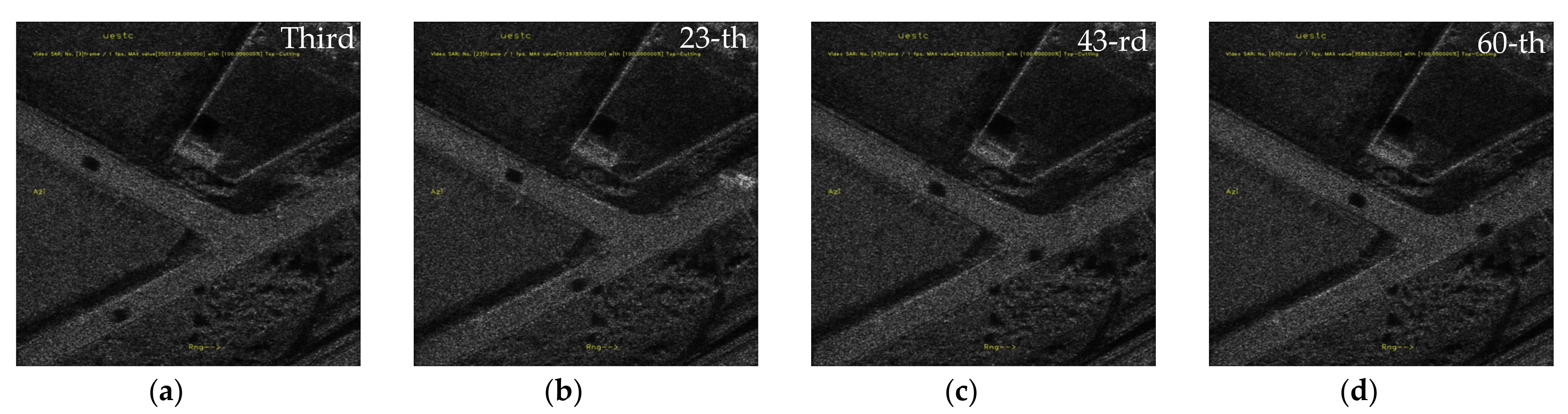
Figure 6a,
N is the number of frames of the input video. For easy observation, we marked the shadow to be tracked with a green box.
Step 2: Preprocessing SAR images.
For all images of Video-SAR to have the same feature dimensions, we need to crop and resize them. As described in
Section 2.2, the shadow in frame
t-1 is resized to 127 × 127 as the template, and frame
t is resized to 255 × 255 as the search area, as shown in
Figure 6b.
x,
y,
w, and
h represent the center and boundary of the prediction results in the previous frame. Unlike the RGB three-channel optical images, the SAR images are gray; therefore, all three channels are assigned to the same gray value to use the pre-trained weights. Applying models trained on three-channel RGB images to one-channel radar images has been carried out in several published literatures [
10,
12,
15], and the results in
Section 5.3 show that it is reasonable to do so.
Step 3: Embed features by the Siamese subnetwork.
After obtaining the template and search areas, the Siamese subnetwork embeds features to better describe the TOI. The Siamese subnetwork is divided into a template branch and a search branch, and the parameters of CNN-1 and CNN-2 in the two branches are shared to ensure the consistency of the features. The template branch outputs 6 × 6 × 256 as the feature map of the template, and the search branch outputs 22 × 22 × 256 as the feature map of the search area, which are shown in
Figure 6c.
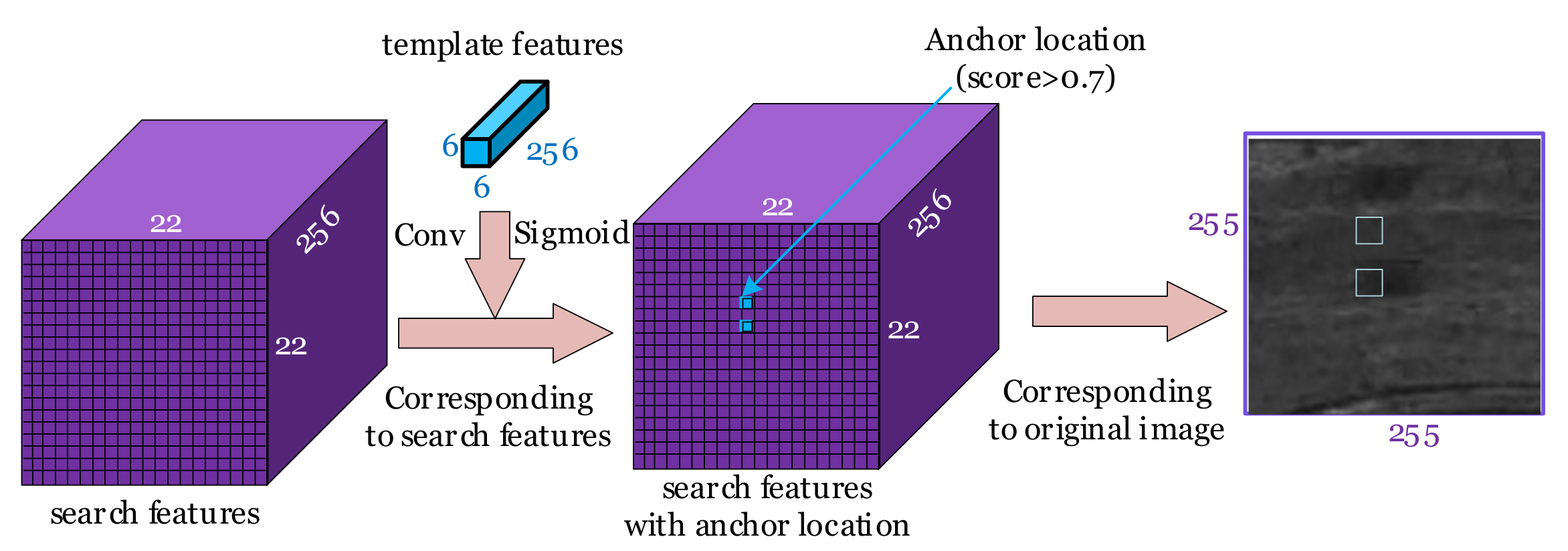
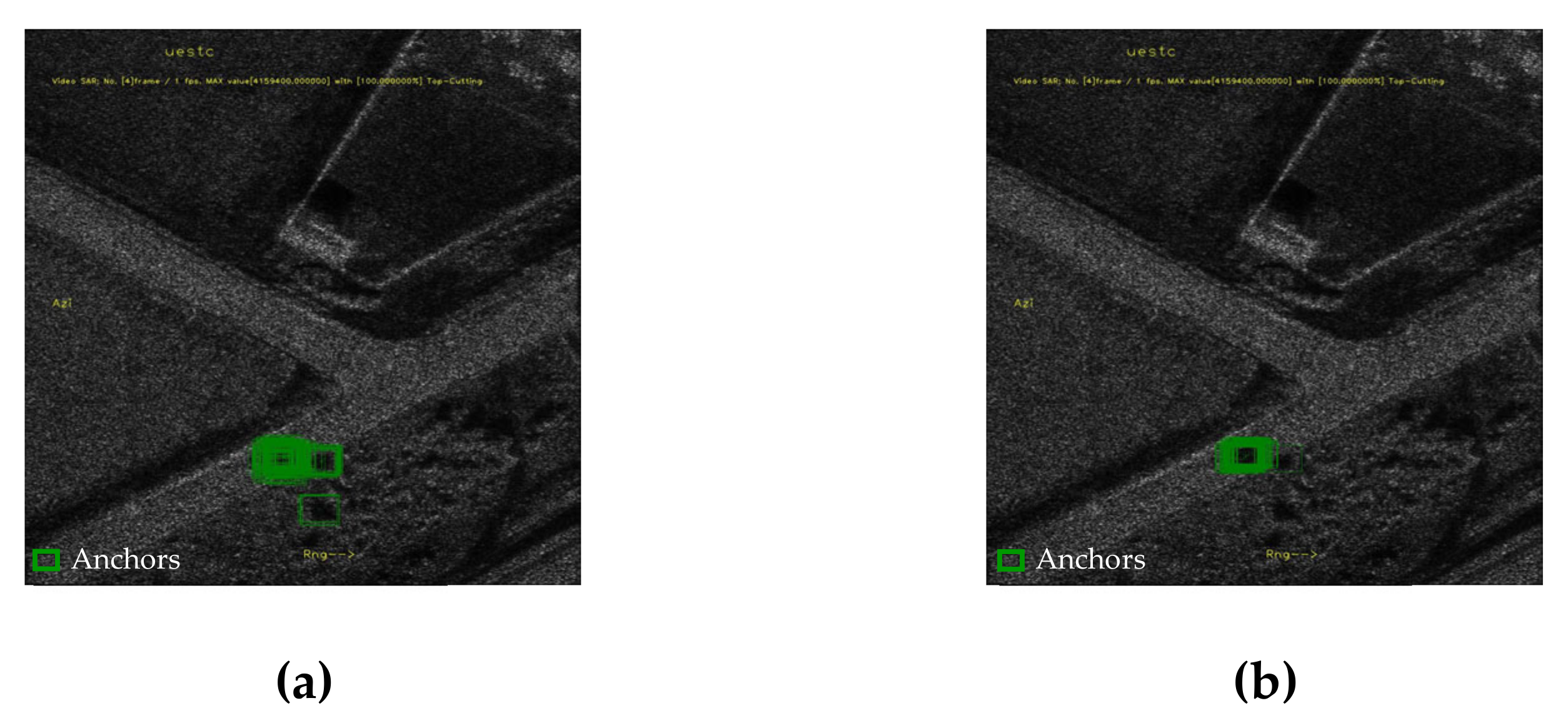
Step 4: Predict anchor location.
After obtaining the feature maps of the template and the search area, the predict anchor location module pre-determines the general location of the TOI in the search area to suppress false alarms. To only locate the anchors containing the center point of the shadow, the feature map of the template is used to convolute the feature map of the search area to obtain the prior information of the template, so that the score of each location of the output feature map represents the probability that the corresponding location is predicted to be the shadow. Then, the locations whose probability exceeds the preset threshold are used as the locations of the sparse anchors. As shown in
Figure 7, the blue regions correspond to the locations of the anchors.
Step 5: Predict anchor shape.
To generate the anchor that conforms to the shadow’s shape, the anchor shape prediction module generates an anchor shape with the highest coverage of the real shadow’s shape by adaptive prediction processing in the sparse locations. First, after anchor generation, the preset anchor shapes (marked with blue boxes in
Figure 8) of the anchor are obtained. Among them, the shape with the largest IoU with the shadow’s ground truth (marked with a green box) is predicted as the leading shape (marked with an orange box). After this, the leading shape of the anchor is regressed to obtain the best anchor shape (marked with a white box) that better conforms to the shadow’s shape.
Step 6: Adapt the feature map guided by anchors.
After the anchor shape prediction, the anchor shape changes, and the feature map needs to be adapted to guarantee the correct corresponding relationship between the feature map and the SAR images. As described in
Section 2.1.2, the adapted feature map can be generated by compensating the offset obtained from 1 × 1 convolution using the 3 × 3 deformable convolution. Based on the adapted feature map shown in
Figure 9 (marked with a dark purple), the higher quality anchors can be used for shadow tracking.
Step 7: Compare the similarity of the feature maps.
To compare the similarity of the feature map of the search area and the template, the similarity learning subnetwork applies the correlation operation as shown in
Figure 10a. The blue cube represents the feature map of the template, and the purple cube represents the feature map of the search area. The feature map of the template changes its channel by the convolution according to the number of anchors
k. The correlation can be achieved using the feature map of the template to convolute the feature map of the search area; then,
and
are output, where 2
k represents the probability of the foreground and background for each anchor, and 4
k represents the location (
x,
y) and shape (
w,
h) of the shadow.
Step 8: Classification and regression.
The similarity learning subnetwork is divided into classification and regression branches. In the classification branch, the similarity learning probability map of the foreground and background is obtained, and then the foreground anchor with the highest similarity learning metric is the tracking shadow. The regression branch further regresses the best anchor shape (marked with a white box) to achieve a more accurate shadow shape (marked with a red box) in
Figure 10b. Using the trained GASN, the shadow tracking in the Video-SAR image sequence can be achieved only using the shadow’s location and shape in the first frame.
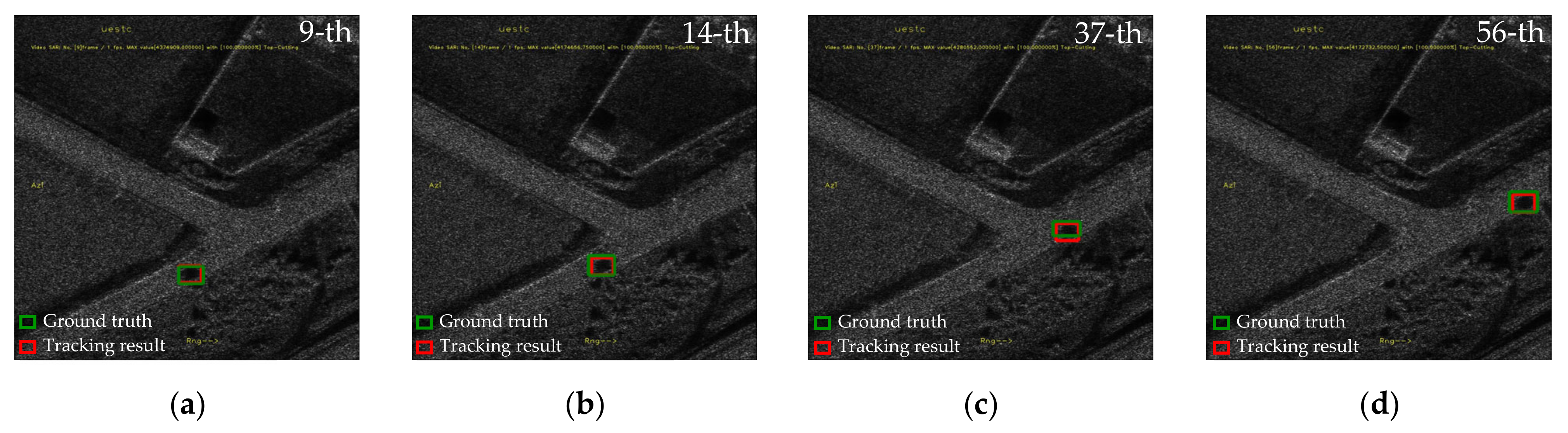
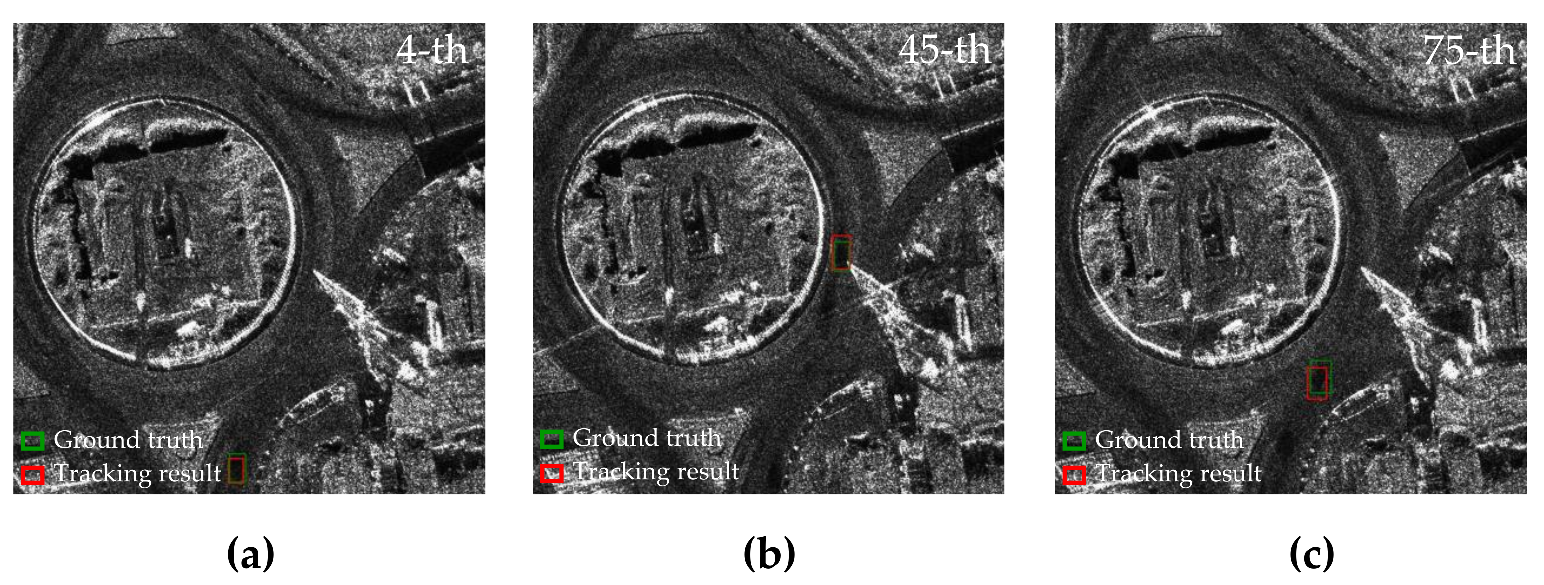
Step 9: Tracking results.
As shown in
Figure 10c, after searching the whole Video-SAR image sequence, the shadow, i.e., the TOI tracking of Video-SAR, is realized. Because the shadow’s location in the first frame is known, only the tracking results of the subsequent frames are shown here, where the green box represents the real location of the shadow, and the red box represents the tracking results.
To make the tracking process easier to read, it is shown in the Algorithm 1 below.
| Algorithm 1: GASN tracks arbitrary TOI in Video-SAR |
| Input: Video-SAR images sequence. |
| | Begin |
| 1 | do Pre-process the SAR images. |
| 2 |
|
| 3 | do Embed features by Siamese subnetwork. |
| 4 |
|
| 5 | do Predict anchor location. |
| 6 |
|
| 7 | do Predict anchor shape. |
| 8 |
|
| 9 | do Adapt the feature map guided by anchors. |
| 10 |
|
| 11 | do Compare the similarity of the feature maps. |
| 12 | |
| 13 | do Classification and regression. |
| 14 |
|
| | End |
| Output: Tracking results. |


