Article

A Novel Guided Anchor Siamese Network for Arbitrary Target-of-Interest Tracking in Video-SAR

School of Information and Communication Engineering, University of Electronic Science and Technology of China, Chengdu 611731, China
*
Author to whom correspondence should be addressed.
Remote Sens. 2021, 13(22), 4504; https://doi.org/10.3390/rs13224504
Submission received: 27 August 2021 / Revised: 28 October 2021 / Accepted: 1 November 2021 / Published: 9 November 2021
(This article belongs to the Special Issue Synthetic Aperture Radar (SAR) Meets Deep Learning)

Abstract

:
Video synthetic aperture radar (Video-SAR) allows continuous and intuitive observation and is widely used for radar moving target tracking. The shadow of a moving target has the characteristics of stable scattering and no location shift, making moving target tracking using shadows a hot topic. However, the existing techniques mainly rely on the appearance of targets, which is impractical and costly, especially for tracking targets of interest (TOIs) with high diversity and arbitrariness. Therefore, to solve this problem, we propose a novel guided anchor Siamese network (GASN) dedicated to arbitrary TOI tracking in Video-SAR. First, GASN searches for matching areas in the subsequent frames with the initial area of the TOI in the first frame are conducted, returning the most similar area using a matching function, which is learned from general training without TOI-related data. With the learned matching function, GASN can be used to track arbitrary TOIs. Moreover, we also constructed a guided anchor subnetwork, referred to as GA-SubNet, which employs the prior information of the first frame and generates sparse anchors of the same shape as the TOIs. The number of unnecessary anchors is therefore reduced to suppress false alarms. Our method was evaluated on simulated and real Video-SAR data. The experimental results demonstrated that GASN outperforms state-of-the-art methods, including two types of traditional tracking methods (MOSSE and KCF) and two types of modern deep learning techniques (Siamese-FC and Siamese-RPN). We also conducted an ablation experiment to demonstrate the effectiveness of GA-SubNet.

1. Introduction

Video synthetic aperture radar (Video-SAR) provides high-resolution SAR images at a faster frame rate, which is conducive to the continuous and intuitive observation of ground moving targets. Due to this advantage, Video-SAR brings about important applications in SAR moving target tracking [1]. Since the Sandia National Laboratory (SNL) of the United States first obtained high-resolution SAR images in 2003 [2], many scholars have investigated the problem of moving target tracking in Video-SAR [3,4,5,6,7]. However, due to different angles of illumination, the scattering characteristics of moving targets change with the movement of the platform. Worse still, it is difficult to track a moving target directly because the imaging results of the moving target usually shift from their true position.
Fortunately, shadow is caused by the ground being blocked by the moving target. Due to the absence of energy reflection, shadows appear at the real position of the moving target in the SAR image, with the advantage of a constant grayscale [8]. Therefore, shadow-aided moving target tracking has become a hot topic in Video-SAR. In recent years, many scholars have worked on shadow-aided moving target tracking in Video-SAR [9,10,11]. Wang et al. [9] fully considered the constant grayscale of shadows and used data multiplexing to achieve moving target tracking. Zhao et al. [10] applied the saliency-based detection mechanism and used spatial–temporal information to achieve moving target tracking in Video-SAR. Tian et al. [11] utilized the dynamic programming-based particle filter to achieve the track-before-detect algorithm in Video-SAR. However, the features used by these traditional methods are usually simple, which leads to the problem of the background being similar to the shadow, meaning it cannot be easily distinguished. Deep learning methods then emerged to solve shadow tracking due to their high accuracy and fast speed advantages [12,13,14,15,16]. Ding et al. [12] presented a framework for shadow-aided moving target detection using deep neural networks, which applied a faster region-based convolutional neural network (Faster-RCNN) [13] to detect shadows in a single frame and used a bi-directional long short-term memory (Bi-LSTM) [14] network to track the shadows. Zhou et al. [15] proposed a framework by combining a modified real-time recurrent regression network and a newly designed trajectory smoothing long short-term memory network to track shadows. Wen et al. [16] proposed a moving target tracking method based on the dual Faster-RCNN, which combined the shadow detection results in SAR images and the range-Doppler (RD) spectrum to suppress false alarms for moving target tracking in Video-SAR.
However, arbitrary target-of-interest (TOI) tracking is a challenge for the above methods. In this paper, we define TOI as a specific target in a video that one wants to track. TOI refers to the shadow to be tracked in Video-SAR. The reasons why arbitrary TOI tracking is a challenge are as follows: First, these methods are all based on appearance features, such as shape and texture. These methods need to train a large number of labeled training samples to extract appearance features, and the training samples must include the TOI. However, when we track an arbitrary TOI, it is impractical to collect samples of all categories for training because of the targets’ diversity and arbitrariness. Moreover, it takes extensive work and material resources to label a large number of SAR images. Therefore, these methods are both impractical and costly when tracking an arbitrary TOI in Video-SAR.
Thus, we propose a novel guided anchor Siamese network (GASN) for arbitrary TOI tracking in Video-SAR. First, the key of GASN lies in the idea of similarity learning, which learns a matching function to estimate the degree of similarity between two images. After training using a large number of paired images, the learned matching function in GASN, given an unseen pair of inputs (TOI in the first frame as the template, and the subsequent frame as the search image), is used to locate the area that best matches the template. As GASN only relies on the template information, which is independent of the training data, it is suitable for tracking arbitrary TOIs in Video-SAR. Additionally, a guided anchor subnetwork (GA-SubNet) in GASN is proposed to suppress false alarms and to improve the tracking accuracy. GA-SubNet uses the location information of the template to obtain the location probability in the search image, and then it selects the location with a probability greater than the threshold to generate sparse anchors, which can exclude false alarms. To improve the tracking accuracy, the anchor that more closely matches the shape of the TOI is obtained by GA-SubNet through adaptive prediction processing.
The main contributions of our method are as follows:
  • We established a new network GASN, which trains a large number of paired images to build a matching function to judge the degree of similarity between two inputs. After similarity learning, GASN matches the subsequent frame with the initial area of the TOI in the first frame and returns the most similar area as the tracking result.
  • We constructed a GA-SubNet embedded in GASN to suppress false alarms, as well as to improve the tracking accuracy. By incorporating the prior information of the template, our proposed GA-SubNet can generate sparse anchors that match the shape of the TOI the most.
To verify the validity of the proposed method, we performed experiments on simulated and real Video-SAR data. The results showed that the tracking accuracy of the proposed network is 60.16% on simulated Video-SAR data, 4.55% and 16.49% higher than the two deep learning methods Siamese-RPN [17] and Siamese-FC [18], as well as 18.36% and 28.95% higher than the two traditional methods MOSSE [19] and KCF [20], respectively. Meanwhile, the tracking accuracy is 54.68% on real Video-SAR data, which is higher than the other four methods by 1.93%, 13.08%, 14.70%, and 25.04%, respectively. This demonstrates that our method can achieve accurate arbitrary TOI tracking in Video-SAR.
The rest of this paper is organized as follows: Section 2 introduces the methodology, including the network architecture, preprocessing, and tracking processes. Section 3 introduces the experiments, including the simulated and real data, the implementation details, the loss function, and the evaluation indicators. Section 4 introduces the simulated and real Video-SAR data tracking results. Section 5 discusses the research on pre-training and robustness and the ablation experiment. Section 6 provides the conclusion.

2. Methodology

2.1. Network Architecture

Figure 1 shows the architecture of GASN for arbitrary TOI tracking in Video-SAR, including the Siamese subnetwork, GA-SubNet, and the similarity learning subnetwork. GASN is based on the idea of similarity learning, which compares a template image z to a search image x and returns a high score if the two images depict the same target.
To prepare for similarity learning, the Siamese subnetwork consists of a template branch and a search branch. The two branches apply identical transformation φ to each input, and the transformation φ can be considered as feature embedding. Then, similarity learning can be expressed as f (z, x) = g (φ(z), φ(x)), where the function g is a similarity metric. To suppress false alarms, GA-SubNet receives the prior information from the template to pre-determine the general location and shape of the TOI in the search image using anchors. When tracking an arbitrary TOI that is different from the training sample, we can use the ability of similarity learning to find the TOI in the next frame by providing the template information of said TOI, such as the position and shape. The similarity learning subnetwork is divided into two branches, one for the classification of the shadow and background, and the other for the regression of the shadow’s location and shape. In both branches, the similarity between the shadow template and the search area is calculated, and then the target with the maximum similarity to the template of the TOI is chosen as the tracking result.
GASN always uses the previous frame as the template image and the current frame as the search image. After testing the whole SAR image sequence in such a way, GASN can achieve arbitrary TOI tracking in Video-SAR. In the following, we introduce the three subnetworks of GASN in detail in the order of implementation.

2.1.1. Siamese Subnetwork

The Siamese subnetwork (marked as the green region in Figure 1) [21,22] uses CNN for feature embedding. CNN uses different convolutional kernels for multi-level feature embedding of the image. Therefore, compared to the traditional manual features, the features embedded by the Siamese subnetwork are more representative and can describe the TOI better. To obtain the common features of the previous and current frames, the Siamese subnetwork is divided into a template branch (marked with a purple box) and a search branch (marked with a pink box), and the parameters of CNN-1 and CNN-2 in both branches are shared to ensure the consistency of features. The input of the template branch is the TOI area in the previous frame (denoted as z), and the input of the search branch is the search area in the current frame (denoted as x). See Section 2.2 for details about the preprocessing of the input images. For convenience, we denote the output feature maps of the template and search branches as φ(z) and φ(x).

2.1.2. GA-SubNet

After obtaining the feature maps, we established a GA-SubNet to suppress false alarms and improve the tracking accuracy. The specific architecture of GA-SubNet is shown in Figure 2, including anchor location prediction, anchor shape prediction, and feature adaptation. In the following, we introduce the three modules of GA-SubNet in detail in the order of implementation.
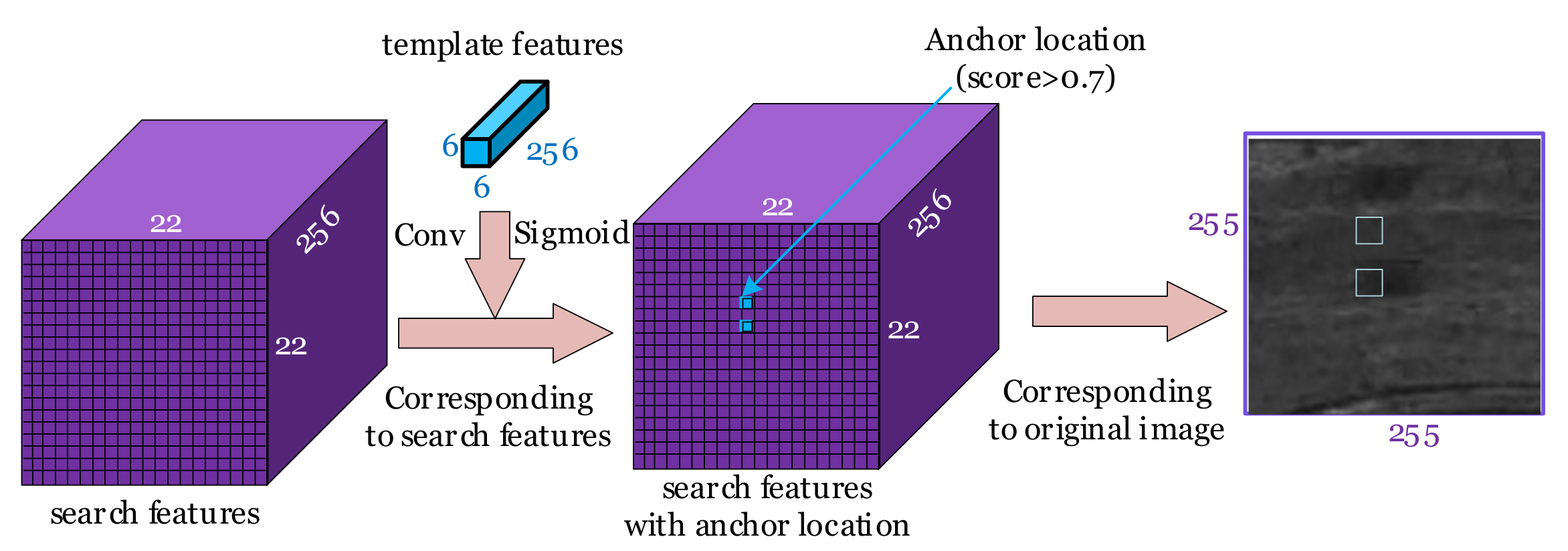
The purple region in Figure 2a is the anchor location prediction, i.e., the prediction of the location of the anchor containing the center point of a shadow. First, the input to GA-SubNet is two feature maps, one for the template (marked with a blue cube) and the other for the search area (marked with a purple cube). To obtain the prior information of the template that is independent of the training data, the feature map of the template is used as the kernel to convolute the feature map of search area F1, so that the score of each location of the output represents the probability that the corresponding location is predicted to be the shadow. Then, the sigmoid function is used to obtain the probability map as shown in the blue box in Figure 2a. After this, the position whose probability exceeds the preset threshold is chosen to be the location of the predicted anchor (marked with a red circle). To learn more information about the shadow, similar to [17], the empirical threshold was chosen as 0.7.
The blue region in Figure 2b is the anchor shape prediction, i.e., the prediction of the anchor shape that better conforms to the shape of a shadow. First, the uniform arbitrary preset anchor shapes are generated (marked with blue boxes) at each location obtained from the anchor location prediction; i.e., several anchor shapes are arbitrarily set at each location, but the anchor shape setting in sparse locations is uniform. The preset anchor shape with the largest IoU with the shadow’s ground truth (marked with a green box) is predicted as the leading shape (marked with an orange box). IoU is defined by Equation (1), where P denotes the preset anchor shapes, and G denotes the shadow’s ground truth.
IoU = area ( P G ) area ( P G )
The leading shape of the anchor is still set arbitrarily and may differ significantly from the shadow’s ground truth. To make the IoU larger, the offset between the leading shape and the shadow’s ground truth at each location is calculated. After continuously optimizing the offsets using the loss function (described in Section 3.3), the best anchor shape can be obtained (marked with a white box), which better conforms to the shape of the shadow.
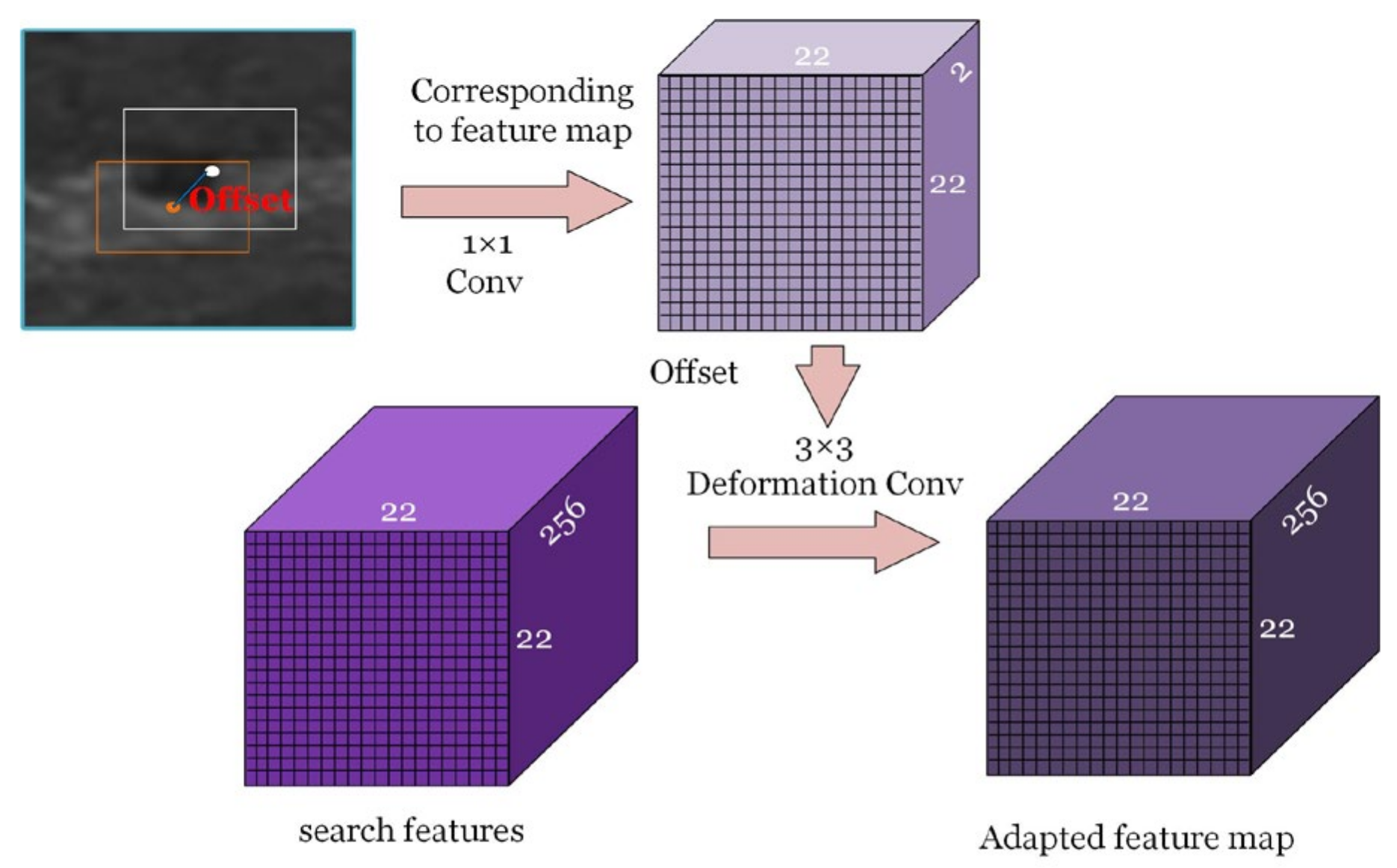
The orange region in Figure 2c is the feature adaptation, i.e., the adaptation of the feature map and the SAR image. Because the feature map is obtained by multi-layer convolution of the SAR image, there is a certain correspondence between the feature map and the SAR image; i.e., the leading shape of the anchor in the SAR image corresponds to a specific region in the feature map. However, the leading shape of the anchor at each location is optimized adaptively in the anchor shape prediction, resulting in areas with the same shape in the feature map, corresponding to the areas with different shapes in the SAR image. Therefore, feature adaptation is necessary to satisfy the correspondence between the feature map and the SAR image to ensure the accuracy of tracking. First, 1 × 1 convolution is used to calculate the offset between the leading shape and the best shape. Then, 3 × 3 deformed convolution is applied [23,24] based on this offset to the original feature map F1 of the search area. Finally, the feature map F2 is obtained for adaptation to the SAR image for the best anchor shape.

2.1.3. Similarity Learning Subnetwork

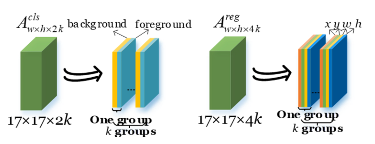
After obtaining the sparse anchors that better conform to the shadows’ shape, the similarity learning subnetwork (marked with a yellow region in Figure 1) is used for classification and regression. The similarity learning subnetwork consists of a classification branch (marked with an orange box in Figure 1) for distinguishing the shadow from the background and a regression branch (marked with a blue box in Figure 1) for predicting the location and shape of the shadow. First, in both branches, to reduce the calculation complexity for subsequent similarity learning, a feature map 6 × 6 of φ(z) is reduced to 4 × 4 and a feature map 22 × 22 of φ(x) is reduced to 20 × 20 by using the convolutions (marked with yellow cubes in Figure 1). In addition, the channel of φ(z) is adjusted to 2k × 256 for the foreground and background classification in the classification branch. The channel of φ(z) is adjusted to 4k × 256 for determining the location and shape of the shadow in the regression branch. k is the number of anchors, 2k represents the probability of the foreground and background for each anchor, and 4k represents the location (x, y) and shape (w, h) of the shadow.
A w × h × 2 k c l s = [ φ ( x ) ] cls [ φ ( z ) ] cls A w × h × 4 k r e g = [ φ ( x ) ] reg [ φ ( z ) ] reg
As shown in Equation (2), the similarity learning subnetwork applies pairwise correlations (marked with red rectangles in Figure 1) to calculate the similarity metric, in which the similarity map A w × h × 2 k cls is for classification and A w × h × 4 k reg is for regression. [ · ] cls and [ · ] reg represent the classification and regression, respectively, and denotes the convolution operation. We show the feature composition of A w × h × 2 k cls and A w × h × 4 k reg in Figure 3. A w × h × 2 k cls is divided into k groups, and each group contains two feature maps, which indicate the foreground and background probabilities of the corresponding anchors. The anchor is the foreground if the probability of the foreground is higher; otherwise, it is the background. Similarly, A w × h × 4 k reg is divided into k groups, and each group contains four feature maps (x, y, w, and h), which indicate the similarity metric between the corresponding anchor and the template. According to the highest similarity, the optimal location and the shape of the shadow are obtained.

2.2. Preprocessing

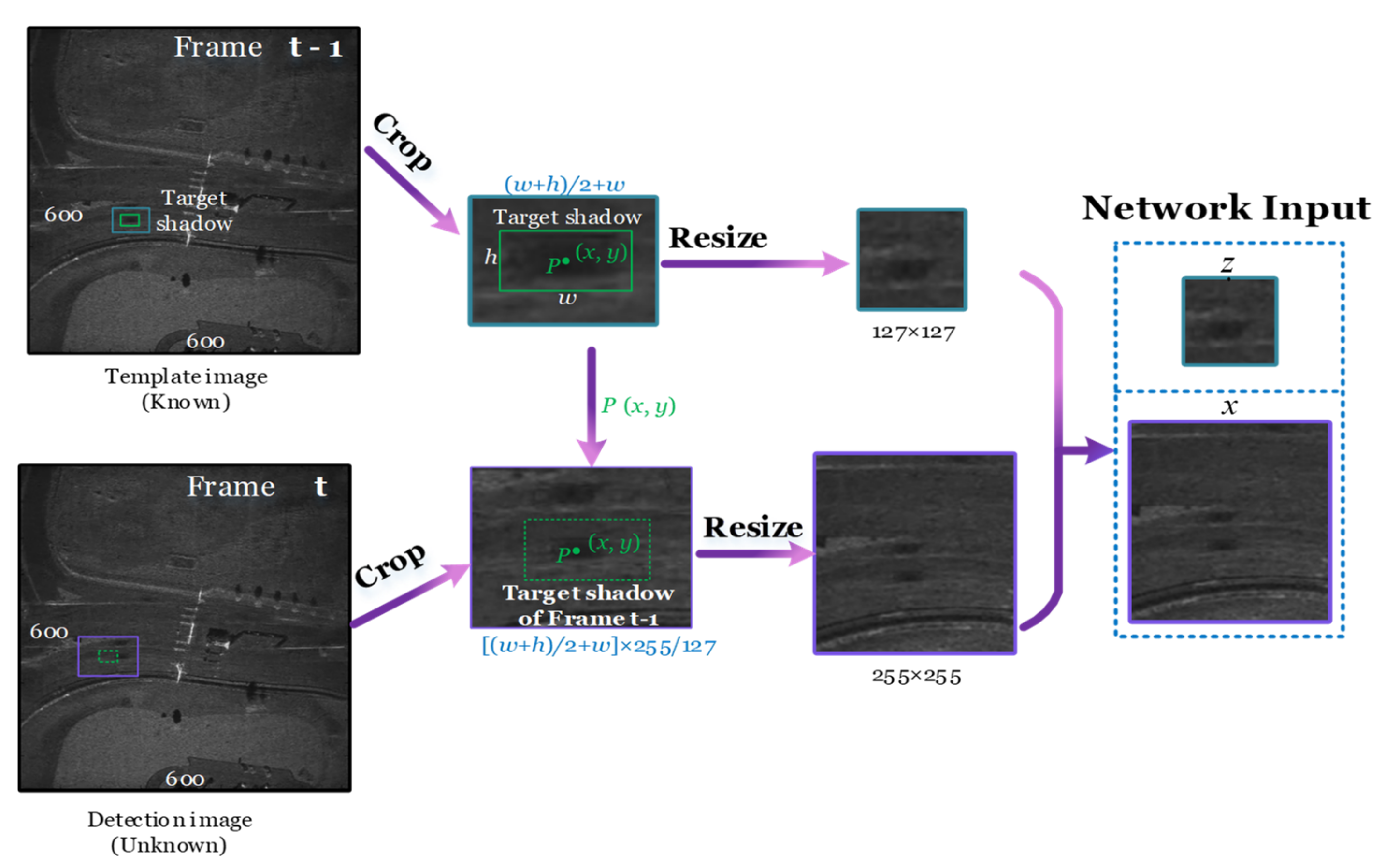
For all images of Video-SAR to have the same feature dimensions, preprocessing is required before entering GASN. As shown in Figure 4, the input of GASN is a pair of adjacent images in the SAR image sequence. The shadow template is a 127 × 127 area centered on the center (x, y) of the shadow in frame t-1. Similar to the image preprocessing in [17], we cropped an ((w + h) × 0.5 + w, (w + h) × 0.5 + h) area in frame t-1 centered on (x, y) and then resized it to 127 × 127, where (w, h) is the boundary of the shadow. Here, (x, y, w, and h) are known in the training stage, while in the testing stage, the parameters represent the prediction results of the previous frame. Because the template size of all existing methods is 127 × 127 [17,18], to ensure the rationality of the comparison, we chose 127 × 127 as the template size. The search area is centered on the center of the shadow in frame t, and we cropped an (((w + h) × 0.5 + w) × 255/127, ((w + h) × 0.5) + h) × 255/127) area and then resized it to 255 × 255. This area is larger than the shadow’s template to ensure that the shadow is always included in the search area.

2.3. Tracking Process

The whole process of TOI tracking based on GASN is shown in Figure 5. The details are as follows.
Step 1: Input Video-SAR image sequence.
As shown in Figure 6a, N is the number of frames of the input video. For easy observation, we marked the shadow to be tracked with a green box.
Step 2: Preprocessing SAR images.
For all images of Video-SAR to have the same feature dimensions, we need to crop and resize them. As described in Section 2.2, the shadow in frame t-1 is resized to 127 × 127 as the template, and frame t is resized to 255 × 255 as the search area, as shown in Figure 6b. x, y, w, and h represent the center and boundary of the prediction results in the previous frame. Unlike the RGB three-channel optical images, the SAR images are gray; therefore, all three channels are assigned to the same gray value to use the pre-trained weights. Applying models trained on three-channel RGB images to one-channel radar images has been carried out in several published literatures [10,12,15], and the results in Section 5.3 show that it is reasonable to do so.
Step 3: Embed features by the Siamese subnetwork.
After obtaining the template and search areas, the Siamese subnetwork embeds features to better describe the TOI. The Siamese subnetwork is divided into a template branch and a search branch, and the parameters of CNN-1 and CNN-2 in the two branches are shared to ensure the consistency of the features. The template branch outputs 6 × 6 × 256 as the feature map of the template, and the search branch outputs 22 × 22 × 256 as the feature map of the search area, which are shown in Figure 6c.
Step 4: Predict anchor location.
After obtaining the feature maps of the template and the search area, the predict anchor location module pre-determines the general location of the TOI in the search area to suppress false alarms. To only locate the anchors containing the center point of the shadow, the feature map of the template is used to convolute the feature map of the search area to obtain the prior information of the template, so that the score of each location of the output feature map represents the probability that the corresponding location is predicted to be the shadow. Then, the locations whose probability exceeds the preset threshold are used as the locations of the sparse anchors. As shown in Figure 7, the blue regions correspond to the locations of the anchors.
Step 5: Predict anchor shape.
To generate the anchor that conforms to the shadow’s shape, the anchor shape prediction module generates an anchor shape with the highest coverage of the real shadow’s shape by adaptive prediction processing in the sparse locations. First, after anchor generation, the preset anchor shapes (marked with blue boxes in Figure 8) of the anchor are obtained. Among them, the shape with the largest IoU with the shadow’s ground truth (marked with a green box) is predicted as the leading shape (marked with an orange box). After this, the leading shape of the anchor is regressed to obtain the best anchor shape (marked with a white box) that better conforms to the shadow’s shape.
Step 6: Adapt the feature map guided by anchors.
After the anchor shape prediction, the anchor shape changes, and the feature map needs to be adapted to guarantee the correct corresponding relationship between the feature map and the SAR images. As described in Section 2.1.2, the adapted feature map can be generated by compensating the offset obtained from 1 × 1 convolution using the 3 × 3 deformable convolution. Based on the adapted feature map shown in Figure 9 (marked with a dark purple), the higher quality anchors can be used for shadow tracking.
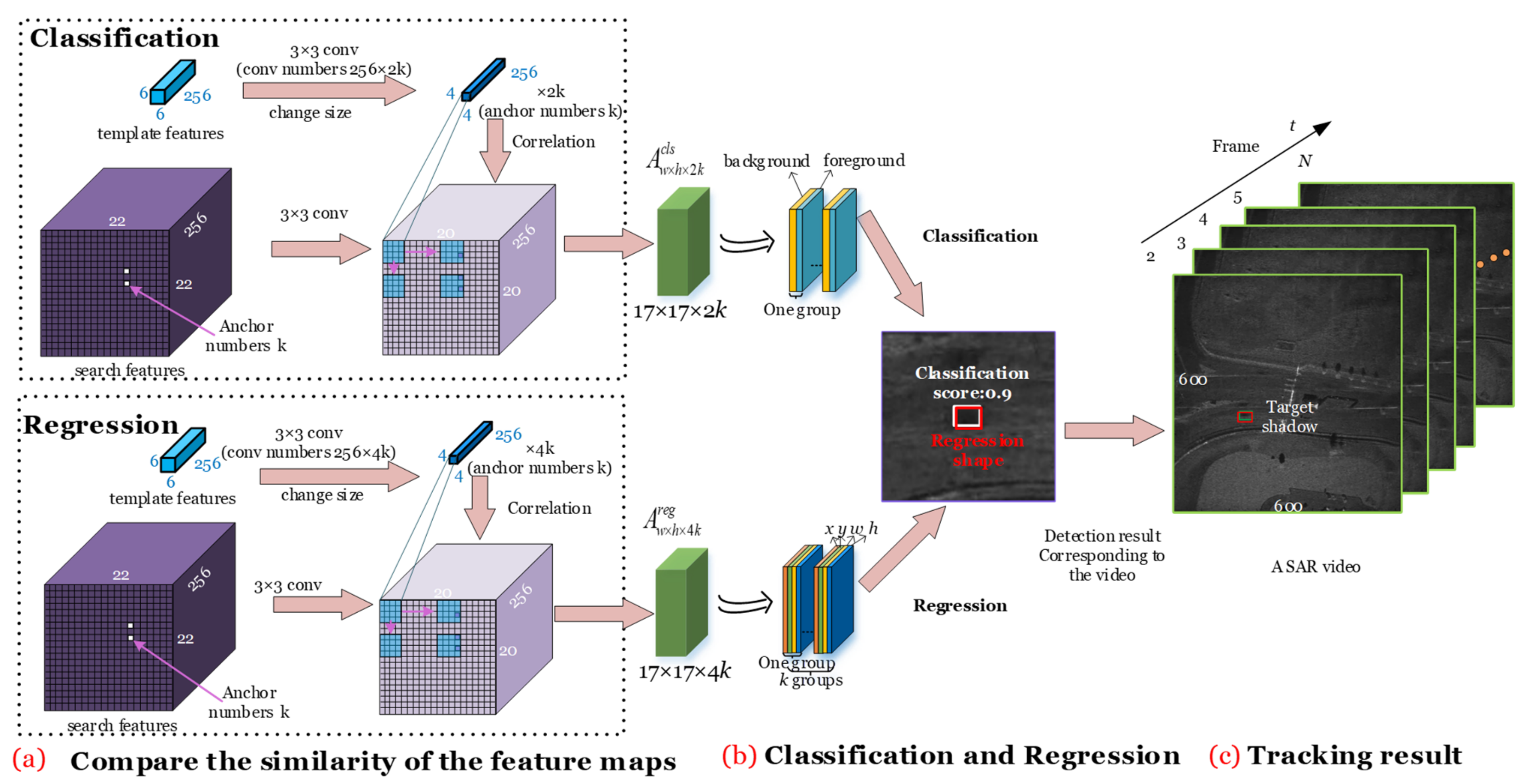
Step 7: Compare the similarity of the feature maps.
To compare the similarity of the feature map of the search area and the template, the similarity learning subnetwork applies the correlation operation as shown in Figure 10a. The blue cube represents the feature map of the template, and the purple cube represents the feature map of the search area. The feature map of the template changes its channel by the convolution according to the number of anchors k. The correlation can be achieved using the feature map of the template to convolute the feature map of the search area; then, A w × h × 2 k cls and A w × h × 4 k reg are output, where 2k represents the probability of the foreground and background for each anchor, and 4k represents the location (x, y) and shape (w, h) of the shadow.
Step 8: Classification and regression.
The similarity learning subnetwork is divided into classification and regression branches. In the classification branch, the similarity learning probability map of the foreground and background is obtained, and then the foreground anchor with the highest similarity learning metric is the tracking shadow. The regression branch further regresses the best anchor shape (marked with a white box) to achieve a more accurate shadow shape (marked with a red box) in Figure 10b. Using the trained GASN, the shadow tracking in the Video-SAR image sequence can be achieved only using the shadow’s location and shape in the first frame.
Step 9: Tracking results.
As shown in Figure 10c, after searching the whole Video-SAR image sequence, the shadow, i.e., the TOI tracking of Video-SAR, is realized. Because the shadow’s location in the first frame is known, only the tracking results of the subsequent frames are shown here, where the green box represents the real location of the shadow, and the red box represents the tracking results.
To make the tracking process easier to read, it is shown in the Algorithm 1 below.
Algorithm 1: GASN tracks arbitrary TOI in Video-SAR
Input: Video-SAR images sequence.
Begin
1do Pre-process the SAR images.
2 127 × 127 × 3 template   image ,   255 × 255 × 3 search   image
3do Embed features by Siamese subnetwork.
4 6 × 6 × 256 127 × 127 × 3 CNN - 1 , 22 × 22 × 256 255 × 255 × 3 CNN - 2
5do Predict anchor location.
6 score F 1 1 × 1 conv ,   probability map score sigmoid location probability map > 0 . 7
7do Predict anchor shape.
8 IoU = area ( P G ) area ( P G ) , shape max ( IoU )
9do Adapt the feature map guided by anchors.
10 offset F 1 1 × 1 conv , F 2 F 1 3 × 3 deformabel conv based   on   offset
11do Compare the similarity of the feature maps.
12 4 × 4 × 256 × 2 k 6 × 6 × 256 , 4 × 4 × 256 × 4 k 6 × 6 × 256 , 20 × 20 × 256 22 × 22 × 256 17 × 17 × 2 k 4 × 4 × 256 × 2 k 20 × 20 × 256 17 × 17 × 4 k 4 × 4 × 256 × 4 k 20 × 20 × 256
13do Classification and regression.
14 Classification max ( 17 × 17 × 2 k ) , Regression max ( 17 × 17 × 4 k )
End
Output: Tracking results.

3. Experiments

All of the experiments were implemented on a personal computer with an Intel Core i7-8700K [email protected] and an NVIDIA GTX1080 graphics card with 8 GB of memory. The software experiment environment was Linux, Ubuntu 16.04, python 3.7, and Pytorch3.0.

3.1. Experimental Data

As existing recognized real Video-SAR data, due to the high resolution, the data of SNL [1] have been used by many scholars for moving target detection and tracking [7,8,9,10]. In our experiments, we used both the simulated and real data to verify the effectiveness of GASN for arbitrary TOI tracking in Video-SAR. We produced the simulated Video-SAR data from the echo to approximate real SAR images, and the details of the data are described below.
In the simulated Video-SAR data, two real SAR backgrounds containing roads and six moving targets were simulated, considering the generality. The radar system parameters and the velocity of the moving targets are listed in Table 1 and Table 2. Regarding the simulation of the shadow, the scattering coefficient was set to zero because of no reflection. In the experiment, 17 videos were simulated, where 11 videos were utilized for training and 6 for testing. Each video contained 61 frames, and one of the test video sequences is shown in Figure 11. The size of all images was 600 × 600.
The real Video-SAR SNL data contained 50 different moving targets in all 899 frames. When GASN was used for arbitrary TOI tracking, 751 frames with the former 35 targets were set for training, and 148 frames with the latter 15 targets were set for testing. The size of all images was 600 × 600. Compared to the simulated data, there was more noise and clutter in the real Video-SAR data, and the tracking results with clutter are shown in Section 4.2.2.

3.2. Implementation Details

To avoid over-fitting, the pre-trained weight of ResNet50 [25] was applied, which was successfully trained from the widely used ImageNet large-scale visual recognition challenge (ILSVRC) data set [26]. Unlike the three-channel RGB for optical images, the SAR images were all gray; therefore, we assigned all three channels to the same gray value to use the pre-trained weights. Due to the limited memory, only conv4 and the upper layers of the pre-trained network weights were fine-tuned for adaptation to the TOI tracking task in Video-SAR. During the training stage, the batch size was four, and the stochastic gradient descent (SGD) [27] was applied, in which the momentum was 0.9, the weight decay was 0.0005, and the learning rate was 0.0001.
Data augmentation techniques were used in our implementation, including translation, scale transformations, blur, and flip. After data augmentation, the amount of data expanded by approximately 10 times, which can better fine-tune the model.

3.3. Loss Function

As shadow occupies a small proportion of the SAR image, we used focal loss [28] as the anchor location loss loss loc to predict the anchor location:
loss loc = ( 1 p ) γ log ( p )
where p is the probability of the shadow in the location, and γ = 2 is the hyper-parameter to adjust the drop speed influenced by [29].
Anchor shape loss loss shape uses a smooth L1 loss inspired by [12].
l o s s s h a p e s = s m o o t h L 1 ( 1 min ( w w g , w g w ) ) + s m o o t h L 1 ( 1 min ( h h g , h g h ) )
s m o o t h L 1 = 0.5 x x < 1 x - 0.5 o t h e r w i s e
where ( w g , h g ) is the ground truth of the shadow, and ( w , h ) is the shape of the anchor.
As per Siamese-RPN [17], classification loss loss cls and regression loss loss reg are as follows:
loss cls = log [ p i * p i + ( 1 p i * ) ( 1 p i ) ]
loss reg = s m o o t h L 1 ( t i t i * )
where p i represents the probability of shadow, t represents the ground truth of the center point (x, y) and shape (w, h) of the shadow, and * represents the prediction result.
The total loss function is shown below, where λ 1 = λ 2 = 5 and λ 3 = λ 4 = 2 are the hyper-parameters balancing the four parts.
loss = λ 1 loss loc + λ 2 loss shape + λ 3 loss cls + λ 4 loss reg
By minimizing the loss functions, GASN finally achieves parameter optimization after the iterations.

3.4. Evaluation indicators

To verify the performance of GASN, three general evaluation indicators were used in this paper.

3.4.1. Tracking Accuracy

The expected average overlap (EAO) can represent the tracking accuracy [30], and the greater the EAO, the more accurate the tracking result. EAO is defined as follows:
EAO = j = 1 N s mIoU (   j ) N s , mIoU = i = 1 N IoU ( P i , G ) N
where IoU is as defined in Equation (1), P is the tracking result, G is the shadow’s ground truth, N is the number of images in the Video-SAR sequence, and Ns is the number of videos in the test data. We calculated mIoU, including IoU = 0; therefore, EAO can truly reflect the tracking accuracy.

3.4.2. Tracking Stability

The central location error (CLE) reflects the stability of the tracking method [15]; i.e., the smaller the CLE, the more stable the tracking method, and the CLE is defined as follows:
C L E = ( x R - x G ) 2 + ( y R - y G ) 2
where ( x R , y R ) represents the central location of the tracking result, and ( x G , y G ) represents the central location of the shadow’s ground truth.

3.4.3. Tracking Speed

The frames per second (FPS) represent the tracking speed, which is defined as follows:
F P S = N t
where t represents the total tracking time, and N is the number of images in the Video-SAR sequence.

4. Results

4.1. Results of the Simulated Video-SAR Data

Figure 12 shows the tracking results of the simulated Video-SAR data. In the rest of this paper, the red box represents the tracking results, and the green box represents the ground truths of the shadow. It can be seen that the red and green boxes have a great overlap, which means that GASN can track the target effectively.
We quantitatively analyzed the tracking results of GASN. Because Siamese-FC and Siamese-RPN significantly outperform MOSSE [19] and KCF [20], only the visual comparison results of GASN with Siamese-RPN and Siamese-FC in terms of accuracy, CLE, and FPS indicators are shown.

4.1.1. Comparison with Other Tracking Methods

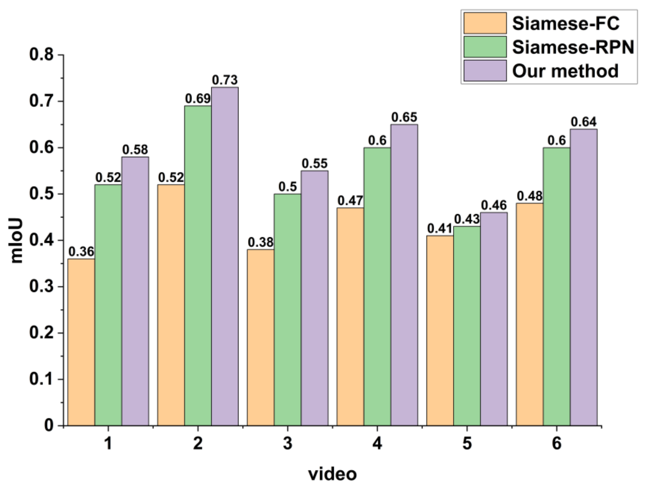
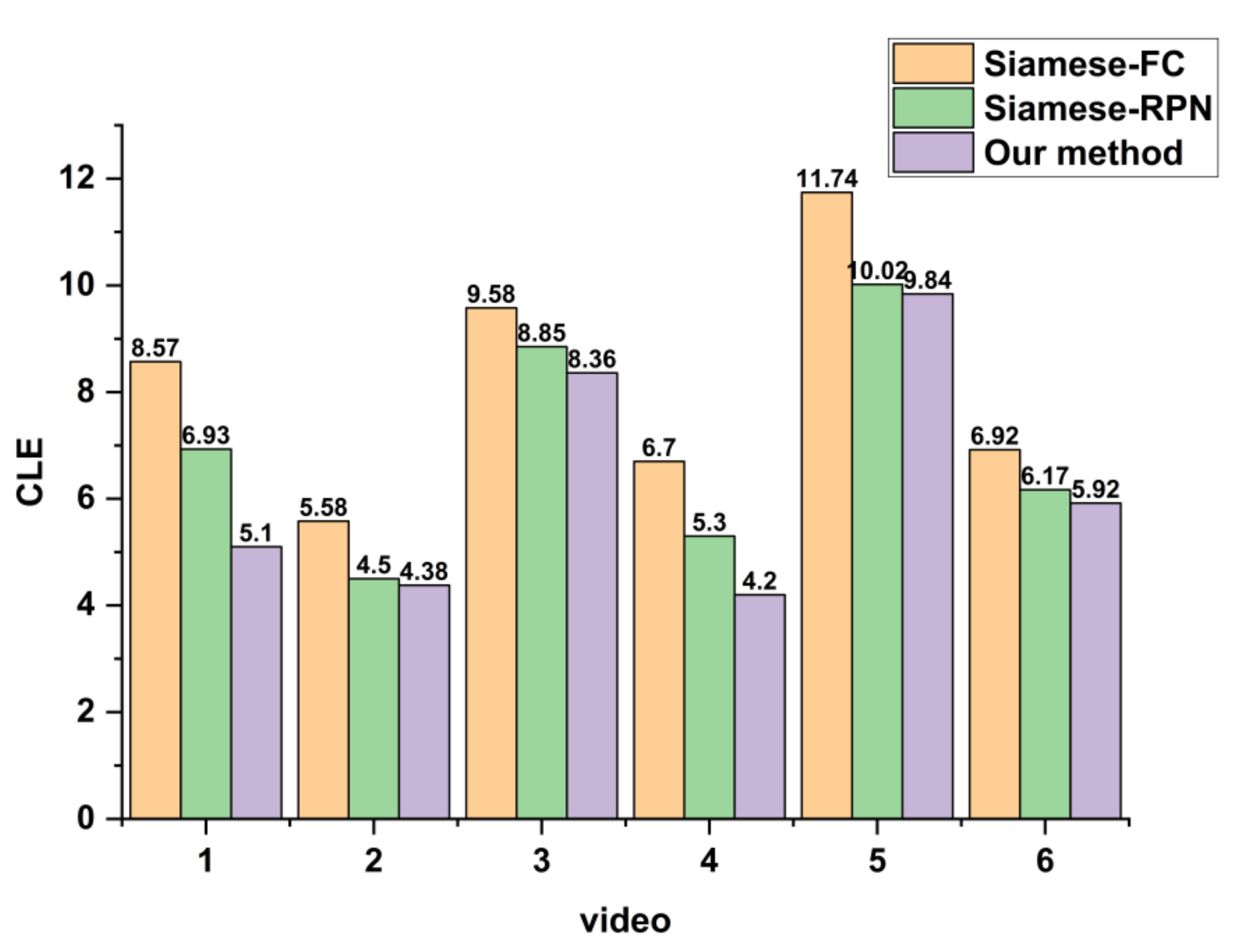
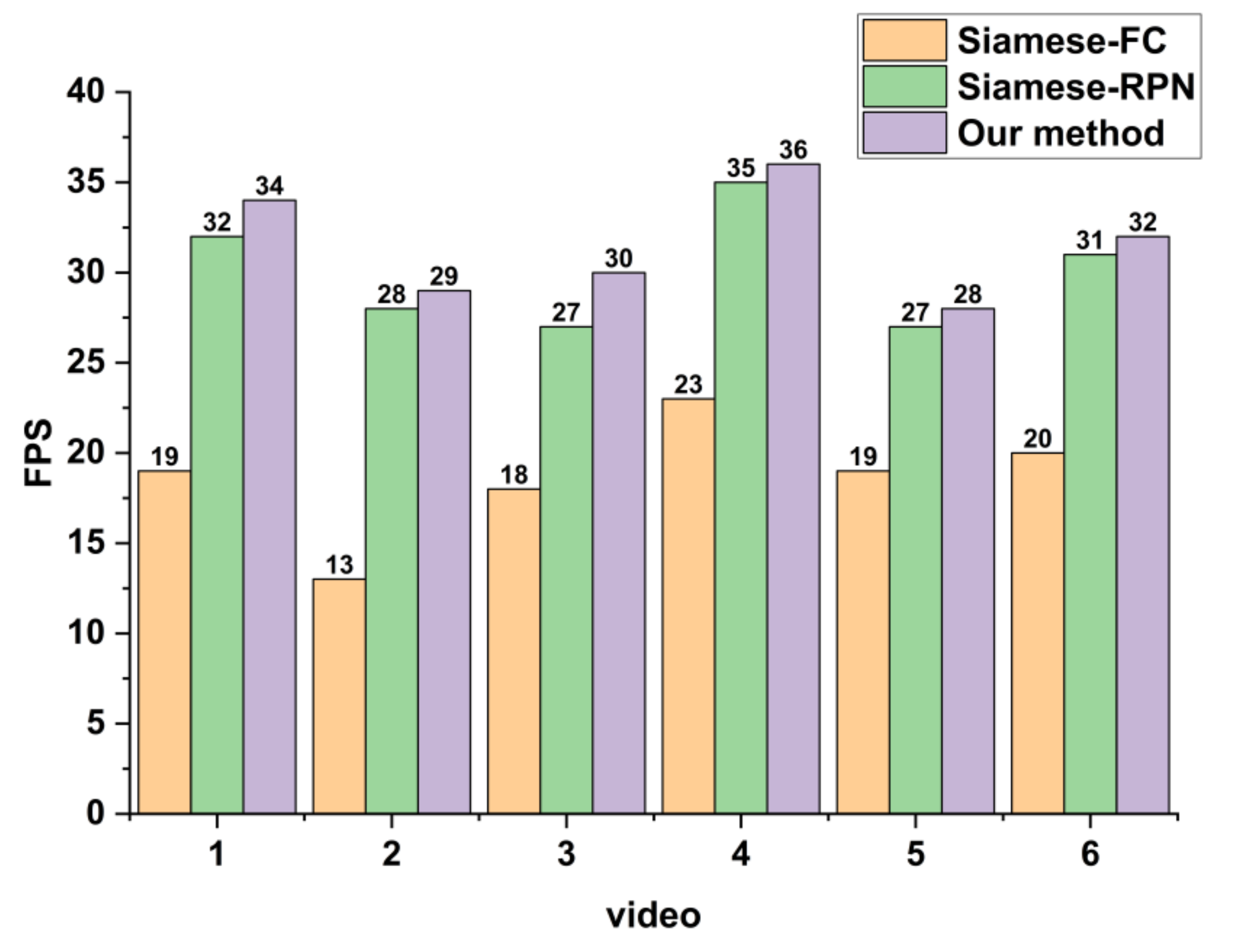
Figure 13, Figure 14, and Figure 15 show the results of comparing GASN to Siamese-RPN and Siamese-FC on the six test videos. In the comparative experiments, we retrained Siamese-FC and Siamese-RPN using the same simulated data, and both networks were tuned. Moreover, to ensure the rationality of the experiments, our comparative experiments were all performed under the same conditions, such as the data preprocessing, the hard and soft platforms, and the training mechanism. From the results, we can see that GASN (marked with purple) obtained the highest mIoU (Figure 13) and the lowest CLE (Figure 14) on each video. Moreover, the FPS (Figure 15) of GASN (marked with purple) was almost the same as that of Siamese-RPN (marked with green), which indicates that GASN has almost no speed loss at a higher accuracy. Due to the above phenomenon also applying to real data, we explain the reason in detail in the next section. To reveal the performance of GASN more intuitively, we calculated the average tracking performance of the six testing videos, and the results are shown in Table 3.
In Table 3, for the two traditional methods (MOSSE and KCF), their simple framework leads to two different implications. On the one hand, these methods require low computation (105 FPS for MOSSE and 58 FPS); on the other hand, the simple framework may cause the loss of some information, such as the edges and textures, resulting in the inability to track shadows that are too wide or too long, and, therefore, the accuracy is low (31.21% for MOSSE and 41.80% for KCF). As for the comparison between deep learning methods, the anchors generated by GA-SubNet can better conform to the shape of the shadow in SAR images. Therefore, the accuracy of GASN (60.16%) is better than that of Siamese-RPN (55.61%) or Siamese-FC (43.67%). As for the tracking speed, GASN also slightly improved (32 FPS) compared to Siamese-RPN (31 FPS), because the anchors generated by GA-SubNet are sparse. In addition, GASN achieved the lowest CLE score (6.68) when considering the stability, because GA-SubNet generates anchors based on the probability of the shadow’s location. Through the above analysis, we can see that the tracking performance of GASN is better than that of the other methods.

4.1.2. Tracking Results with Distractors

To verify that the proposed method only tracks the TOI, we selected two adjacent targets with similar shapes for tracking. Figure 16a,b show the tracking results in the same frame. TOI-2 can be considered a distractor when we want to track TOI-1 in Figure 16a. Similarly, TOI-1 can be considered a distractor when we want to track TOI-2 in Figure 16b. The green box represents the ground truth of the TOI, and the red box represents the tracking results using the proposed method. The overlap between the red and green boxes in both figures is greater than 50%, so the proposed method can accurately track the TOI without errors. The main reasons are as follows: GASN uses the Siamese subnetwork to extract multi-level and more expressive features compared to the traditional methods. In addition, compared to the existing deep learning methods, GASN uses GA-SubNet to provide the general location and shape of the TOI based on the template, which can effectively suppress the distractors. Through the above analysis, we think that the proposed method can accurately track the TOI without errors, although there are distractors in the scene.

4.1.3. Tracking Results of the Target with a Specific Speed

To verify the tracking capability of the proposed method for TOI with a specific speed, we simulated two identical targets, except for the velocity. Figure 17a,b show the tracking results in the same frame. The azimuth velocity of TOI-1 in Figure 17a is 2 m/s and the radial velocity is –2.5m/s, while the azimuth velocity of TOI-2 in Figure 17b is 1.5 m/s and the radial velocity is –1.5m/s. The green box represents the ground truth of the TOI in this tracking process, and the red box represents the tracking result using the proposed method. The overlap between the red and green boxes in both figures is greater than 50%. Therefore, it can be seen that the proposed method can accurately track the TOI with a specific speed.

4.2. Results of Real Video-SAR Data

Figure 18 shows the tracking results using the real Video-SAR data, aiming to verify the effectiveness of GASN using real data. It can be seen that the tracking results (marked with a red box) and the ground truths of the shadow (marked with a green box) have a great overlap (the IoU is greater than 50%), which means that GASN can track the real shadow effectively.

4.2.1. Comparison with Other Tracking Methods

In the comparative experiments, with the same training mechanism as GASN, we first initialized Siamese-FC and Siamese-RPN using the pre-trained model parameters obtained from the optical image. Then, we adjusted the model parameters using SAR images for tracking in Video-SAR. Moreover, to ensure the rationality of the experiments, our comparative experiments were all performed under the same conditions, such as the data preprocessing and the hard and soft platforms.
Figure 19 shows the accuracy comparison results of the three methods. Siamese-FC (marked with yellow) had the lowest accuracy in each video because it cannot fit the scale transformation of the shadow. For Siamese-RPN (marked with green), the accuracy improved somewhat, because the anchors can handle scale transformation. However, most preset anchors do not perfectly fit the actual shape of the shadow, which results in failure when tracking shadows that are too long or too wide. For GASN (marked with purple), GA-SubNet only locates the anchors containing the center of the shadow to suppress false alarms. GA-SubNet adaptively refines the shape of the anchor to better fit the shadow’s shape for further improvement of the tracking accuracy. Therefore, it is obvious that the accuracy of GASN is higher than that of Siamese-RPN and Siamese-FC in Figure 19.
To validate the stability of GASN, we used CLE to compare GASN to Siamese-RPN and Siamese-FC. While GA-SubNet only locates the anchors containing the center of the shadow in advance, GASN can locate the center of the shadow more accurately. As shown in Figure 20, the CLE of GASN (marked with purple) is less than that of Siamese-RPN (marked with green) and Siamese-FC (marked with yellow), which means that TOI tracking using GASN is the most stable.
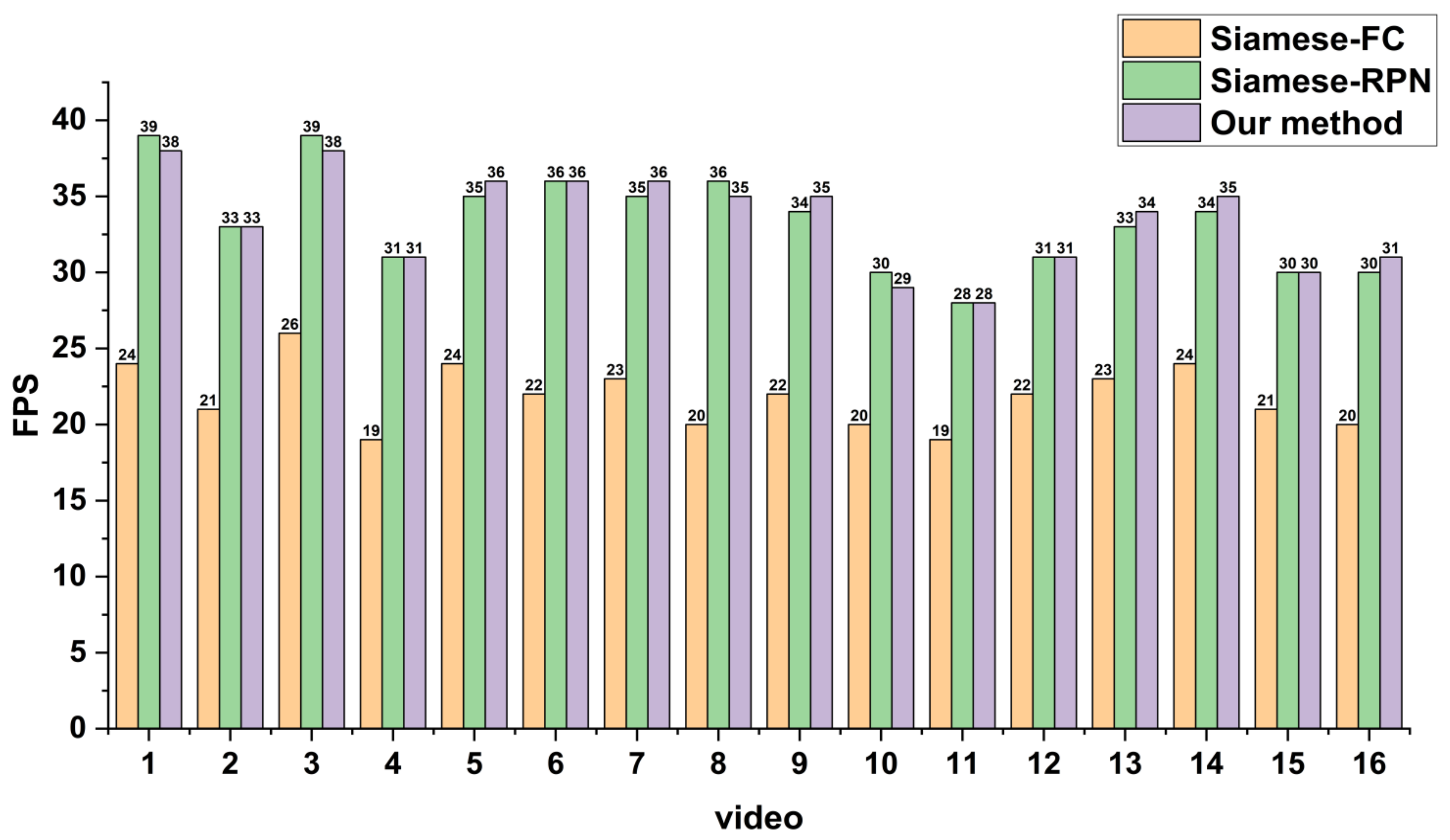
To validate the speed of GASN, we used FPS to compare GASN to Siamese-RPN and Siamese-FC. Figure 21 shows the comparison results of FPS, from which we can see that GASN (marked with purple) is almost identical to Siamese-RPN (marked with green), while Siamese-FC (marked with yellow) is lower. To the best of our knowledge, Siamese-RPN can satisfy real-time tracking [17]. Compared to Siamese-RPN, on the one hand, GASN needs to calculate the location and shape of the anchors, which reduces the tracking speed. On the other hand, the anchors are sparse, which reduces the computation of subsequent processing. It can be seen from the experimental results that the FPS of GASN is almost the same as that of Siamese-RPN; therefore, our method can achieve real-time tracking.
Table 4 shows the average tracking performance of the real Video-SAR data using the different methods. Due to the simple framework, MOSSE has the lowest performance, with 29.64% accuracy and 37.64 CLE, but the highest speed (125 FPS). Moreover, the deep learning methods improved the accuracy over the traditional correlation filtering methods (MOSSE and KCF), because the networks can extract multi-level and more expressive features. Most importantly, GA-SubNet in GASN only locates the sparse anchors containing the center of the shadow to suppress false alarms. Additionally, GA-SubNet refines the anchor’s shape to conform to the shape of the shadow, which further improves the tracking accuracy. Therefore, the accuracy of GASN (54.68%) is better than that of Siamese-RPN (52.75%) and Siamese-FC (41.60%). In addition, because the sparse anchors can reduce the subsequent computation, there is no speed loss in GASN (33 FPS) compared to Siamese-RPN (33 FPS). The above analysis shows that GASN has the highest accuracy (54.68%) without sacrificing speed.

4.2.2. Tracking Results with Clutter

To verify the suppression ability of the proposed method for clutter, we selected the videos with these two types of interference in the real data for tracking. Because Siamese-RPN has excellent performance in both accuracy and speed in optical tracking, and the proposed method is better than Siamese-RPN, making it applicable to Video-SAR, we compared the proposed method with Siamese-RPN, as shown in Figure 22. Figure 22a,b show the tracking results of the proposed GASN method and Siamese-RPN under background clutter (e.g., road signs), respectively, where the green boxes represent the ground truths of the TOI during this tracking process, and the red boxes represent the tracking results. The comparison clearly shows that the overlap between the tracking results (red) and the labels of the TOI (green) using the proposed GASN method is greater than 50%, while the overlap of Siamese-RPN is less than 30%. Figure 22c,d show the tracking results of the proposed method and Siamese-RPN under environmental clutter (e.g., imaging sidelobe), respectively, and it can be seen that the overlap between the tracking results (red) and the labels of the TOI (green) using the proposed method is higher than the results using Siamese-RPN. Therefore, we believe that the tracking accuracy of the proposed method is higher than that of Siamese-RPN in the presence of clutter.

4.2.3. Tracking Results of Different Frame Rates

Figure 23 shows the tracking results of different frame rates. We created Video 16 from Video 15 at a frame rate of 6.4, noting that the frame rate here refers to the rate at which a video is divided into frames. For example, the frame rate of Videos 1–15 was 3.2, which means that an SAR image was captured every 1/3.2 s in the video. The parameters of Video 15 in Figure 23a and of Video 16 in Figure 23b are the same, except for the frame rate. It is obvious that the two boxes in Figure 23b have higher IoUs, i.e., more accurate tracking results. Only the comparison results for frame 5 are shown, showing that the results of almost all frames in Video 16 are more accurate than those of Video 15. The main reason is that the higher the frame rate, the smaller the change in the shadow’s location and shape between the adjacent frames. Therefore, it is reasonable to assume that the frame rate is positively correlated with the tracking accuracy.

4.2.4. Tracking Results of another Real Video-SAR Dataset

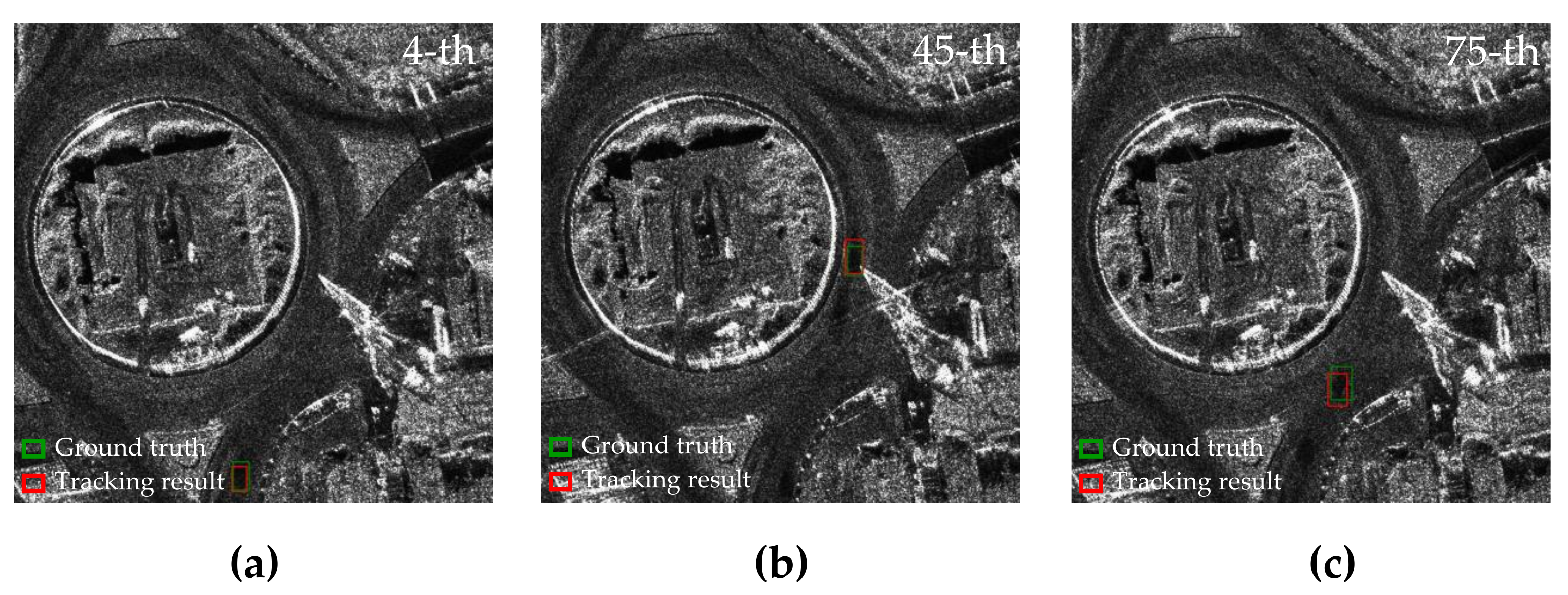
We conducted an additional experiment on a new dataset that is derived from [15]. Two videos containing 675 images were used to train the network, and two videos with 389 images were used to test the network. The size of all images was 1000 × 1000 pixels.
Figure 24 shows the tracking results of another real Video-SAR dataset, and Table 5 shows the average tracking performance. From Table 5, we can see that the accuracy of the proposed method is 1.33% higher than that of Siamese-RPN. Therefore, the proposed method is still more accurate than Siamese-RPN.

5. Discussion

5.1. Research on the Transfer

We arranged a set of experiments to verify whether the proposed method entirely relies on the prior information of the TOI, such as the location and shape, rather than the appearance features of the training data. In the first experiment, we used the simulated data for training and the real data for testing, as shown in Figure 25a,b. In the second experiment, we used the real data for training and the simulated data for testing, as shown in Figure 25c,d. We can see that the tracking results (marked with red boxes) and the ground truths of the shadow (marked with green boxes) have a great overlap in the two experiments.
To reveal the performance of GASN more intuitively, we evaluated the tracking results using accuracy, and the results are shown in Table 6 and Table 7.
The first set of cross-validation experiments involved training with real data (data B) and testing with simulated data (data A). The results are shown in row 2 of Table 6. For comparison, we also provide the results of both the training and testing using simulated data (see row 1 of Table 6). The experimental results show that their accuracy differs by 0.9%.
The second set of cross-validation experiments involved training with simulation data (data A) and testing with real data (data B). The results are shown in row 2 of Table 7. For comparison, we also provide the results of both the training and testing using real data (row 1 of Table 7). The experimental results show that their accuracy differs by 1.3%.
From the above experiments, we can see that the results of the two cross-validation experiments have little difference in terms of accuracy, which indicates that GASN has good transfer ability.
The proposed GASN in this paper is capable of similarity learning. In other words, GASN is trained with a large number of training samples so that the network has the ability to measure the similarity of two input images (i.e., the template and the search image in the training data). The greater the similarity, the higher the output score of GASN. Therefore, once a template image of TOI is given, the information provided by the template (such as the location and shape) can be used to match the target in the next image based on the similarity measure capabilities of GASN. Then, the target with the highest similarity is determined as the tracking result in the next image. Therefore, GASN can track the TOI using the template information instead of the appearance features of the training data, so the proposed GASN is highly robust.

5.2. Ablation Experiment of GA-SubNet

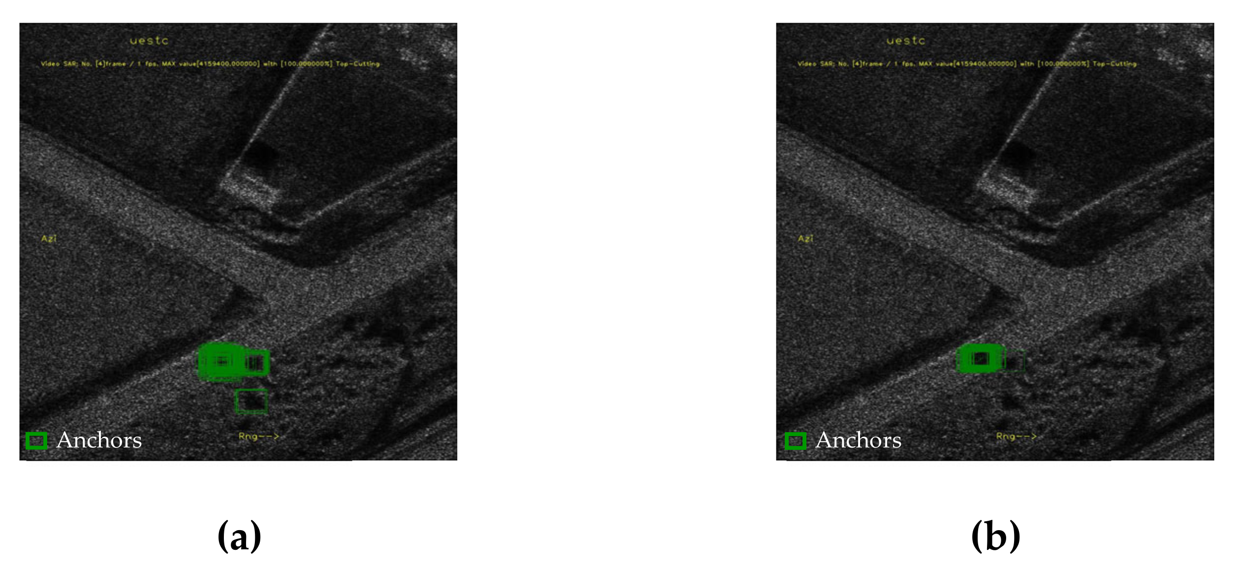
We explored the effect of GA-SubNet on false alarms. Figure 26 shows the anchors on Siamese-RPN (Figure 26a) and GASN (Figure 26b). It can be seen that after adding GA-SubNet, the anchors are mainly concentrated around the TOI, and the number of anchors is also greatly reduced. Table 8 shows the comparison results of whether to add GA-SubNet or not. Because GA-SubNet discards the useless anchors in the background and improves the imbalance between positive and negative samples, the accuracy is improved by 4.52% after adding GA-SubNet. Therefore, GASN with GA-SubNet can better distinguish the TOI from the background.

5.3. Research on Pre-Training

In the deep learning field, in recent years, a common practice is to pre-train a model on some large-scale training data [31,32,33]. As shown in Figure 6b, the one-channel SAR image needs to be copied three times to use the pre-training parameters of three-channel RGB optical images. This method of copying one-channel SAR images three times has been widely used in SAR image processing tasks [12,15]. For example, to be suitable for SAR tracking tasks, the pre-training parameters of the optical image are adjusted by the one-channel SNL data copied three times, and the tracking results are good.
To determine whether it is reasonable to apply a model trained on a three-channel RGB image to a one-channel radar image in a completely different domain or not, we arranged a group of experiments. The final tracking results for the simulated data are shown in Table 9. The second row of the results contains the tracking results after pre-training the model using optical images and then fine-tuning the training using SAR images replicated as three channels. The first row contains the tracking results after training using only replicated SAR images without pre-training with optical images. The tracking accuracy is significantly reduced by approximately 4% compared to the second row. This illustrates that it is feasible and reasonable to apply a model trained on three-channel RGB images to one-channel radar images. Therefore, it is wise to use fine-tuning in the absence of sufficient training data.

5.4. Research on the Statistical Analysis

Regarding the statistical analysis of small data, we added an experiment where we trained 10 times and calculated the statistical average (including the mean and variance of the accuracy and the central location error (CLE)). The results are shown in Table 10.
From the table, we can see that our method outperforms Siamese-RPN in terms of accuracy (58.79 > 56.37) and the accuracy variance (0.61 < 0.72), which indicates that our method is accurate and that the accuracy is more stable.
Moreover, our method outperforms Siamese-RPN in terms of the central location error (CLE) (7.49 > 6.56) and the CLE variance (0.89 < 0.98), which indicates that the CLE of our method is smaller and that the CLE is more stable.

6. Conclusions

To achieve the tracking of arbitrary TOIs in Video-SAR, this paper proposed a novel GASN. GASN is based on the idea of similarity learning, which uses the feature map of the template as the convolution kernel to slide windows on the feature map of the search image. Then, the output indicates the similarity of the two feature maps. Based on the maximum similarity, GASN can determine the tracking results in the search image. GASN tracks the TOI between the first frame and the next one instead of learning the appearance among all separate frames. Additionally, we established a GA-SubNet, which uses the location information of the template to obtain the location probability in the search image and selects the location with a probability greater than the threshold to exclude false alarms. To improve the tracking accuracy, the anchor that more closely matches the shape of the TOI is obtained by GA-SubNet through adaptive prediction processing. The experimental results showed that the tracking accuracy of the proposed method was 60.16% and 54.68% on the simulated and real Video-SAR data, respectively, which are higher than that of the two deep learning methods Siamese-RPN and Siamese-FC and the two traditional methods MOSSE and KCF.
In the future, we will try to apply scale invariant feature transform (SIFT) [34] and the Lee filter [35] to real Video-SAR for more accurate tracking results and research how to use the accurate tracking trajectory to refocus the moving target.

Author Contributions

Conceptualization, J.B. and X.Z.; methodology, J.B.; software, J.B.; validation, J.B., X.Z. and T.Z.; formal analysis, J.B.; investigation, J.B.; resources, J.S.; data curation, J.S.; writing—original draft preparation, J.B.; writing—review and editing, J.B.; visualization, X.Z.; supervision, T.Z.; project administration, X.Z.; funding acquisition, X.Z., J.S. and S.W. All authors have read and agreed to the published version of the manuscript.

Funding

This work was supported in part by the National Natural Science Foundation of China under grants 61571099, 61501098, and 61671113.

Acknowledgments

The authors thank all reviewers for their comments toward improving our manuscript, as well as the Sandia National Laboratory of the United States for providing SAR images. The authors would also like to thank Durga Kumar for his linguistic assistance during the preparation of this manuscript.

Conflicts of Interest

The authors declare no conflict of interest.

Abbreviations

SymbolDefinition
xSearch image
φ(x)Detected feature map
gSimilarity learning function
F2New detected feature map for the best anchor shape
A w × h × 4 k r e g Similarity map regression
(w, h)The weight and height of the shadow
loss loc Anchor location loss
loss cls Classification loss
PThe tracking result
( x R , y R ) The center coordinates of the tracking result
tThe total tracking time
zTemplate image
φ(z)Template feature map
F1Original detected feature map
kThe number of anchors
A w × h × 2 k c l s Similarity map for classification
(x, y)The center point of the shadow in the previous image
loss shape Anchor shape loss
loss reg Regression loss
GThe shadow’s ground truth
( x G , y G ) The center coordinates of the shadow’s ground truth
NThe number of frames of the Video-SAR sequence

References

  1. Damini, A.; Balaji, B.; Parry, C.; Mantle, V. A videoSAR mode for the X-band wideband experimental airborne radar. In Proceedings of the Algorithms for Synthetic Aperture Radar Imagery XVII, Orlando, FL, USA, 18 April 2010; p. 76990E. [Google Scholar]
  2. Wells, L.; Sorensen, K.; Doerry, R.B. Developments in SAR and IFSAR systems and technologies at Sandia National Laboratories. In Proceedings of the 2003 IEEE Aerospace Conference Proceedings (Cat. No. 03TH8652.), Big Sky, MT, USA, 8–15 March 2003; pp. 21085–21095. [Google Scholar]
  3. Hawley, R.W.; Garber, W.L. Aperture weighting technique for video synthetic aperture radar. In Proceedings of the Algorithms for Synthetic Aperture Radar Imagery XVIII, Orlando, FL, USA, 4 May 2011; p. 805107. [Google Scholar]
  4. Linnehan, R.; Miller, J.; Bishop, E.; Horndt, V. An autofocus technique for video-SAR. In Proceedings of the Algorithms for Synthetic Aperture Radar Imagery XX, Baltimore, MD, USA, 23 May 2013; p. 874608. [Google Scholar]
  5. Miller, J.; Bishop, E.; Doerry, A. An application of backprojection for Video-SAR image formation exploiting a subaperature circular shift register. In Proceedings of the Algorithms for Synthetic Aperture Radar Imagery XX, Baltimore, MD, USA, 23 May 2013; p. 874609. [Google Scholar]
  6. Wang, H.; Chen, Z.; Zheng, S. Preliminary research of low-RCS moving target detection based on Ka-band Video-SAR. IEEE Geosci. Remote Sens. Lett. 2017, 14, 811–815. [Google Scholar] [CrossRef]
  7. Henke, D.; Dominguez, E.M.; Small, D.; Schaepman, M.E.; Meier, E. Moving target tracking in single-and multichannel SAR. IEEE Trans. Geosci. Remote Sens. 2015, 53, 3146–3159. [Google Scholar] [CrossRef]
  8. Yang, X.; Shi, J.; Zhou, Y.; Wang, C.; Wei, S. Ground Moving Target Tracking and Refocusing Using Shadow in Video-SAR. Remote Sens. 2020, 12, 3083. [Google Scholar] [CrossRef]
  9. Ying, Z.; Daiyin, Z.; Xiang, Y.; Mao, X. Approach to moving targets shadow detection for VideoSAR. J. Electron. Inf. Technol. 2017, 39, 2197–2202. [Google Scholar]
  10. Zhao, B.; Han, Y.; Wang, H.; Tang, L.; Wang, T. Robust Shadow Tracking for Video-SAR. IEEE Geosci. Remote Sens. Lett. 2020, 18, 821–825. [Google Scholar] [CrossRef]
  11. Tian, X.; Liu, J.; Mallick, M. Simultaneous Detection and Tracking of Moving-Target Shadows in ViSAR Imagery. IEEE Trans. Geosci. Remote Sens. 2020, 59, 1182–1199. [Google Scholar] [CrossRef]
  12. Ding, J.; Wen, L.; Zhong, C.; Loffeld, O. Video-SAR Moving Target Indication Using Deep Neural Network. IEEE Trans. Geosci. Remote Sens. 2020, 58, 7194–7204. [Google Scholar] [CrossRef]
  13. Ren, S.; He, K.; Girshick, R.; Sun, J. Faster r-cnn: Towards real-time object detection with region proposal networks. arXiv 2015, arXiv:150601497. [Google Scholar] [CrossRef] [PubMed] [Green Version]
  14. Gers, F.A.; Schmidhuber, J.; Cummins, F.A. Learning to Forget: Continual Prediction with LSTM. Neural Comput. 2000, 12, 2451–2471. [Google Scholar] [CrossRef] [PubMed]
  15. Zhou, Y.; Shi, J.; Wang, C.; Hu, H.; Zhou, Z.; Yang, X.; Zhang, X.; Wei, S. SAR Ground Moving Target Refocusing by Combining mRe3 Network and TVβ -LSTM. IEEE Trans. Geosci. Remote Sens. 2020, 1–4. [Google Scholar] [CrossRef]
  16. Wen, L.; Ding, J.; Loffeld, O. Video-SAR Moving Target Detection Using Dual Faster R-CNN. IEEE J. Sel. Top. Appl. Earth Obs. Remote Sens. 2021, 14, 2984–2994. [Google Scholar] [CrossRef]
  17. Li, B.; Yan, J.; Wu, W.; Zheng, Z.; Hu, X. High performance visual tracking with siamese region proposal network. In Proceedings of the IEEE Conference on Computer Vision and Pattern Recognition, Salt Lake City, UT, USA, 18–23 June 2018; pp. 8971–8980. [Google Scholar]
  18. Bertinetto, L.; Valmadre, J.; Henriques, J.F.; Vedaldi, A.; Torr, P. Fully-convolutional siamese networks for object tracking. In Proceedings of the European conference on computer vision, Amsterdam, The Netherlands, 3 November 2016; pp. 850–865. [Google Scholar]
  19. Bolme, D.S.; Beveridge, J.R.; Draper, B.A.; Lui, Y.M. Visual object tracking using adaptive correlation filters. In Proceedings of the 2010 IEEE Computer Society Conference on Computer Vision and Pattern Recognition, San Francisco, CA, USA, 13–18 June 2010; pp. 2544–2550. [Google Scholar]
  20. Henriques, J.F.; Caseiro, R.; Martins, P.; Batista, J. High-speed tracking with kernelized correlation filters. IEEE Trans. Pattern Anal. Mach. Intell. 2014, 37, 583–596. [Google Scholar] [CrossRef] [PubMed] [Green Version]
  21. Tao, R.; Gavves, E.; Smeulders, A.W.M. Siamese instance search for tracking. In Proceedings of the IEEE Conference on Computer Vision and Pattern Recognition, Las Vegas, NV, USA, 26 June–1 July 2016; pp. 1420–1429. [Google Scholar]
  22. Held, D.; Thrun, S.; Savarese, S. Learning to track at 100 fps with deep regression networks. In Proceedings of the European conference on computer vision, Amsterdam, The Netherlands, 3 November 2016; pp. 749–765. [Google Scholar]
  23. Cai, Z.; Vasconcelos, N. Cascade r-cnn: Delving into high quality object detection. In Proceedings of the IEEE Conference on Computer Vision and Pattern Recognition, Salt Lake City, UT, USA, 18–23 June 2018; pp. 6154–6162. [Google Scholar]
  24. Dai, J.; Qi, H.; Xiong, Y.; Li, Y.; Zhang, G.; Hu, H.; Wei, Y. Deformable convolutional networks. In Proceedings of the IEEE International Conference on Computer Vision, Venice, Italy, 24–27 October 2017; pp. 764–773. [Google Scholar]
  25. He, K.; Zhang, X.; Ren, S.; Sun, J. Deep residual learning for image recognition. In Proceedings of the IEEE Conference on Computer Vision and Pattern Recognition, Las Vegas, NV, USA, 26 June–1 July 2016; pp. 770–778. [Google Scholar]
  26. Russakovsky, O.; Deng, J.; Su, H.; Krause, J.; Satheesh, S.; Ma, S.; Huang, Z.; Karpathy, A.; Khosla, A.; Bernstein, M. Imagenet large scale visual recognition challenge. Int. J. Comput. Vis. 2015, 115, 211–252. [Google Scholar] [CrossRef] [Green Version]
  27. Davies, D.L.; Bouldin, D.W. A cluster separation measure. IEEE Trans. Pattern Anal. Mach. Intell. 1979, 2, 224–227. [Google Scholar] [CrossRef]
  28. Lin, T.-Y.; Goyal, P.; Girshick, R.; He, K.; Dollár, P. Focal loss for dense object detection. In Proceedings of the IEEE international conference on computer vision, Venice, Italy, 24– 27 October 2017; pp. 2980–2988. [Google Scholar]
  29. Wang, J.; Chen, K.; Yang, S.; CL Chen, C.; Lin, D. Region proposal by guided anchoring. In Proceedings of the IEEE/CVF Conference on Computer Vision and Pattern Recognition, Long Beach, CA, USA, 15–20 June 2019; pp. 2965–2974. [Google Scholar]
  30. Kristan, M.; Leonardis, A.; Matas, J.; Felsberg, M.; He, Z. The visual object tracking vot2017 challenge results. In Proceedings of the IEEE International Conference on Computer Vision Workshops, Venice, Italy, 22–29 October 2017; pp. 1949–1972. [Google Scholar]
  31. Van Sloun, R.J.G.; Cohen, R.; Eldar, Y. Deep Learning in Ultrasound Imaging. Proc. IEEE 2019, 108, 11–29. [Google Scholar] [CrossRef] [Green Version]
  32. Yin, S.; Peng, Q.; Li, H.; Zhang, Z.; You, X.; Fischer, K.; Furth, S.L.; Tasian, G.E.; Fan, Y. Computer-Aided Diagnosis of Congenital Abnormalities of the Kidney and Urinary Tract in Children Using a Multi-Instance Deep Learning Method Based on Ultrasound Imaging Data. In Proceedings of the 2020 IEEE 17th International Symposium on Biomedical Imaging (ISBI), Iowa City, IA, USA, 3–7 April 2020; pp. 1347–1350. [Google Scholar] [CrossRef]
  33. Einsidler, D.; Dhanak, M.; Beaujean, P. A Deep Learning Approach to Target Recognition in Side-Scan Sonar Imagery. In Proceedings of the OCEANS 2018 MTS/IEEE Charleston, Charleston, SC, USA, 22–25 October 2018; pp. 1–4. [Google Scholar] [CrossRef]
  34. Lowe, D.G. Distinctive Image Features from Scale-Invariant Keypoints. Int. J. Comput. Vis. 2004, 60, 91–110. [Google Scholar] [CrossRef]
  35. Lopes, A.; Touzi, R.; Nezry, E. Adaptive speckle filters and scene heterogeneity. IEEE Trans. Geosci. Remote Sens. 1990, 28, 992–1000. [Google Scholar] [CrossRef]
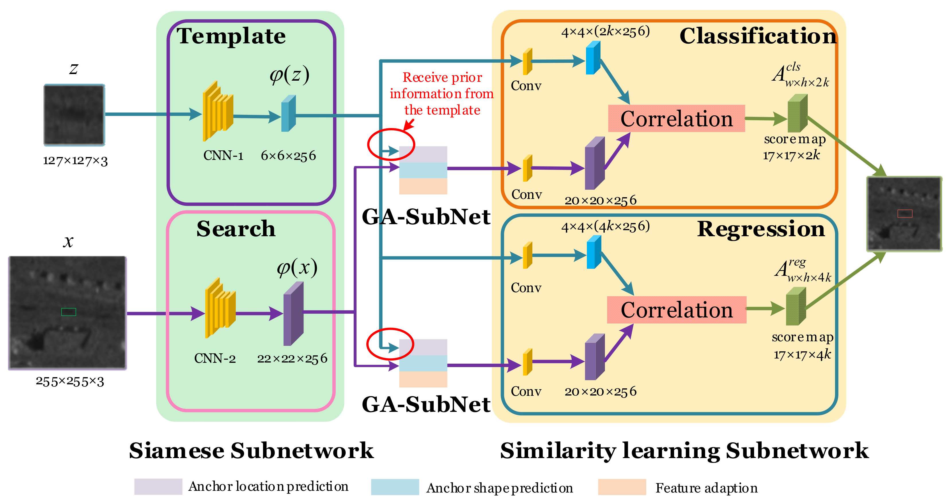
Figure 1. The architecture of GASN.
Remotesensing 13 04504 g001
Figure 2. The architecture of GA-SubNet: (a) anchor location prediction module generates the sparse location of anchors; (b) anchor shape prediction module generates the anchor shape that better conforms to the shape of the shadow; (c) feature adaptation module generates a new feature map for the best anchor shape.
Remotesensing 13 04504 g002
Figure 3. The feature composition of A w × h × 2 k cls and A w × h × 4 k reg .
Remotesensing 13 04504 g003
Figure 4. The input preprocessing of GASN.
Remotesensing 13 04504 g004
Figure 5. The whole process of arbitrary TOI tracking based on GASN.
Remotesensing 13 04504 g005
Figure 6. Image preprocessing and feature embedding. Input SAR Video (a), preprocess image (b), embed features (c).
Remotesensing 13 04504 g006
Figure 7. Predicting the anchor location.
Remotesensing 13 04504 g007
Figure 8. Predict anchor shape.
Remotesensing 13 04504 g008
Figure 9. Adapting the feature map guided by anchors.
Remotesensing 13 04504 g009
Figure 10. The tracking results obtained after comparing the similarity; comparison of the similarity of the feature maps (a), classification and regression (b), and tracking results (c).
Remotesensing 13 04504 g010
Figure 11. Image sequence of a test video: (a) third frame in Video 1; (b) 23rd frame in Video 1; (c) 43rd frame in Video 1; (d) 60th frame in Video 1.
Remotesensing 13 04504 g011
Figure 12. Tracking results of the simulated Video-SAR data: (a) 9th frame in Video 2; (b) 14th frame in Video 2; (c) 37th frame in Video 2; (d) 56th frame in Video 2.
Remotesensing 13 04504 g012
Figure 13. The comparison results of GASN with Siamese-RPN and Siamese-FC on accuracy.
Remotesensing 13 04504 g013
Figure 14. The comparison results of GASN with Siamese-RPN and Siamese-FC on CLE.
Remotesensing 13 04504 g014
Figure 15. The comparison results of GASN with Siamese-RPN and Siamese-FC on FPS.
Remotesensing 13 04504 g015
Figure 16. Tracking results with distractors: (a) TOI-1 in the 51st frame of Video 6; (b) TOI-2 in the 51st frame of Video 6.
Remotesensing 13 04504 g016
Figure 17. Tracking results of the target with a specific speed: (a) TOI-1 in the 20th frame of Video 5; (b) TOI-2 in the 20th frame of Video 5.
Remotesensing 13 04504 g017
Figure 18. Tracking results of the real Video-SAR data: (a) third frame in Video 2; (b) 35th frame in Video 2; (c) 52nd frame in Video 2.
Remotesensing 13 04504 g018
Figure 19. Accuracy comparison of the three methods.
Remotesensing 13 04504 g019
Figure 20. CLE comparison of the three methods.
Remotesensing 13 04504 g020
Figure 21. FPS comparison of the three methods.
Remotesensing 13 04504 g021
Figure 22. Tracking results with interference: (a) Siamese-RPN with background clutter; (b) our method with background clutter; (c) Siamese-RPN with environmental clutter; (d) our method with environmental clutter.
Remotesensing 13 04504 g022
Figure 23. True tracking results of different frame rates: (a) Video 15 at a frame rate of 3.2; (b) Video 15 at a frame rate of 6.4 (Video 16).
Remotesensing 13 04504 g023
Figure 24. Tracking results of another real Video-SAR data: (a) 4th frame; (b) 45th frame; (c) 75th frame.
Remotesensing 13 04504 g024
Figure 25. The experimental results of cross-validation: (a) simulated Video-SAR data for training; (b) real Video-SAR data for testing; (c) real Video-SAR data for training; (d) simulated Video-SAR data for testing.
Remotesensing 13 04504 g025
Figure 26. Ablation experiment on GA-SubNet: (a) Siamese-RPN; (b) GASN.
Remotesensing 13 04504 g026
Table 1. The system parameters of simulated Video-SAR.
ParameterValue
Center frequency/GHz
Platform velocity/m s−1
Platform height/m
35
300
8000
Pulse repetition frequency/Hz4000
Total record time/s
SNR
10
40 dB
Table 2. The velocity of the moving targets in the simulated Video-SAR data.
TargetAzimuth Velocity (m s−1)Radial Velocity (m s−1)
T16–8
T2–1–2
T31.5–3
T40.4–0.8
T531.5
T61.5–1.5
Table 3. Average tracking performance of simulated Video-SAR data.
MethodAccuracyCLEFPS
MOSSE31.21%19.76105
KCF41.80%11.3058
Siamese-FC43.67%8.4619
Siamese-RPN55.61%7.9431
GASN (ours)60.16%6.6832
Table 4. Average tracking performance of real Video-SAR data.
MethodAccuracyCLEFPS
MOSSE29.64%37.64125
KCF39.98%18.7954
Siamese-FC41.60%15.4121
Siamese-RPN52.75%14.6933
GASN (ours)54.68%11.3733
Table 5. Average tracking performance of another real Video-SAR data.
MethodAccuracyCLEFPS
MOSSE30.70%38.7365
KCF46.30%19.0358
Siamese-FC51.70%16.8121
Siamese-RPN53.68%12.0420
GASN (ours)55.01%11.7819
Table 6. Cross-validation for testing the simulated Video-SAR data.
Train DataTest DataAccuracy
SimulatedSimulated60.16%
RealSimulated59.26%
Table 7. Cross-validation for testing the real Video-SAR data.
Train DataTest DataAccuracy
RealReal54.68%
SimulatedReal53.38%
Table 8. Ablation experiment of GA-SubNet.
MethodGA-SubNetAccuracy
Siamese-RPN55.57%
GASN (ours)60.09%
Table 9. Accuracy indexes of research on pre-training.
Pre-TrainingAccuracy
56.73%
60.09%
Table 10. The statistical analysis of the tracking result.
MethodAccuracy %CLE
Siamese-RPN56.37 ± 0.727.49 ± 0.98
GASN (ours)58.79 ± 0.616.56 ± 0.89
Publisher’s Note: MDPI stays neutral with regard to jurisdictional claims in published maps and institutional affiliations.