Abstract
In this study, the harbor aquaculture area tested is Zhanjiang coast, and for the remote sensing data, we use images from the GaoFen-1 satellite. In order to achieve a superior extraction performance, we propose the use of an integration-enhanced gradient descent (IEGD) algorithm. The key idea of this algorithm is to add an integration gradient term on the basis of the gradient descent (GD) algorithm to obtain high-precision extraction of the harbor aquaculture area. To evaluate the extraction performance of the proposed IEGD algorithm, comparative experiments were performed using three supervised classification methods: the neural network method, the support vector machine method, and the maximum likelihood method. From the results extracted, we found that the overall accuracy and F-score of the proposed IEGD algorithm for the overall performance were and , meaning that the IEGD algorithm outperformed the three comparison algorithms. Both the visualized and quantitative results demonstrate the high precision of the proposed IEGD algorithm aided with the CEM scheme for the harbor aquaculture area extraction. These results confirm the effectiveness and practicality of the proposed IEGD algorithm in harbor aquaculture area extraction from GF-1 satellite data. Added to that, the proposed IEGD algorithm can improve the extraction accuracy of large-scale images and be employed for the extraction of various aquaculture areas. Given that the IEGD algorithm is a type of supervised classification algorithm, it relies heavily on the spectral feature information of the aquaculture object. For this reason, if the spectral feature information of the region of interest is not selected properly, the extraction performance of the overall aquaculture area will be extremely reduced.
1. Introduction
Given that the scientific planning of harbor aquaculture areas is an effective and sustainable way to develop fishery resources, the scientific determination of the area’s spatial distribution and the real-time monitoring of it are necessary and of critical importance. Moreover, the use of remote sensing techniques allows one to observe objects on the surface of the water through satellite images and overcome the shortcomings of traditional monitoring technology. These techniques have become an important means of dynamic monitoring in harbor aquaculture areas [1]. In recent years, some scholars have achieved excellent extraction results and application prospects in harbor aquaculture area extraction experiments, greatly promoting the development of remote sensing technology [2,3]. The state-of-the-art extraction methods used for harbor aquaculture areas can be divided into three main categories: visual interpretation methods, object-oriented methods, pixel-oriented methods, and neural network methods.
The visual interpretation method is the most commonly used extraction method [4,5]. For example, Zeng et al. used medium-resolution multispectral images for aquaculture pond extraction [6], with the results indicating that the visual interpretation method makes extraction of the target site more difficult. Furthermore, Luo et al. presented a dynamic monitoring method [7] that has important implications for future upgrades to improve aquaculture and other issues. By using Landsat images and through visual interpretation, Duan et al. identified the dynamic nature of the growth of aquaculture pond areas in coastal areas of China [8].
In general, the area provided to aquaculture ponds in most provinces initially increases rapidly and then stabilizes or begins to decline. Therefore, monitoring the extent of aquaculture areas is a matter of great urgency. Zhang et al. used GF-2 satellite images to achieve a superior extraction of aquaculture areas in turbid waters, providing technical support to the aquaculture industry [9]. However, the existence of visual interpretation relies on the visual interpreter’s own experience, which is not conducive to the monitoring needs of aquaculture areas because of the large and time-consuming workload involved.
Next, the object-oriented extraction method comprehensively considers the space, spectrum, texture, and shape features of classified objects in remote sensing images [10,11,12]. To demonstrate the advantages of this method, Peng et al. used the CBR (Case-Based Reasoning) method [13] to successfully accomplish the segmentation of multi-scale images to complete classification and extraction. The process of object-oriented pond culture information extraction consists of image preprocessing, edge extraction, image segmentation, feature analysis, and extraction, etc. [14]. Liu et al. [14] and Xu et al. [15] further optimized the object-oriented extraction technique to improve the classification accuracy [15] while quantitatively describing the change in sea area usage in the study area.
In addition, Wei integrated visual interpretation with the object-oriented approach to optimize the classification and extraction accuracy, thus, optimizing the object-oriented extraction [16]. However, the object-oriented approach also possesses non-negligible drawbacks, such as different types of features presenting the same spectral characteristics in a certain spectral interval, leading to their incorrect classification.
Additionally, the pixel-oriented extraction method can make good use of the spectral reflection characteristics of the aquaculture area and use the threshold to extract the aquaculture area automatically [17]. This was confirmed in the research of Hussain et al. [18] and Zheng el al. [19]. Affected by different water quality factors in the same culture area, the reflection characteristics of aquaculture areas differ, making the pixel-oriented extraction method more difficult to perform. In addition, the setting of the extraction threshold in the pixel-oriented extraction method also needs to be specified manually. When the aquaculture extraction range becomes large, it is difficult to select the threshold that will produce the best extraction results. All these factors make it difficult for the pixel-oriented extraction method to extract aquaculture areas independently and accurately.
With the development of deep learning, more neural networks are being applied for the monitoring of aquaculture areas. The reason for this is that neural networks have shown excellent capabilities in the areas of automated processing, self-learning, and parsing in complex environments. Therefore, in order to achieve the monitoring and extraction of aquaculture areas using neural networks, Cui et al. identified the shortcomings of visual interpretation and proposed a method based on the automatic extraction of floating raft culture areas using a fully convolutional neural network (CNN) model [20], which effectively improved the accuracy of floating raft culture area identification.
Moreover, Jiang et al. upgraded the CNN model to a 3D-CNN model [21], which is an extraction model with a high extraction accuracy and strong spatial migration ability in complex water backgrounds. Therefore, the presented model is suitable for extracting large-scale, multi-temporal offshore rafting areas from remote sensing images. Further, Liu et al. used GF-2 satellite images to construct a deep learning richer convolutional feature network model for the water and soil separation of areas [3], thus achieving effective extraction in areas with more sediment and waves.
On top of that, Cheng et al. provided a hybrid dilated convolution U-Net model [22], indicating that their method possesses excellent distinguishability. In addition, Fu et al. constructed a hierarchical cascaded homogeneous neural network for marine aquaculture extraction. This network showed a superior classification performance to that of other existing methods [23]. However, in the above neural network algorithms, it can be seen that they all require a certain number of training samples and take a long time, making them very unfavorable for large-scale image observation.
After the above explanations and analyses, this paper aims to address the matter of aquaculture extraction with a generalizable performance, simple operation, explicit implementation, and high accuracy. For this reason, an implementable and feasible constrained energy minimization (CEM) scheme for aquaculture extraction is considered. Moreover, combined with the actual application effect of remote sensing based on satellite images and the actual demands of the Zhanjiang aquaculture area, this research selected GF-1 satellite PMS images as the data source. It is important to bear in mind that gradient-type algorithms have been proven to possess an accessible implementation paradigm for use in various optimization problems.
Therefore, in order to further improve the extraction accuracy of the CEM scheme in aquaculture areas, this paper proposes the use of an integrated-enhanced gradient descent (IEGD) algorithm derived from the gradient descent (GD) algorithm. The innovations made by this work are as follows. The proposed IEGD algorithm is derived from a major innovation in control theory, which adds an integration error summation term to improve the computational precision. In other words, the integration error summation term can effectively eliminate the deviation between the computed and theoretical solutions. In general, the proposed IEGD algorithm demonstrates highly accurate extraction results in aquaculture areas. The main contributions and highlights are summarized as follows:
- 1.
- Based on control theory, the proposed IEGD algorithm represents a major breakthrough of the traditional gradient descent algorithm for solving extraction problems and can be regarded as a novel algorithmic paradigm.
- 2.
- The proposed IEGD algorithm possesses relatively excellent robustness.
- 3.
- The proposed IEGD algorithm improves the shortcomings of the traditional CEM algorithm with an insufficient accuracy.
2. Research Principles and Methods
2.1. Technical Route
In view of the complex and diverse spectra of remote sensing images of objects on the ground in the research area, the method proposed in this paper is mainly divided into three stages—namely, spectral feature selection, an IEGD solving algorithm, and ground object extraction. First of all, this paper uses the feature index method and the Bhattacharyya Distance (BD) method to screen the sensitive wavebands to form the spectral feature set. Secondly, the CEM scheme aided by the proposed IEGD algorithm is used to enhance the target ground object and weaken the background spectral information. Finally, Otsu’s method is used to calculate the division threshold to achieve ground object extraction. Figure 1 shows the technical route map.
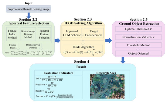
Figure 1.
Technical route of harbor aquaculture area extraction.
2.2. Spectral Feature Selection
Due to the different reflection characteristics of ground objects in different wave bands, the characteristic index method can be used to amplify the small brightness differences and highlight the spectral characteristics of ground objects. For situations where there is a high chlorophyll concentration and high suspended sediment content in Zhanjiang nearshore waters, the NDWI (Normalized Difference Water Index) feature index,
is applied in this study [24] to reduce the influence of chlorophyll and suspended sediment on aquaculture area information.
After the above band expansion method has been applied, the new bands (NDWI) are obtained as well as the blue, green, red, and near-infrared bands of the GF-1 image for a total of 17 wavebands. These wavebands contain not only the characteristic information of the surface features in the culture area, but also the information of suspended sediment and chlorophyll concentration in non-culture waters. However, not all bands are sensitive to the target ground objects in the culture area.
In order to eliminate the band information that has a weak relation to the target ground object, we analyze the spectral characteristics of ground objects and use the Bhattacharyya Distance to screen the bands. Bhattacharyya Distance measurement determines the similarity of two discrete or continuous probability distributions by comparing the overlap between species in order to analyze the similarity between two statistical samples or populations [25].
where represents the mean value of the gray-level eigenvalues of two different ground objects and is the standard deviation between ground objects. The larger the BD value is, the greater the spectral difference between the ground objects is, and the easier it is to distinguish. In this study, all the above seven bands were screened using the Bhattacharyya Distance method, three bands with great differences from the ground objects were retained, and a band feature set for the ground object was formed using band synthesis technology.
Table 1 shows the BD ratios of each waveband, where , and represent the gray-level values of GF-1 satellites from blue, green, red, and near infra-red bands after atmospheric correction.

Table 1.
The BD ratio of each waveband.
Combined with the spectral characteristics of the ground objects in the culture area, we can see that the spectral difference between the cage and the sea water in the raft culture area is the smallest. Thus, the BD value between the cage and the sea water is selected as the selection standard of the spectral feature set in the raft culture area. Therefore, the spectral feature set of the raft culture zone is mainly composed of , , and the near-infrared band.
2.3. IEGD Solving Algorithm
The Constrained Energy Minimization (CEM) scheme [26] is a classical hyperspectral image target detection algorithm that is widely used in the field of remote sensing image ground object extraction [27,28,29]. The traditional CEM scheme regards the input remote sensing image as a limited observation signal set and supposes that a hyperspectral image can be arranged as a matrix , where each column of S is a spectral vector and is a spectral vector representing the spectrum of targets of interest. In this, N is the number of pixels and l is the number of wavebands. The CEM scheme designs a finite impulse response (FIR) linear filter under the assumption that the prior information d of the target pixel spectrum is known and minimizes the average output “energy” of the image under the constraint of the following formula:
where is the filter coefficient, which is a l-dimensional vector. Suppose the output of the filter to input is :
Then, the average output “energy” corresponding to can be written as:
where is the autocorrelation matrix of the remote sensing image and represents the output “energy” of each pixel in the image after passing through the filer. Therefore, the CEM scheme can be described as a linearly constrained optimization mathematical model as follows:
By using the Lagrange multiplier method, the linearly constrained optimization mathematical model (4) of the filter output can be transformed into an unconstrained optimization mathematical model as follows:
where is the Lagrangian multiplier. The mathematical model of unconstrained optimization (5) is transformed into a mathematical model of linear equality equation as follows:
where the autocorrelation coefficient matrix , the coefficient vector , is the unsolved vector, is the l-dimensional vector composed of filter coefficients, and is the Lagrangian function multiplier. Then, the error function that defines Equation (6) is as follows:
In order to better solve for the CEM scheme (3), we must define a scalar-valued norm-based error function,
where represents the Frobenius norm of matrix G. Moreover, denotes the trace operator of a matrix. Additionally, a lemma that we must know [30] is:
Finally, the formula follows the form shown above:
Combined with the algorithm mentioned above, the gradient descent algorithm can be obtained as:
According to automatic control theory, adding an integration error summation term to Formula (9) can increase the robustness of this formula:
Finally, the discrete form of the integration-enhanced gradient descent (IEGD) algorithm is constructed as follows:
where k denotes the iteration number. Through recursive calculation, the filter output coefficient obtained is inverted, and thus the aquaculture area target enhancement process is completed. Furthermore, the pseudo-algorithm of the proposed IEGD algorithm (10) is provided as Algorithm 1:
| Algorithm 1: IEGD algorithm solving procedure. |
| 1. Initial set , , , , , b, R, and d |
| 2. Circular iteration |
| for (; k ; ) do |
|
calculate calculate calculate calculate calculate end for |
| 3. Output |
2.4. Theoretical Analyses
In this section, the convergence performance of the proposed model will be discussed at zero noise.
2.4.1. Conversion
In order to prove the convergence performance more conveniently, Equation (11) should be transformed. First, multiply matrix G on both sides:
Based on the matrix theory, the real symmetric matrix can then be generated:
where is the eigenvalue of the positive definite matrix and the symbol ≃ denotes the similarity of the two matrices. In line with above derivation, Equation (11) can be transformed:
where . Based on Equation (7), Equation (13) can be simplified to:
where denotes the member of a vector, , and .
2.4.2. Stability Analyses
Theorem 1.
For a randomly generated initial state of the proposed IEGD algorithm (10), the residual error converges to zero globally.
Proof of Theorem 1.
Take the element arbitrarily from Equation (14) as a subsystem where:
Define a Lyapunov for Equation (15). This can be:
Then, begin the derivation of the constructed Lyapunov function (16):
Therefore, based on the Lyapunov theory, it can be concluded that converges to zero globally. In summary, the theorem has been proven. □
2.4.3. Convergence Analyses
Theorem 2.
Proof.
Let . Combining this with Equation (15), Equation (15) can be rewritten as:
We arrange the above equation as:
According to the solution of the differential equation, two feature roots can be obtained as:
After that, in order to solve this differential Equation (18), initial values of and are given. There are three situations in Equation (18), which are discussed as follows:
- , where , i.e., .For the solution of , can be written as:Combining the above formulas, can be obtained:
- , where —i.e., .For the solution of , can be written as:Combining the above formulas, can be obtained:
- , where , i.e., .The solution of the , can be written as:Combining the above formulas, can be obtained
Based on the above three situations and according to the conclusion of Theorem 1, it can be concluded that the convergence speed converges exponentially to the conclusion from Theorem 1. In summary, the proof of this theorem is completed. □
2.5. Ground Object Extraction
Otsu’s method mainly divides the image into a target and background according to the gray-level difference of the image and determines the optimal threshold by obtaining the inter-class variance between the ground objects. The algorithm is efficient and fast, and the execution efficiency is high [31,32]. The calculation formula is as shown in (19), where and are the probability that the image pixels are divided into the target pixels and the background pixels and and are the average gray-level values of the image pixels divided into target pixels and the background pixels.
The enhanced remote sensing image is used to calculate the division threshold using Otsu’s method. In this process, because the overall gray level of some sea water pixels is similar to that of aquaculture objects, it is mistakenly categorized as the area of aquaculture features to improve the false detection rate of aquaculture areas. Therefore, aiming at the sea water retention phenomenon, this study used the characteristic that the gray-level value of sea water in a single band is smaller than that of cultured objects and carried out single-band threshold segmentation.
In view of the fact that the gray value of the sea water pixels in the raft culture area in the blue waveband is smaller than that in the cage, after many experiments, the blue waveband gray threshold and the near-red waveband gray threshold are used as the single-band threshold values in the raft culture area to segment the sea water and the raft. The preliminary extraction effect of the raft culture area is better, as the raft culture area separates most of the sea water from the raft, leaving only a small part of the high-turbidity water at the edge of the coast.
It is difficult to remove this water because the suspended sediment is too high. Finally, we use the object-oriented area attributes to remove the sea water. In this process, sea water with an area smaller than 43 pixels or larger than 700 pixels is removed to obtain the final extraction result.
3. Materials
3.1. Research Area
As shown in Figure 2, Zhanjiang is located on Leizhou Peninsula—the third largest peninsula in China, at the southernmost tip of the Chinese mainland. It is also an important aquaculture base for Guangdong Province and even for China [33]. The research object of this paper is mainly the raft culture area, which is divided into aquaculture rafts for oyster culture and cages for captive fish culture. Aquaculture rafts are mainly composed of bamboo or wood, and there is often a rope hanging down from the aquaculture raft to cultivate shellfish, such as oysters.
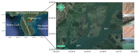
Figure 2.
The research area in true color with image examples are raft and cage aquaculture areas on the satellite (a1 and b1, respectively) and ground (a2 and b2, respectively).
In the process of culturing, the rafts are closely arranged, the oysters cling onto the rope and are immersed in the water, and only the aquaculture raft floats on the water surface, showing a bright white rectangular object on the remote sensing image, as shown in Figure 2. The cage is usually composed of wooden boards and plastic buckets, and there are small fish ponds inside, which are shown as a rectangular grid similar to the color of the water in remote sensing images, as shown in Figure 2.
3.2. Data Sources
The GF-1 satellite is the first high-resolution and wide-width Earth observation satellite developed by China Aerospace Science and Technology Corp. The highest spatial resolution of the satellite is 2 meters (m), and the maximum imaging width is more than 800 kilometers (km), meaning that it can meet the needs of remote sensing data with various spatial and spectral resolutions [34,35]. The GF-1 PMS level 1 data are made up of five wavebands—namely, one panchromatic band and four multispectral wavebands [35]. The specific parameters are shown in Appendix A Table A1.
The ENVI (Environment for Visualizing Images) 5.3 software is used to preprocess the remote sensing images, performing radiometric calibration, atmospheric correction, orthophoto correction, and so on. At the same time, in order to identify the culture area in the image more clearly, the GS (Gram–Schmidt) method is used to fuse the multi-spectral and panchromatic images, thus improving the spatial resolution of the multi-spectral image to 2 meters (m).
3.3. Accuracy Evaluation
In order to evaluate the accuracy of the detection results, the overall accuracy (OA), precision, recall, and F-score are used. The OA, precision, recall, and F-score are computed as follows [36]:
where TP denotes, if the true category of the sample is a positive case and the model predicts it to be a positive case; TN denotes, if the true category of the sample is a negative case and the model predicts it to be a negative case; FP denotes, if the true category of the sample is a negative case but the model predicts it to be a positive case; FN denotes, if the true category of the sample is a positive case but the model predicts it to be a negative case [37], and represents the weight. When , this indicates that both precision and recall are important.
4. Result
In this section, we apply five extraction methods in the study region to compare their performance and judge the accuracy of their extraction rafts against the accuracy mentioned above. The five methods are the integration-enhanced gradient descent (IEGD) algorithm (10), the constrained energy minimization (CEM) scheme (3), neural network (NN) [38], support vector machine (SVM) [39], and maximum likelihood estimation (MLE) [40], which are presented in this paper. In addition, Figure 3 represents the original image of the study area.
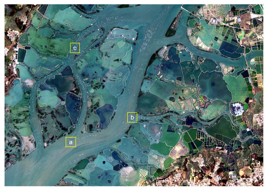
Figure 3.
The research area, where a, b, c denotes three regions of study areas and the white color represents the aquaculture rafts.
4.1. Results of the Extraction Process
Not counting the time spent on image preprocessing in the ENVI software, the time taken to run the Algorithm 1 of the IEGD algorithm (10) in Matlab 2017A was seconds. This time was less than two seconds for a large-scale image with pixels and 2-meter spatial resolution. It is worth noting that all the experiments were performed using MATLAB 2017A and ENVI 5.3 on a computer with Windows 10, the AMD Ryzen 5 3600 6-Core Processor @3.60 GHz and 32 GB RAM. In addition, certain results of the extraction process are shown below:
where d is the prior information, is the filter coefficient, is the optimal threshold, and R is the autocorrelation matrix of the remote sensing image.
4.2. Overall Performance
First, Figure 3 shows the original image of the whole raft breeding area, where the white color represents the aquaculture rafts. Figure 4 shows the graph of the results after extraction has been carried out using the IEGD algorithm (10). Table 2 represents the comparison of the accuracy evaluation of various methods in the whole raft culture. From the overall view, the extraction effect is very satisfactory, basically extracting all the aquaculture rafts. This is demonstrated by the F-scores given in Table 2, which are above 0.96. Furthermore, it is necessary to explore the extraction accuracy of various methods locally.
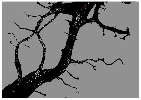
Figure 4.
The IEGD algorithm (10) is applied to extract rafts from the whole study area, where white denotes rafts, black denotes sea water, gray denotes land, red denotes the missing extraction, and green denotes greater extraction.
Table 2.
Comparison of the accuracy evaluation index of various methods in raft farming areas, where OA denotes the ratio of the predicted correct result samples to the total samples, precision denotes the ratio of the actual positive samples to the predicted positive samples, recall denotes the ratio of the predicted positive samples to the actual positive samples, and the F-score is a combined consideration of the precision and recall.
4.3. Local Performance
In this subsection, we will apply five extraction methods in three different regions, of which this region is the region mentioned in the previous subsection. We will compare the performance of these five extraction methods and judge the accuracy of their extraction of rafts against the accuracy mentioned above. Table 3 indicates the different accuracies of these five methods in different regions. In the following pictures of the comparison of different regional methods, there will be three different colors, where green stands for misclassified aquaculture areas, red stands for omitted aquaculture areas, and black represents the background.
Table 3.
The accuracy evaluation index of the use of various methods in different regions, where OA denotes the ratio of the predicted correct result samples to the total samples, precision denotes the ratio of actual positive samples to predicted positive samples, recall denotes the ratio of the predicted positive samples to the actual positive samples, and the F-score is a combined consideration of the precision and recall.
4.3.1. Region a
In Region a, we can clearly observe that the proposed IEGD algorithm (10) possesses superior performance in the extraction of Region a. It can be clearly seen in Figure 5 that only the proposed IEGD algorithm (10) neither misses aquaculture rafts nor misidentifies other objects that are not aquaculture rafts as aquaculture rafts. In the accuracy for each method in each region in Table 3, it is clear that the accuracy of the proposed IEGD algorithm (10) is above 0.97, while the accuracies of the rest of the methods are worse to different degrees.
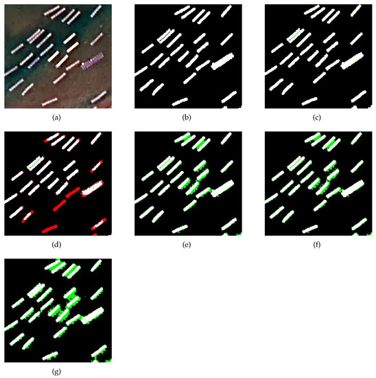
Figure 5.
Details of the results of aquatic product extraction carried out by different methods in Region a with a black color denoting background, white color denoting the aquaculture raft, red color denoting the missing extraction, and green color denoting more extraction. (a) Original image. (b) Ground truth image. (c) IEGD (10). (d) CEM (3). (e) NN [38]. (f) SVM [39]. (g) MLE [40].
In terms of details, although the overall extraction accuracy of the IEGD algorithm (10) is the best, in terms of recall, MLE [40] performs better and exhibits no missed extraction. However, because of the defects of this method, it results in the lowest precision rate among the five methods, at 0.6484. In turn, it can be demonstrated in Table 3 that the precision and recall rates of the proposed IEGD algorithm (10) are 0.9907 and 0.9767, respectively, while the F-score value of 0.9837 demonstrates the excellence of this algorithm. Therefore, in Region a, the proposed IEGD algorithm (10) performs the best out of the five algorithms.
4.3.2. Region b
Figure 6 shows the image information of Region b. Due to there being less interference in the image information, the correct extraction accuracy of these five methods rebounded compared to that obtained in region a. The extraction performance of the proposed IEGD algorithm (10) is still excellent; it can perfectly extract the rafts in this region, and its accuracy is above 0.99. Compared with Region a, its general accuracy OA is improved except for MLE.
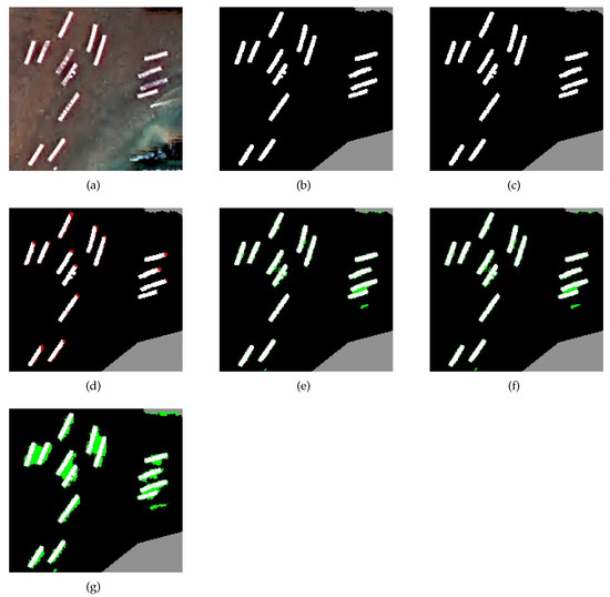
Figure 6.
The details of the results of aquatic product extraction by different methods in Region b, with a black color denoting the background, white color denoting the aquaculture raft, red color denoting the missing extraction, and green color denoting more extraction. (a) Original image. (b) Ground truth image. (c) IEGD. (d) CEM. (e) NN. (f) SVM. (g) MLE.
Compared with Region a, the range missed by the CEM scheme (3) was drastically reduced, while, for NN [38], the SVM [39] misjudgment was also significantly reduced. This is because the CEM scheme (3) still maintains a very high precision of 0.9978, while that of the proposed IEGD algorithm (10) differs by only 0.0059. However, in terms of recall, the CEM scheme (3) differs from the other methods by more than 0.1, which is a large error. Nevertheless, the proposed IEGD algorithm (10) achieved a recall of 0.9980, representing a difference of only 0.0020 from the remaining three methods. According to the overall F-score, the proposed IEGD algorithm (10) still performs well.
4.3.3. Region c
The accuracy of Region c decreased compared to that of Regions a and b. This is most likely due to the fact that the rafts in this region are too dense with cargo as well as with interference from some objects. As shown in Table 3, the accuracy of all methods decreased. Surprisingly, there is no difference between the accuracy of the proposed IEGD algorithm (10) and that of the CEM scheme (3).
However, in the raft extraction of region c, there is a missed extraction and a false extraction. The accuracy of SVM [39] surpasses that of the CEM scheme (3) at 0.9995, but its recall is the lowest among these five methods, at only 0.7537. In terms of recall, MLE [40] is the best without exception, achieving a recall of 0.9993. In terms of combined precision and recall, the proposed IEGD algorithm (10) and CEM scheme (3) perform the best in region c extraction.
5. Discussion
5.1. Robustness Discussion
- 1.
- From the viewpoint of optimization theory, the proposed IEGD algorithm (10) and the other four compared methods are supervised learning classification algorithms that are considered as optimization models. Differing from the others, the proposed IEGD algorithm (10) improves the model computing accuracy and enhances the model robustness by adding an integration error summation term, which can be supported by the stability analysis and convergence analysis described in Section 2.4.2 and Section 2.4.3.
- 2.
- Our proposed method should also be discussed from the viewpoint of experimental results. The three representative Regions a, b, and c all show the phenomena of “same object with different spectra” and “same spectrum with different objects”. These are undoubtedly the best testing examples for evaluating the robustness performance of the actual extraction effectiveness. According to the corresponding visual and quantitative results shown in Figure 4, Figure 5, Figure 6 and Figure 7 and Table 2 and Table 3, the robustness of the proposed IEGD algorithm (10) is the best.
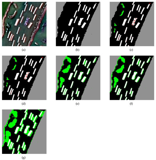 Figure 7. The details of the results of aquatic product extraction by different methods in Region c, with a black color denoting the background, white color denoting the aquaculture raft, red color denoting the missing extraction, and green color denoting more extraction. (a) Original image. (b) Ground truth image. (c) IEGD. (d) CEM. (e) NN. (f) SVM. (g) MLE.
5.2. Applicability Discussion
- 1.
- The proposed IEGD algorithm (10) makes full use of the spectral, textural, and spatial geometric feature information of the Zhanjiang offshore aquaculture area and increases the feature dimension of aquatic image elements in the aquaculture area by constructing various feature indexes. Moreover, the proposed IEGD algorithm (10) enhances the target feature information in the aquaculture area, making the difference between the aquaculture objects and non-aquaculture objects more distinct. The proposed IEGD algorithm (10) can better expand the feature information between the target object and background object to improve the performance of supervised learning classification, allowing it to effectively overcome the phenomena of “same object with different spectra” and “same spectrum with different objects”.This algorithm is relatively reliable in cases where there are rich spectral features and a high extraction accuracy. It can be used as a self-selected algorithm for extracting aquaculture areas from high-resolution remote sensing images. In cases where there are fewer spectral features, it can also be combined with other existing methods to achieve a satisfying extraction performance.
- 2.
- Differing from most existing extraction methods that only focus on local small areas, the proposed IEGD algorithm (10) can be directly employed for large-scale remote sensing images and can achieve an overall extraction of full-frame images.
- 3.
- The proposed IEGD algorithm (10) is an important breakthrough for supervised learning classification algorithms, which is attributed to the integrated processing of the Matlab and ENVI software. When processing large-scale remote sensing images, the use of this algorithm can guarantee the accuracy of local feature extraction and provide a fast extraction speed. This can be seen in the extraction results of the experimental process. Not counting the time spent on image preprocessing in the ENVI software, the time generally taken to run the Algorithm 1 of the proposed IEGD algorithm (10) in Matlab 2017A is s.This time is less than two seconds for a large-scale image with pixels and a 2-meter spatial resolution. In addition, the overall accuracy and F-score of the proposed IEGD algorithm (10) in terms of the overall performance are and , meaning that it outperforms the other four comparison algorithms. This demonstrates the excellent extraction performance of the proposed algorithm in aquaculture areas.
5.3. Expansibility Discussion
- 1.
- The proposed IEGD algorithm (10) belongs to the category of optimization methods. Specifically, it improves the traditional gradient descent method by introducing an integration error summation term to help its optimal solution process and obtain a higher-precision computational solution. In this way, the proposed algorithm can be extended to other remote sensing-like algorithms that are applicable to the gradient descent method to help improve their solution accuracy. It is well known that the gradient descent method is a widely used algorithm in application scenarios; thus, the proposed IEGD algorithm (10) possesses high expansibility, good implementability, and acceptable feasibility.
- 2.
- The proposed IEGD algorithm (10) is currently used for single aquaculture objects (i.e., rafts), but it can be extended to multiple aquaculture object extraction tasks by adding the prior spectral information of multiple targets.
- 3.
- The proposed IEGD algorithm (10) can not only be employed for GF-1 remote sensing images but also for other multi-source remote sensing images, especially hyperspectral remote sensing images.
- 4.
- The proposed IEGD algorithm (10) can be used not only for extraction from aquaculture objects but also for other areas, such as mining areas, surface water on land, crops, etc.
5.4. Limitations
- 1.
- The proposed IEGD algorithm (10) relies heavily on the spectral features of the aquaculture features as prior information and still lacks the ability to fully exploit and utilize the local image element dependencies. As a result, some preprocessing of the remote sensing images of the aquaculture features is needed in order to render the spectra features sufficiently reliable.
- 2.
- Supervised learning classification requires the manual selection of regions of interest (ROI), which can be easily influenced by manual subjectivity.
- 3.
- For supervised learning classification, our algorithm can only determine the ROI in defined regions that have been manually selected. It relies on human subjective selectivity and can easily miss some tiny regions, leading to a significant reduction in the extraction performance for the overall aquaculture area.
6. Conclusions
In this study, taking the offshore raft culture area of Zhanjiang City, Guangdong province, as the research object, we used domestic high-resolution GF-1 PMS images as the data source; studied the extraction rules for raft farming areas in high-resolution remote sensing images; and proposed an IEGD algorithm (10) that combines spectral features of remote sensing image features, the threshold method, etc. The neural network method, support vector machine method, and maximum likelihood estimation of traditional supervised classification methods were compared with the proposed IEGD algorithm (10) in this paper.
The results show that, even in culture areas where the phenomenon of “foreign bodies with the same spectrum” is obvious, this method can effectively overcome the interference of background ground objects and obtain high-precision raft culture area extraction results. Compared with supervised classification, the overall accuracy of this method is more than 0.98. At the same time, for the extraction of other ground objects (including different crops and other types of culture areas), it is expected that this method will also provide a better application effect.
In addition, through the research in this paper, the IEGD algorithm (10) can better help others to observe the distribution of rafts in the farming area, which makes the layout of the farming area reasonable. The limitation of this paper is that the IEGD algorithm (10) relies on the spectral information of the farming features as a priori information to be extracted, which happens to be a great drawback. Since the a priori information needs to be selected manually, subjective human judgment is extremely important. Applying this method to more areas and improving it will be subjects of our future work.
Author Contributions
Conceptualization, D.F. and G.Y.; methodology, Y.Z. and S.L.; software, Y.Z. and G.Y.; validation, Y.Z. and D.F.; writing—original draft preparation, Y.Z.; writing—review and editing, Y.Z. and G.Y.; visualization, H.H.; project administration, D.F.; funding acquisition, D.F. All authors have read and agreed to the published version of the manuscript.
Funding
This research was funded by Key Projects of the Guangdong Education Department (2019KZDXM019); Southern Marine Science and Engineering Guangdong Laboratory (Zhanjiang) (ZJW-2019-08); High-Level Marine Discipline Team Project of Guangdong Ocean University (00202600-2009); First Class Discipline Construction Platform Project in 2019 of Guangdong Ocean University (231419026); Guangdong Graduate Academic Forum Project (230420003); Postgraduate Education Innovation Project of Guangdong Ocean University (202159); Provincial-Level College Student Innovation and Entrepreneurship Training Project (S202110566052).
Data Availability Statement
Not applicable.
Acknowledgments
The authors would like to thank the anonymous reviewers and editors for their valuable comments and suggestions on earlier versions of the manuscript.
Conflicts of Interest
The authors declare no conflict of interest.
Appendix A
Table A1.
Parameters of GF-1 PMS multi-spectral satellite images.
Table A1.
Parameters of GF-1 PMS multi-spectral satellite images.
| Band Order | Value (m) | Spatial Resolution (m) |
|---|---|---|
| Pan 1-Panchromatic | 0.450–0.900 | 2 |
| Band 1-Blue | 0.450–0.520 | 8 |
| Band 2-Green | 0.520–0.590 | 8 |
| Band 3-Red | 0.630–0.690 | 8 |
| Band 4-NIR | 0.770–0.890 | 8 |
References
- Ma, Y.; Chen, F.; Liu, J.; He, Y.; Duan, J.; Li, X. An Automatic Procedure for Early Disaster Change Mapping Based on Optical Remote Sensing. Remote Sens. 2016, 8, 272. [Google Scholar] [CrossRef] [Green Version]
- Sui, B.; Jiang, T.; Zhang, Z.; Pan, X.; Liu, C. A Modeling Method for Automatic Extraction of Offshore Aquaculture Zones Based on Semantic Segmentation. ISPRS Int. J. Geo-Inf. 2020, 9, 145. [Google Scholar] [CrossRef] [Green Version]
- Liu, Y.; Yang, X.; Wang, Z.; Lu, C.; Li, Z.; Yang, F. Aquaculture Area Extraction and Vulnerability Assessment in Sanduao Based on Richer Convolutional Features Network Model. J. Oceanol. Limnol. 2019, 37, 1941–1954. [Google Scholar] [CrossRef]
- Hoekstra, M.; Jiang, M.; Clausi, D.A.; Duguay, C. Lake Ice-Water Classification of RADARSAT-2 Images by Integrating IRGS Segmentation with Pixel-Based Random Forest Labeling. Remote Sens. 2020, 12, 1425. [Google Scholar] [CrossRef]
- Bey, A.; Sánchez-Paus Díaz, A.; Maniatis, D.; Marchi, G.; Mollicone, D.; Ricci, S.; Bastin, J.F.; Moore, R.; Federici, S.; Rezende, M.; et al. Collect Earth: Land Use and Land Cover Assessment through Augmented Visual Interpretation. Remote Sens. 2016, 8, 807. [Google Scholar] [CrossRef] [Green Version]
- Zeng, Z.; Wang, D.; Tan, W.; Huang, J. Extracting Aquaculture Ponds from Natural Water Surfaces around Inland Lakes on Medium Resolution Multispectral Images. Int. J. Appl. Earth Obs. Geoinf. 2019, 80, 13–25. [Google Scholar] [CrossRef]
- Luo, J.; Pu, R.; Ma, R.; Wang, X.; Lai, X.; Mao, Z.; Zhang, L.; Peng, Z.; Sun, Z. Mapping Long-Term Spatiotemporal Dynamics of Pen Aquaculture in a Shallow Lake: Less Aquaculture Coming along Better Water Quality. Remote Sens. 2020, 12, 1866. [Google Scholar] [CrossRef]
- Duan, Y.; Tian, B.; Li, X.; Liu, D.; Sengupta, D.; Wang, Y.; Peng, Y. Tracking Changes in Aquaculture Ponds on the China Coast Using 30 Years of Landsat Images. Int. J. Appl. Earth Obs. Geoinf. 2021, 102, 102383. [Google Scholar] [CrossRef]
- Zhang, X.; Ma, S.; Su, C.; Shang, Y.; Wang, T.; Yin, J. Coastal Oyster Aquaculture Area Extraction and Nutrient Loading Estimation Using a GF-2 Satellite Image. IEEE J. Sel. Top. Appl. Earth Obs. Remote Sens. 2020, 13, 4934–4946. [Google Scholar] [CrossRef]
- Benz, U.C.; Hofmann, P.; Willhauck, G.; Lingenfelder, I.; Heynen, M. Multi-Resolution, Object-Oriented Fuzzy Analysis of Remote Sensing Data for GIS-Ready Information. ISPRS J. Photogramm. Remote Sens. 2004, 58, 239–258. [Google Scholar] [CrossRef]
- Tan, Z.; Zhang, Z.; Xing, T.; Huang, X.; Gong, J.; Ma, J. Exploit Direction Information for Remote Ship Detection. Remote Sens. 2021, 13, 2155. [Google Scholar] [CrossRef]
- Fu, Y.; Deng, J.; Ye, Z.; Gan, M.; Wang, K.; Wu, J.; Yang, W.; Xiao, G. Coastal Aquaculture Mapping from Very High Spatial Resolution Imagery by Combining Object-Based Neighbor Features. Sustainability 2019, 11, 637. [Google Scholar] [CrossRef] [Green Version]
- Liu Peng, D.Y. A CBR Approach for Extracting Coastal Aquaculture Area. Remote Sens. Technol. Appl. 2012, 27, 857. [Google Scholar]
- Liu, F.; Shi, Q.Q.; Fei, X.Y. Object-Oriented Remote Sensing for the Variation of Sea Area Utilization. J. Huaihai Inst. Technol. (Natural Sci. Ed.) 2015, 24, 82–86. [Google Scholar]
- Xu, J.; Zhao, J.; Zhang, F.; Li, F. Object-Oriented Information Extraction of Pond Aquaculture. Remote Sens. Land Resour. 2013, 1, 82–85. [Google Scholar]
- Wei, Z. Analysis on the Relationship between Mangrove and Aquaculture in Maowei Sea Based on Object-Oriented Method. In E3S Web of Conferences; EDP Sciences: Les Ulis, France, 2020; p. 03022. [Google Scholar]
- Ma, Y.; Zhao, D.; Wang, R.; Su, W. Offshore Aquatic Farming Areas Extraction Method Based on ASTER Data. Trans. Chin. Soc. Agric. Eng. 2010, 26, 120–124. [Google Scholar]
- Hussain, M.; Chen, D.; Cheng, A.; Wei, H.; Stanley, D. Change Detection from Remotely Sensed Images: From Pixel-Based to Object-Based Approaches. ISPRS J. Photogramm. Remote Sens. 2013, 80, 91–106. [Google Scholar] [CrossRef]
- Zheng, Y.; Wu, J.; Wang, A.; Chen, J. Object- and Pixel-Based Classifications of Macroalgae Farming Area with High Spatial Resolution Imagery. Geocarto Int. 2018, 33, 1048–1063. [Google Scholar] [CrossRef]
- Cui, B.G.; Zhong, Y.; Fei, D.; Zhang, Y.H.; Liu, R.J.; Chu, J.L.; Zhao, J.H. Floating Raft Aquaculture Area Automatic Extraction Based on Fully Convolutional Network. J. Coast. Res. 2019, 90, 86–94. [Google Scholar] [CrossRef]
- Jiang, Z.; Ma, Y. Accurate extraction of Offshore Raft Aquaculture Areas Based on a 3D-CNN Model. Int. J. Remote Sens. 2020, 41, 5457–5481. [Google Scholar] [CrossRef]
- Cheng, B.; Liang, C.; Liu, X.; Liu, Y.; Ma, X.; Wang, G. Research on a Novel Extraction Method Using Deep Learning Based on GF-2 Images for Aquaculture Areas. Int. J. Remote Sens. 2020, 41, 3575–3591. [Google Scholar] [CrossRef]
- Fu, Y.; Deng, J.; Wang, H.; Comber, A.; Yang, W.; Wu, W.; You, S.; Lin, Y.; Wang, K. A new satellite-derived dataset for marine aquaculture areas in China’s coastal region. Earth Syst. Sci. Data 2021, 13, 1829–1842. [Google Scholar] [CrossRef]
- Ronghua, M.; Jingfang, D. Quantitative Estimation of Chlorophyll-a and Total Suspended Matter Concentration with Landsat ETM Based on Field Spectral Features of Lake Taihu. J. Lake Sci. 2005, 2, 97–103. [Google Scholar] [CrossRef] [Green Version]
- Ben Ayed, I.; Punithakumar, K.; Li, S. Distribution Matching with the Bhattacharyya Similarity: A Bound Optimization Framework. IEEE Trans. Pattern Anal. Mach. Intell. 2015, 37, 1777–1791. [Google Scholar] [CrossRef] [PubMed]
- Duan, Y.; Li, X.; Zhang, L.; Chen, D.; Ji, H. Mapping National-Scale Aquaculture Ponds Based on the Google Earth Engine in the Chinese Coastal Zone. Aquaculture 2020, 520, 734666. [Google Scholar] [CrossRef]
- Beiranvand Pour, A.; Park, Y.; Crispini, L.; Läufer, A.; Kuk Hong, J.; Park, T.Y.S.; Zoheir, B.; Pradhan, B.; Muslim, A.M.; Hossain, M.S.; et al. Mapping Listvenite Occurrences in the Damage Zones of Northern Victoria Land, Antarctica Using ASTER Satellite Remote Sensing Data. Remote Sens. 2019, 11, 1408. [Google Scholar] [CrossRef] [Green Version]
- Xi, Y.; Ji, L.; Geng, X. Pen Culture Detection Using Filter Tensor Analysis with Multi-Temporal Landsat Imagery. Remote Sens. 2020, 12, 1018. [Google Scholar] [CrossRef] [Green Version]
- Zhao, R.; Shi, Z.; Zou, Z.; Zhang, Z. Ensemble-Based Cascaded Constrained Energy Minimization for Hyperspectral Target Detection. Remote Sens. 2019, 11, 1310. [Google Scholar] [CrossRef] [Green Version]
- Zhang, Y.; Chen, K.; Tan, H.Z. Performance Analysis of Gradient Neural Network Exploited for Online Time-Varying Matrix Inversion. IEEE Trans. Autom. Control 2009, 54, 1940–1945. [Google Scholar] [CrossRef]
- Yao, S.; Chang, X.; Cheng, Y.; Jin, S.; Zuo, D. Detection of Moving Ships in Sequences of Remote Sensing Images. ISPRS Int. J. Geo-Inf. 2017, 6, 334. [Google Scholar] [CrossRef] [Green Version]
- Cao, J.; Chen, L.; Wang, M.; Tian, Y. Implementing a Parallel Image Edge Detection Algorithm Based on the Otsu-Canny Operator on the Hadoop Platform. Comput. Intell. Neurosci. 2018, 2018, 3598284. [Google Scholar] [CrossRef] [Green Version]
- Fu, D.; Zhong, Y.; Chen, F.; Yu, G.; Zhang, X. Analysis of Dissolved Oxygen and Nutrients in Zhanjiang Bay and the Adjacent Sea Area in Spring. Sustainability 2020, 12, 889. [Google Scholar] [CrossRef] [Green Version]
- Wang, J.; Jiang, L.; Wang, Y.; Qi, Q. An Improved Hybrid Segmentation Method for Remote Sensing Images. ISPRS Int. J. Geo-Inf. 2019, 8, 543. [Google Scholar] [CrossRef] [Green Version]
- Guo, H.; He, G.; Jiang, W.; Yin, R.; Yan, L.; Leng, W. A Multi-Scale Water Extraction Convolutional Neural Network (MWEN) Method for GaoFen-1 Remote Sensing Images. ISPRS Int. J. Geo-Inf. 2020, 9, 189. [Google Scholar] [CrossRef] [Green Version]
- Goutte, C.; Gaussier, E. A probabilistic interpretation of precision, recall and F-score, with implication for evaluation. In European Conference on Information Retrieval; Springer: Berlin/Heidelberg, Germany, 2005; pp. 345–359. [Google Scholar]
- Lewis, H.; Brown, M. A Generalized Confusion Matrix for Assessing Area Estimates from Remotely Sensed Data. Int. J. Remote Sens. 2001, 22, 3223–3235. [Google Scholar] [CrossRef]
- Fu, Y.; Ye, Z.; Deng, J.; Zheng, X.; Huang, Y.; Yang, W.; Wang, Y.; Wang, K. Finer Resolution Mapping of Marine Aquaculture Areas Using WorldView-2 Imagery and a Hierarchical Cascade Convolutional Neural Network. Remote Sens. 2019, 11, 1678. [Google Scholar] [CrossRef] [Green Version]
- Zhang, H.; Jiang, Q.; Xu, J. Coastline Extraction Using Support Vector Machine from Remote Sensing Image. J. Multim. 2013, 8, 175–182. [Google Scholar]
- Han, J.; Chi, K.; Yeon, Y. Aquaculture Feature Extraction from Satellite Image Using Independent Component Analysis. In Proceedings of the International Workshop on Machine Learning and Data Mining in Pattern Recognition, Leipzig, Germany, 9–11 July 2005; Perner, P., Imiya, A., Eds.; Springer: Berlin/Heidelberg, Germany, 2005; pp. 660–666. [Google Scholar]
Publisher’s Note: MDPI stays neutral with regard to jurisdictional claims in published maps and institutional affiliations. |
© 2021 by the authors. Licensee MDPI, Basel, Switzerland. This article is an open access article distributed under the terms and conditions of the Creative Commons Attribution (CC BY) license (https://creativecommons.org/licenses/by/4.0/).