Abstract
To acquire the enhanced underwater ship-radiated noise signal in the presence of array shape distortion in a passive sonar system, the phase difference of the line-spectrum component in ship-radiated noise is often exploited to estimate the time-delay difference for the beamforming-based signal enhancement. However, the time-delay difference estimation performance drastically degrades with decreases of the signal-to-noise ratio (SNR) of the line-spectrum component. Meanwhile, although the time-delay difference estimation performance of the high-frequency line-spectrum components is generally superior to that of the low-frequency one, the phase difference measurements of the high-frequency line-spectrum component often easily encounter the issue of modulus 2 ambiguity. To address the above issues, a novel time-frequency joint time-delay difference estimation method is proposed in this paper. The proposed method establishes a data-driven hidden Markov model with robustness to phase difference ambiguity by fully exploiting the underlying property of slowly changing the time-delay difference over time. Thus, the phase difference measurements available for time-delay difference estimation are extended from that of low-frequency line-spectrum components in a single frame to that of all detected line-spectrum components in multiple frames. By jointly taking advantage of the phase difference measurements in both time and frequency dimensions, the proposed method can acquire enhanced time-delay difference estimates even in a low SNR case. Both simulation and at-sea experimental results have demonstrated the effectiveness of the proposed method.
1. Introduction
Beamforming-based signal enhancement is a crucial problem in array signal processing, and plays a significant role in feature extraction and target recognition [1,2,3,4]. In a passive sonar system, an important topic is to acquire the enhanced underwater ship-radiated noise signal from the received data of the hydrophone array [5,6,7]. A large aperture is often required to achieve accurate localization and high array gain [8,9]. The large aperture is typically formed by trailing a hydrophone array behind a towing platform in a nominally straight line [10,11]. However, the array is often deformed or distorted due to inevitable oceanic currents, hydrodynamics, and tactical maneuvers of the towing platform, resulting in time-delay mismatch in beamforming-based signal enhancement, which seriously degrades the signal enhancement performance [12,13,14,15].
Over the past several decades, a tremendous amount of effort has been devoted to time-delay difference estimation in the distorted towed hydrophone array. One intuitive method is to install the compasses and depth sensors at several points within the towed array, providing localized horizontal and vertical information on the transverse displacements of the array, respectively [11,16]. Although this type of method can acquire the array shape straightforwardly, the limited accuracy and information update rate of these auxiliary sensors make it difficult to accurately estimate the array shape in real-time [17,18]. The generalized cross-correlation (GCC) estimator, consisting of a pair of prefilters and a cross-correlator, determines the time-delay difference by locating the peak of the cross-correlator output [19,20]. Note that the towed array with a large aperture mainly focuses on the weak targets. However, the correlation between the wideband components of ship-radiated noise signals received by different hydrophones decreases significantly in the low signal-to-noise ratio (SNR) scenario, drastically degrading the time-delay difference estimation performance of the GCC method [21,22].
Line-spectrum components generated from the inevitable vibration of mechanical equipment, such as the diesel generator and air conditioning system, are a quite important and useful element in the underwater ship-radiated noise signal [23,24]. Generally, the power of the line-spectrum components is at least 10 dB higher than that of their nearby continuous spectrum such that the line-spectrum components are ready to be detected and recognized [25]. The phases of these relatively strong line-spectrum components involve the information of time-delays from the target to hydrophones, and thus can be exploited to estimate the time-delay difference of the radiated noise signal received by different hydrophones. The methods developed in [26,27] detect the line-spectrum components by locating the peaks of the power spectrum of the received acoustic signal. An adaptive discrete-time nonlinear frequency locked-loop filter is properly designed to extract the line-spectrum components from the acquired acoustic signal [28,29]. The method in [6] first modeled the line-spectrum components as the superposition of sinusoidal signals and narrow-band noise, then estimated the time-delay difference of each line-spectrum component utilizing the phase difference measurement, and finally averaged the results to acquire the final time-delay difference estimates. The minimum time-delay difference estimation variance using a sinusoidal signal with unknown frequency has been derived in [30]. The method in [31] regarded the time-delay difference as the slope of the regression line of the phase difference and applied regression analysis to acquire the time-delay differences estimates. Note that first, the accuracy of time-delay difference estimation exploiting phase difference of line-spectrum component is sensitive to noise, and drastically degrades with decreases of the SNR of the line-spectrum component [3]. Furthermore, regarding the line-spectrum components with the same SNR, the time-delay difference estimation accuracy is proportional to the frequency of the line-spectrum component, i.e., the estimation accuracy of the high-frequency line-spectrum component outperforms that of the low-frequency one [30]. However, for the phase difference measurements of high-frequency line-spectrum component whose half-wavelength is less than the inter-hydrophone spacing, there often exists the issue of modulus 2 ambiguity. If one ignores the phase difference ambiguity and still estimates the time-delay exploiting the wrapped phase difference measurements, the resulting time-delay estimates deviate from the truth values significantly. The algorithms mentioned above estimate the time-delay difference utilizing the unambiguous low-frequency line-spectrum phase difference measurement from a single frame, and thus require a relatively high SNR to achieve satisfactory performance. Unfortunately, this requirement cannot be met for the underwater ship-radiated noise signal due to the development of the vibration control and noise suppression techniques [5] resulting in a much weaker radiated noise level. Moreover, the phase difference measurements are acquired in each hydrophone element without any array gain [3].
Several improved algorithms have been proposed to acquire the enhanced time-delay difference estimates. For example, an effective outlier-robust Kalman smoother (WORKS) method has been developed in [3] to acquire enhanced time-delay estimates by exploiting the properties of slowly changing time-delay difference in the hydrophone array. This method can alleviate the effects of the outliers resulting from the diverse noise levels in the multiple line-spectrum components. Chinese remainder theorem (CRT) has been reformulated to improve the time-delay difference estimation accuracy by unwrapping the phase difference measurements of line-spectrum components [32,33,34,35,36,37]. This type of method was used to determine an integer (multiple of the time-delay difference) from its remainders (wrapped and noisy phase difference measurements) of several moduli (wavelengths of the line-spectrum components) [32]. For the conventional CRT, a small error in the remainder may cause a large error in the solution of an integer [33]. A robust CRT and its fast implementation have been proposed to reduce the reconstruction error caused by the remainder error [34,35]. In addition, a maximum likelihood estimation-based robust CRT has been developed to address the scenario when the remainder noises do not have the same variance [36]. However, the CRT-based methods have to choose the frequency of the line-spectrum component properly to ensure that there is a positive integer such that the products of this positive integer and the wavelengths of different line-spectrum components are coprime [37]. This is difficult for a passive sonar system since the frequency of line-spectrum components in ship-radiated noise is random, rather than designed artificially. The least-squares phase unwrapping estimator (LSPUE) converted the phase unwrapping problem into the problem of finding the nearest points in a lattice and solved the problem utilizing the lattice point theory in the least-squares sense [38,39]. Unfortunately, a relatively high SNR is required to achieve a satisfying phase unwrapping success rate. Overall, time-delay difference estimation exploiting phase difference measurements of line-spectrum components of the underwater ship-radiated noise signal is still an open problem for beamforming-based signal enhancement in the presence of array shape distortion, particularly in the low SNR case.
In this paper, a novel time-frequency joint time-delay difference estimation method is proposed for signal enhancement in the distorted towed hydrophone array. Unlike these conventional methods, which estimate the time-delay difference utilizing only the unambiguous low-frequency line-spectrum phase difference measurements in a single frame, the proposed method is able to acquire enhanced time-delay difference estimates by fully exploiting phase difference measurements of all detected line-spectrum components in the multiple frames. First, the line-spectrum detection is performed on the pre-enhanced signal based on the hypothetical linear array. Then, a technology combining weighted least-square (WLS) and hidden Markov model (HMM) is developed to obtain the coarse time-delay difference estimates utilizing the unambiguous phase difference measurements of low-frequency line-spectrum components. Next, a data-driven HMM robust to phase difference ambiguity is established to acquire the refined time-delay difference estimates exploiting the phase difference measurements of all detected line-spectrum components. Finally, beamforming based on the refined time-delay difference estimates is employed to achieve the signal enhancement. The performance of the proposed method is verified by both numerical simulations and at-sea experiments. The contributions of the proposed method are summarized as follows.
- (1)
- A data-driven HMM with robustness to phase difference ambiguity is established to acquire enhanced time-delay difference estimates by taking advantage of the underlying property of slowly changing time-delay difference over time;
- (2)
- The phase difference measurements available for time-delay difference estimation are extended from that of low-frequency line-spectrum components in a single frame to that of all detected line-spectrum components in multiple frames;
- (3)
- The signal enhancement performance of the proposed method with a distorted array is close to that of the existing approach with a known array shape, even if the SNR of all the line-spectrum components is as low as 4 dB.
The remainder of this paper is organized as follows. Section 2 introduces the signal model. Section 3 analyses the method for time-delay difference estimation exploiting the phase difference of line-spectrum components. The proposed time-frequency joint time-delay difference estimation method is presented in Section 4. Simulation and experiment results are provided in Section 5. Section 6 concludes the paper.
2. Signal Model
In this section, we first introduce the signal model for underwater ship-radiated noise received by a distorted towed hydrophone array, then present the problem of signal enhancement in the presence of array shape distortion.
2.1. Signal Model of Underwater Ship-Radiated Noise in Distorted Towed Hydrophone Array
Consider a flexible cable with M omnidirectional hydrophones mounted at a fixed spacing d. Because of oceanic currents, hydrodynamics, and tactical maneuvers of the towing platform, the hydrophone array towed behind a maneuvering platform cannot be kept as a straight line [11], as shown in Figure 1. Suppose that the array shape distortion only occurs on the horizontal plane [40]. Take the position of the hydrophone nearest from the platform as the origin of the coordinate system. The hydrophone in the distorted array is denoted by red circles in Figure 1 as opposed to that in the original linear array denoted by blue squares.
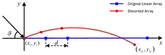
Figure 1.
Shape distortion of a towed hydrophone array.
Suppose that an underwater acoustic noise signal radiated by a far-field source impinges on the towed array with an incident angle , which is defined as the angle between the incident direction and the negative x-axis, as shown in Figure 1. The data received by the hydrophone can be expressed as
where represents the waveform of the radiated noise signal received by the reference hydrophone, denotes the time-delay of the signal propagating from the reference hydrophone to the hydrophone, and is the additive noise uncorrelated with the signal, respectively. When the first hydrophone is taken as the reference, is given by
where represents the coordinates of the hydrophone, and c denotes the sound speed in water.
The spectrum of the received hydrophone data can be written as
where , , and represent the spectrum of , , and , respectively. According to the statistical model of the underwater ship-radiated noise [24], the spectrum can be decomposed into three components, i.e.,
where represents the stationary continuous spectrum originated from the hydrodynamic noise, denotes the modulation spectrum caused by the propeller noise, and is the line-spectrum generated by the machinery noise, respectively. The machinery noise , generated from the inevitable vibration of mechanical equipment such as diesel generator and air conditioning system, is generally denoted by the collection of multiple sinusoidal signals, i.e., [3],
where , , and represent the amplitude, frequency, and initial phase of the sinusoidal signal, and K denotes the number of the sinusoidal signals. Thus, the machinery noise is also termed as the line-spectrum components of the ship-radiated noise.
2.2. Beamforming-Based Signal Enhancement in the Presence of Array Shape Distortion
Beamforming-based signal enhancement has been widely used in passive sonar systems to acquire the enhanced underwater ship-radiated noise signal from the received data of the hydrophone array [13,25]. It can be written as
where represents the estimate of the time-delay. As indicated by (6), the effect of signal enhancement depends on the estimation accuracy of the time-delay. Specifically, when the estimated time-delay is coinciding with the true time-delay , the source signal received by various hydrophones of the towed array are coherently summed. On the contrary, noise is incoherently summed when the noise in different hydrophones are uncorrelated. Consequently, the SNR of the source signal in the enhanced signal is M times that of the one in the received hydrophone data [41]. According to (2), the estimate of the time-delay can be given by
where denotes the estimate of the target direction. As indicated by (7), the exact coordinates of each hydrophone in the array are required to estimate the time-delay accurately. However, it is difficult to obtain the exact coordinates for a distorted towed array. If one ignores the array shape distortion and estimates the time-delay based on the hypothetical uniform linear array instead, i.e.,
the resulting time-delay estimates deviate from the truth values significantly. Thus, the performance of the beamforming-based signal enhancement degrades severely.
Generally, the power of the line-spectrum components in ship-radiated noise is at least 10 dB higher than that of their nearby continuous spectrum. Thus, the line-spectrum components are readily to be detected and recognized [25], as shown in Figure 2. According to (3) and (5), the phase difference of the line-spectrum component between the and hydrophones is
where represents the phase of the line-spectrum component of the radiated noise signal received by the hydrophone, is the time-delay difference of the radiated noise signal between the and hydrophones for , and . The relation between time-delay and time-delay difference is given by
It is noted from (9) and (10) that the time-delay required for beamforming-based signal enhancement can be acquired from the phase differences of line-spectrum components in the underwater ship-radiated noise signal.
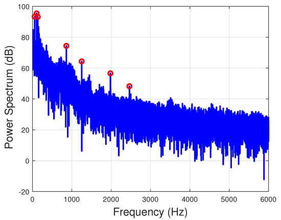
Figure 2.
The power spectrum of real radiated noise signal.
3. Time-Delay Difference Estimation Exploiting Phase Difference of Line-Spectrum Components of Underwater Ship-Radiated Noise
In this section, we first introduce the time-delay difference estimation utilizing phase difference of line-spectrum components in underwater ship-radiated noise. Then, we analyze the performance degradation caused by modulus 2 ambiguity in phase difference measurement of the high-frequency line-spectrum component.
To acquire the spatial gain of the hydrophone array, we pre-enhance the ship-radiated noise signal exploiting conventional beamforming (CBF) based on the hypothetical uniform linear array, i.e.,
where represents the sample of with a sampling rate , and N denotes the number of samples in a single frame of observation. Suppose that K line-spectrum components are detected from the power spectrum of the pre-enhanced signal, and the estimated frequency of the line-spectrum component is denoted as for .
The received hydrophone data with can be decomposed into N narrow-band frequency bins using discrete Fourier transform. The frequency bin containing the line-spectrum component can be approximately modeled as the superposition of the sinusoidal signal and narrow-band noise [3]. Exploiting maximum likelihood, the phase estimation for the line-spectrum component received by the hydrophone can be expressed as [42]
The corresponding probability density function can be expressed as [43]
where represents the right-tail integral of the standard Gaussian distribution, and denotes the SNR of the line-spectrum component received by the hydrophone, which is defined as the power ratio of the sinusoidal signal to the narrow-band noise with a bandwidth , i.e.,
where is the power spectral density at frequency of the additional noise received by the hydrophone.
According to (9), the phase difference measurement of the line-spectrum component between the and hydrophones is given by
where represents the actual phase difference, denotes the noise in phase difference measurement, is termed noisy phase difference, is an integer to ensure that , respectively. It is noted from (15) that the obtained phase difference measurement is the result of the noisy phase difference modulo 2. When the obtained phase difference measurement is unambiguous, i.e., or , time-delay difference estimation utilizing phase difference measurement of the line-spectrum component is given by
where and denote the estimation error of and , respectively. It can be noted in (16) that, for a given , the time-delay difference estimation error is proportional to the estimation errors of both phase difference and frequency of the line-spectrum component, and is inversely proportional to the frequency of the line-spectrum component. The variance of is approximately given by [30]
where represents the estimate for SNR of the line-spectrum component in the pre-enhanced signal.
Note that the detected line-spectrum components generally have diverse SNRs and frequencies. To accurately estimate the time-delay difference exploiting the phase difference measurements of all detected line-spectrum components, we can apply WLS on the phase difference measurements, i.e.,
where the superscript w denotes WLS. Substituting (17) into (18) yields the approximated variance of the WLS time-delay difference estimation, i.e.,
The estimator in (18) is optimal in terms of minimizing the sum of squared errors, when there is no modulus 2 ambiguity in phase difference measurements of all detected line-spectrum components, i.e., or for .
As indicated by (16), for the line-spectrum components with the same SNR, the time-delay difference estimation accuracy is proportional to the frequency of the line-spectrum component. However, for the line-spectrum component with frequency larger than , the absolute value of the actual phase difference may larger than . Thus, the obtained phase difference measurement is ambiguous and wrapped by 2 radians, i.e., and . In the remaining parts of this paper, unless otherwise stated, the line-spectrum component with a frequency larger than is termed high-frequency line-spectrum component, otherwise termed low-frequency line-spectrum component. If one ignores the phase difference ambiguity and still estimates the time-delay difference according to (18) exploiting the wrapped phase difference measurements, the resulted time-delay difference estimation accuracy degrades significantly. Figure 3 shows the time-delay difference estimation results utilizing phase difference measurements from line-spectrum components with frequencies of 30 Hz, 120 Hz, and 480 Hz. It can be noted that, although the time-delay difference estimates obtained from the line-spectrum component with a frequency of 480 Hz have a smaller fluctuation compared to those obtained from the line-spectrum components with frequencies of 30 Hz and 120 Hz, they exhibit significant deviations from the actual values.
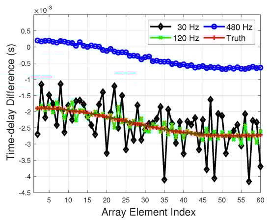
Figure 3.
Time-delay difference estimation exploiting phase difference measurements of line-spectrum components with different frequencies. All the SNRs of the line-spectrum components are 15 dB. M = 60, d = 5 m.
In addition, note that the phase difference measurement of the line-spectrum component is sensitive to noise. Moreover, the time-delay difference estimation performance degrades significantly in the low SNR case. Thus, a relatively high SNR is required to achieve satisfactory time-delay difference estimation accuracy, which is difficult in practice, as discussed in Section 1. Therefore, time-delay difference estimation exploiting phase difference measurements of line-spectrum components of the underwater ship-radiated noise signal is still an open problem for beamforming-based signal enhancement in the presence of array shape distortion, particularly in the low SNR case.
4. Proposed Time-Frequency Joint Time-Delay Difference Estimation Method for Signal Enhancement in the Distorted Towed Hydrophone Array
In this section, we propose a time-frequency joint time-delay difference estimation method to obtain the enhanced time-delay difference estimates in the low SNR case. First, we reformulate the HMM for time-delay difference estimation in Section 4.1. Then, we show the proposed method in detail, which is divided into two stages, i.e., the coarse estimation stage in Section 4.2 and the fine estimation stage in Section 4.3. Next, we summarized our scheme for signal enhancement in the distorted towed hydrophone array in Section 4.4. Eventually, we analyze the calculation complexity of the proposed method in Section 4.5.
4.1. HMM for Time-Dealy Difference Estimation
Note that the time-delay difference for ship-radiated noise signal received by adjacent hydrophones of a towed array always changes slowly and continuously. Thus, it is reasonable to model the change of time-delay difference as a first-order hidden Markov process. The HMM is characterized by , where , , and represent the state transition probability matrix, observation probability matrix, and initial state probability vector, respectively [44,45]. Let denote the set of L hidden states (time-delay differences). is uniformly distributed over with an interval for , where and represent the lower and upper bounds of the hidden states, respectively. The dimension for the set of hidden states is given by
where rounds up to an integer. The state sequence with length T is denoted as , and is the time-delay difference state at frame t for . The observation sequence is represented by , and is the observation obtained at frame t.
The state transition probability matrix is denoted as , where represents the probability of the state transitioning to at frame t when the state is at frame , i.e.,
The state equation of can be expressed as
where represents the change in time-delay difference between adjacent observations, which is an unknown non-random variable determined by the change rate of the target direction, denotes the state noise caused by the random change for the positions of target and hydrophones, and is assumed to be normally distributed with mean zero and variance . The element of is consequently given by
where is a scaling factor to ensure that satisfies for . The observation probability matrix is denoted as , where represents the probability of observing given that the state is at frame t, i.e.,
The initial state probability vector is denoted as , where denotes the probability of the starting state being , which is defined as
Generally, there is no prior information about the time-delay difference at the starting stage of signal enhancement in the presence of array shape distortion. Hence, is assumed to be uniformly distributed over , i.e., for .
To obtain the time-delay difference estimation using HMM, we need to determine the state sequence that maximizes the conditional probability function given the model . Therefore, the estimates of time-delay difference (optimal state sequence) is obtained by
which can be efficiently computed utilizing a dynamic programming method called the Viterbi algorithm [46,47] as presented in Appendix A. The obtained time-delay difference estimates are denoted as .
4.2. Coarse Time-Delay Difference Estimation
The proposed method contains two stages, i.e., the coarse and fine estimation stages, present in this and the next subsection, respectively. In the coarse estimation stage, the observation is the WLS time-delay difference estimation exploiting the unambiguous phase difference measurements from low-frequency line-spectrum components, i.e., . According to (18), is given by
where represents the WLS estimation of time-delay difference at frame t, , , and denote the estimate of frequency, SNR, and phase difference for the line-spectrum component at frame t, T stands for the number of frames (observation sequence length), and is the number of the detected low-frequency line-spectrum components, respectively. According to (19), the estimated variance of is approximately given by
Then, the lower and upper bounds of the hidden states can be set as
The interval of the hidden states can be set as
which is small enough to reduce the impact of time-delay difference discretization on estimation accuracy to a negligible level. It can be seen from (20) and (28)–(30) that the dimension for the set of the hidden states of HMM is a function of the observation sequence length and the number, frequency, and SNR of the line-spectrum components.
Although the value of time-delay difference change varies from time to time, it can be approximately regarded as a constant value within a short time. Therefore, when the window length of data fitting is set to be , the estimate of utilizing least-square linear fitting is given by
where denotes the mean of WLS time-delay difference estimation results within the sliding window. Then, the state transition probability matrix can be acquired according to (23). As for the observation probability matrix, it is given by
when is assumed to follow a Gaussian distribution.
After acquiring the HMM parameters for the coarse estimation stage as the methods described above, we can perform the Viterbi algorithm to estimate the time-delay difference. The resulted estimates of time-delay difference are denoted as (the superscript c denotes coarse).
4.3. Fine Time-Dealy Difference Estimation
Once the coarse time-delay difference estimates are obtained, the HMM parameters for the fine estimation stage of the proposed method can be acquired as follows. The lower and upper bounds of the hidden state can be set as
The interval of the hidden state is related to all detected line-spectrum components and can be set as
After updating the estimate of according to (31) utilizing the coarse time-delay difference estimates , the state transition probability matrix can be obtained according to (23).
Unlike the coarse estimation stage, where the observation sequence is the WLS time-delay difference estimates from the unambiguous phase difference measurements of low-frequency line-spectrum components, the observation sequence in the fine estimation stage is the phase difference measurements of all detected line-spectrum components, i.e., . Thus, the element of the observation probability matrix is given by
In (35), it is assumed that the phase difference measurements for different line-spectrum components are independent of each other. According to (9) and (12), the phase difference is a function of and , and the estimation of and are mutually independent. Thus, the conditional probability of the phase difference measurement can be obtained by calculating the marginal probability density function with respect to , i.e.,
More specifically, it is given by
where
Note that the conditional probability obtained in (37) associates the wrapped phase difference measurement with the actual time-delay difference. Furthermore, it is independent of the modulus 2 ambiguity of the phase difference measurements due to the cosine operation shown in (38). Therefore, the data-driven HMM established in the fine estimation stage is robust to phase difference ambiguity, and can be adopted to estimate the time-delay difference from the phase difference measurements of all detected line-spectrum components.
After obtaining the HMM parameters for the fine estimation stage, we can perform the Viterbi algorithm to estimate the time-delay difference. The resulted refined estimates of time-delay difference are denoted as (the superscript r denotes refined).
4.4. Summary of the Signal Enhancement in the Distorted Towed Hydrophone Array
Once the refined time-delay difference estimates are obtained, the beamforming-based signal enhancement is conducted as follows
where for . The proposed time-frequency joint time-delay difference estimation method for signal enhancement in the distorted towed hydrophone array is summarized in Algorithm 1.
| Algorithm 1: Summary of the Signal Enhancement in the Distorted Towed Hydrophone Array |
Given the received hydrophone data for and .
|
4.5. Calculation Complexity
In this subsection, we analyze the calculation complexity of the proposed method and compare it with those of the existing methods, including the CBF, average method [6], and WORKS [3]. In complexity analysis, we neglect all operations not involving M, N, , or , where and denote the numbers of the hidden states in coarse and fine estimation stages, respectively.
The calculation complexity of the proposed method mainly lies in the direction-finding and signal pre-enhancement, line-spectrum component detection, and phase difference estimation, and coarse and fine time-delay difference estimation. The beam power maximization-based direction-finding with candidate beam directions requires the calculation of complex multiplications and additions [40]. The signal pre-enhancement, in which the precise time-delay is achieved by an order fractional time-delay filter, requires the calculation of real multiplications and additions. The detection and phase-difference estimation of K line-spectrum components requires the calculation of real multiplications and real additions [48]. For T frames of observation, the coarse and fine time-delay difference estimation requires the calculation of real multiplications and real additions. The complex multiplication can be obtained by four real multiplications and two real additions; the complex addition requires two real additions [48]. Therefore, the overall calculation of the proposed method with T frames of observation is approximately equal to
real multiplications and
real additions.
For the CBF method, the calculation complexity mainly lies in the beam power maximization-based direction-finding. Thus, its overall calculation complexity is approximately equal to
real multiplications and
real additions.
For the average method, the calculation complexity mainly lies in the direction-finding and signal pre-enhancement, line-spectrum component detection, and phase-difference estimation. Therefore, its overall calculation complexity is approximately equal to
real multiplications and
real additions.
For the WORKS method, the calculation complexity mainly lies in the direction-finding and signal pre-enhancement, line-spectrum component detection and phase-difference estimation, and weighted robust-outlier Kalman smoother. The weighted robust-outlier Kalman smoother requires the calculation of real multiplications and real additions [3]. Thus, its overall calculation complexity is approximately equal to
real multiplications and
real additions.
It is difficult to compare the calculation complexity intuitively from (40)–(47). A specific example is presented to compare the calculation complexity visually. In this example, we take , m, , , kHz, and . In addition, line-spectrum components with frequencies of 53 Hz, 86 Hz, 139 Hz, 382 Hz, 847 Hz, and 1451 Hz are considered, and all the SNRs of the line-spectrum components are 4 dB. Thus, the numbers of the hidden states in coarse and fine estimation stages are and , respectively. The calculation complexities for different methods are listed in Table 1. It is noted that the calculation complexity of the proposed method is larger than those of the other three methods. However, since the largest calculation lies in the beam power maximization-based direction-finding required by all methods, the calculation complexities of all methods are at the same order of magnitude. Furthermore, the proposed method can realize the enhanced time-delay difference estimation in real-time on an AMD Ryzen 7 4800H CPU, 16G RAM laptop. Under the above conditions, it takes 16.83 s to process 50 frames of observation (the observation time span is 50 s).

Table 1.
The comparison of calculation complexity.
5. Numerical Simulations and At-Sea Experiments
In this section, we evaluate the performance of the proposed method utilizing both simulated data and real sea trial data, and compare it with existing methods, including the CBF method, average method [6], and WORKS method [3]. In addition to the results corresponding to the overall algorithm output (fine estimation), we also present the results corresponding to the coarse estimation (marked with WLS-HMM) for comparison.
5.1. Simulation Results
Suppose that the data are collected from a distorted towed array comprising of hydrophones with inter-hydrophone spacing m. The shape of the distorted towed array is modeled as a sinusoid, which is the most common distortion form and can be expressed as [49]
where A and are a pair of parameters to describe the shape distortion. The x-coordinate for each hydrophone of the distorted towed array can be recursively acquired as [40]
The corresponding y-coordinate can then be acquired according to (49). In the following simulations, the parameters for array shape distortion are set to be and , respectively. The hydrophone coordinates of the actual distorted array are shown in Figure 4 and compared with that of the hypothetical uniform linear array.
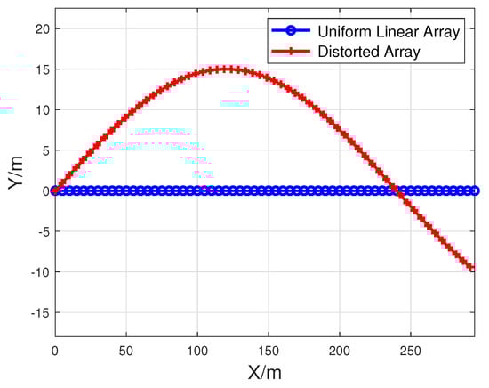
Figure 4.
Hydrophone coordinates of the actual distorted array and the hypothetical uniform linear array.
Suppose that the underwater acoustic signal radiated by a far-field target impinges on the towed array with an initial angle , and the change rate of the target angle is set to be . According to the characteristics of ship-radiated noise, a three-parameter model with Hz, Hz, and is employed to model the continuous spectrum component [50]. Besides, six sinusoidal signals with frequencies of 53 Hz, 86 Hz, 139 Hz, 382 Hz, 847 Hz, and 1451 Hz are used to model the line-spectrum components. The sound velocity in water is assumed to be 1500 m/s. The observation sequence length is set to be , and the sampling number for each observation is with a sampling rate kHz.
5.1.1. Effectiveness Evaluation of the Proposed Method
In this simulation, the effectiveness of the proposed method is investigated in detail. The SNR of all the line-spectrum components is set to be 4 dB. Figure 5a shows the acquired beam power pattern based on the hypothetical uniform linear array. Due to the time-delay mismatch in the distorted towed array, the main beam is split into two peaks, and the maximal peak is located at , which deviates from the actual target direction . Six line-spectrum components are detected from the power spectrum of the obtained pre-enhanced signal. Figure 5b presents the estimates of the time-delay difference between the first 2 hydrophones for 50 frames of observation. Figure 5c shows the estimates for the inter-hydrophone time-delay difference of the distorted towed array at the 17th observation. As seen from Figure 5b,c, the time-delay difference estimates are fluctuated around the truths for all methods except the CBF method. Moreover, the estimates in the proposed method exhibit a smaller fluctuation and are closer to the actual values, compared to those in other three methods. This is because the proposed method establishes a data-driven HMM with robustness to phase difference ambiguity by fully exploiting the underlying property of slowly changing time-delay difference over time. Thus, it is able to estimate the time-delay difference utilizing the phase difference measurements of all detected line-spectrum components from multiple frames of observation.
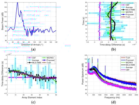
Figure 5.
Performance comparisons. (a) Beam power pattern based on the hypothetical uniform linear array. (b) The estimates of the time-delay difference between the first two hydrophones for 50 frames of observation. (c) The estimates for inter-hydrophone time-delay difference of the distorted towed array at the 17th observation. (d) The average for the power spectrum of the enhanced signal in 50 frames of observation.
Figure 5d shows the average for the power spectrum of the 50 frames of enhanced signal. It can be seen that the power spectrum of the proposed method outperforms those of its counterparts in terms of fidelity, especially for the high-frequency parts of the power spectrum. Moreover, the power spectrum of the proposed method agrees well with that acquired when the accurate hydrophone coordinates are known. To quantify the signal enhancement performance, the amplitude errors between the line-spectrum components in the power spectrum for the considered five methods and those in the power spectrum for a known array shape are listed in Table 2. It is observed that the improvement by using the proposed method is evident, and the amplitude errors of line-spectrum components in the proposed method are generally less than 0.1 dB.
Table 2.
Amplitude errors of line-spectrum components.
5.1.2. Performance Comparison versus the SNR of the Line-Spectrum Component
The effectiveness of the proposed method has been verified in the previous simulation. In this simulation, we analyze the impact of SNR of the line-spectrum component on the time-delay difference estimation accuracy of the proposed method. The estimation accuracy of time-delay difference is evaluated in terms of the root mean square error (RMSE) defined as
where denotes the estimate for time-delay difference between the and hydrophones at frame t of the run, represents the actual time-delay difference between the and hydrophones at frame t, stands for the number of Monte Carlo runs and is set to be 200 in this simulation, respectively.
In this simulation, the SNR of the line-spectrum component varies over the interval [−15, 25] dB. Other parameters are the same as those in the preceding simulation. Figure 6 shows the RMSEs of time-delay difference estimates versus the SNR of line-spectrum component for different methods. It is noted that the RMSEs of the proposed method, WORKS method, WLS-HMM method, and average method decrease as the SNR increases for SNR dB. However, the RMSE of the CBF method is almost independent of SNR and fixed at a constant. The incorrect assumption of hydrophone coordinates is the main reason resulting in time-delay difference estimation errors in this scenario. Additionally, note that the RMSEs of the proposed method are much smaller than those of its counterparts throughout the SNR interval. This is to be expected, since the proposed method extends the phase difference measurements available for time-delay difference estimation from that of low-frequency line-spectrum components in a single frame of observation to that of all detected line-spectrum components in multiple frames of observation.
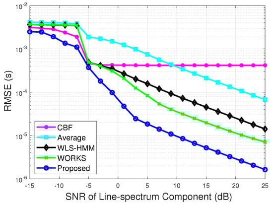
Figure 6.
RMSE of time-delay difference estimation versus SNR of the line-spectrum component.
5.2. Experimental Results of Real Sea Trial Data
In this subsection, the real data collected at sea are employed to verify the effectiveness of the proposed method. Figure 7 shows the diagram of the sea trial conducted in the South China Sea. As indicated in Figure 7, the depths of the acoustic source, the receiving hydrophone array and the seafloor are 25 m, 50 m, and 105 m, respectively. A signal is transmitted from the power amplifier (acoustic source) below the anchored transmitting ship. The power spectrum of the transmitted signal consists of continuous spectrum component and eight line-spectrum components with frequencies of 36 Hz, 97 Hz, 157 Hz, 310 Hz, 847 Hz, 1500 Hz, 3000 Hz, and 5000 Hz. The spectrum level of the continuous spectrum component is 130 dB at 1 kHz, and the powers of the line-spectrum components are 15 dB higher than their nearby continuous spectrum. The sound speed profile acquired in the sea trial area shows a weak negative gradient. The towing ship runs according to the pre-designed route with a speed of 6 knots. The distance between the acoustic source and the receiving array is about 12 km. The data are collected from a towed array comprising 60 hydrophones uniformly spaced at 6.0 m. Other parameters are the same as those in Figure 5.
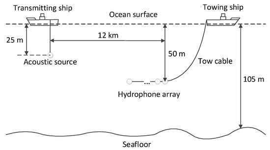
Figure 7.
Schematic diagram of the sea trial.
Figure 8a presents the direction time record during a turn of the towing ship. It is observed that the towing ship starts the turn at the time of 300 s and ends the turn at the time of 1250 s. Without loss of generality, we select 120 s of data starting from the time of 1000 s as an example to verify the effectiveness of the proposed method. Five line-spectrum components with frequencies of 36 Hz, 97 Hz, 157 Hz, 310 Hz, and 3000 Hz are detected from the pre-enhanced signal based on the hypothetical uniform linear array. Figure 8b shows the estimates of the time-delay difference between the first two hydrophones for 120 frames of observation. Figure 8c presents the estimates for the inter-hydrophone time-delay difference of the towed array at the 67th observation. As seen from Figure 8b,c, whether in time dimension or space dimension, the time-delay difference estimates in the proposed method exhibit a smaller fluctuation compared to those in other three methods.
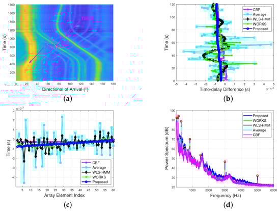
Figure 8.
Performance comparisons. (a) Direction time record during a turn of the towing ship. (b) The estimates of the time-delay difference between the first two hydrophones for all the observations. (c) The estimates for inter-hydrophone time-delay difference of the towed array at the 67th observation. (d) The average for the power spectrum of the enhanced signal in 120 frames of observation.
Figure 8d presents the average for the power spectrum of the enhanced signal in 120 frames of observation. To quantify the signal enhancement performance, the amplitude gains between the line-spectrum components in the power spectrum for the considered four methods and those in the power spectrum based on the hypothetical uniform linear array are listed in Table 3. Note that the improvement by using the proposed method is evident, particularly for the line-spectrum components with frequencies larger than 100 Hz. The time-frequency spectrum of the enhanced signal for different methods are presented in Figure 9a–e. It is observed that the line-spectrum components in the time-frequency spectrum of the proposed method have higher amplitudes than those in the time-frequency spectrum of other four methods. It is consistent with the results shown in Figure 8d and Table 3.
Table 3.
Amplitude gains of line-spectrum components.
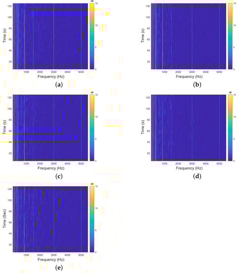
Figure 9.
Time-frequency spectrum after frequency domain equalization. (a) Proposed method. (b) WORKS method. (c) WLS-HMM method. (d) Average method. (e) CBF method.
6. Conclusions
In this paper, we proposed a time-frequency joint time-delay difference estimation method for signal enhancement in the distorted towed hydrophone array. The proposed method fully exploits the underlying property of slowly changing time-delay difference over time by modeling the change of time-delay difference as a first-order hidden Markov process. Furthermore, a data-driven HMM with robustness to phase difference ambiguity is established in the proposed method to estimate the time-delay difference. Thus, the phase difference measurements available for time-delay difference estimation are extended from that of low-frequency line-spectrum components in a single frame to that of all detected line-spectrum components in multiple frames. Since the phase difference measurements in both time and frequency dimensions are exploited jointly, the proposed method has the capability of acquiring enhanced time-delay difference estimates even in the low SNR case. Simulation results show that the signal enhancement performance of the proposed method with a distorted array is close to that of the existing approach with a known array shape, even if the SNR of all the line-spectrum components is as low as 4 dB. At-sea experimental results prove that, even though the signal of interest is contaminated by towed platform noise and real ocean ambient noise, the proposed method still achieves a better signal enhancement performance compared to these existing state-of-the-art approaches.
Author Contributions
Conceptualization, C.Z., S.F. and X.L.; methodology, C.Z., S.F. and Q.W.; software, C.Z. and Q.W.; investigation, C.Z., S.F. and L.A.; writing—original draft preparation, C.Z., Q.W. and L.A.; writing—review and editing, C.Z. and Q.W.; supervision, C.Z., S.F.; funding acquisition, S.F., H.C. and X.L. All authors have read and agreed to the published version of the manuscript.
Funding
This work was supported in part by the National Natural Science Funds of China under Grant Nos. 91938203 11874109 and 12174053, in part by the Fundamental Research Funds for the Central Universities under Grant No. 2242021k30019, in part by Science and Technology on Sonar Laboratory under Grant No. 6142109180202, and in part by National Defense Basis Scientific Research program of China under Grant No. JCKY2019110C143.
Institutional Review Board Statement
Not applicable.
Informed Consent Statement
Not applicable.
Data Availability Statement
The data presented in this paper are available after contacting the corresponding author.
Acknowledgments
The authors would like to thank the anonymous reviewers for their careful reading and valuable comments.
Conflicts of Interest
The authors declare no conflict of interest.
Appendix A
The steps of the Viterbi algorithm are presented as follows:
- Step (1)
- Initialization. Let
- Step (2)
- Recursion. For , do
- Step (3)
- Termination.
- Step (4)
- Optimal path (state sequence) backtracking. For , do
References
- Van Trees, H.L. Optimum Array Processing: Part IV of Detection, Estimation, and Modulation Theory; John Wiley & Sons: Hoboken, NJ, USA, 2004. [Google Scholar]
- Liu, W.; Weiss, S. Wideband Beamforming: Concepts and Techniques; John Wiley & Sons: Hoboken, NJ, USA, 2010. [Google Scholar]
- Wu, Q.; Zhang, H.; Lai, Z.; Xu, Y.; Yao, S.; Tao, J. An enhanced data-driven array shape estimation method using passive underwater acoustic data. Remote Sens. 2021, 13, 1773. [Google Scholar] [CrossRef]
- Wang, X.; Liu, A.; Zhang, Y.; Xue, F. Underwater acoustic target recognition: A combination of multi-dimensional fusion features and modified deep neural network. Remote Sens. 2019, 11, 1888. [Google Scholar] [CrossRef]
- Luo, X.; Shen, Z. A space-frequency joint detection and tracking method for line-spectrum components of underwater acoustic signals. Appl. Acoust. 2021, 172, 107609–107620. [Google Scholar] [CrossRef]
- Wu, Q.; Xu, P.; Li, T.; Fang, S. Feature enhancement technique with distorted towed array in the underwater radiated noise. In Proceedings of the INTER-NOISE and NOISE-CON Congress and Conference Proceedings, Hong Kong, China, 27–30 August 2017. [Google Scholar]
- Zhu, C.; Seri, S.G.; Mohebbi-Kalkhoran, H.; Ratilal, P. Long-range automatic detection, acoustic signature characterization and bearing-time estimation of multiple ships with coherent hydrophone array. Remote Sens. 2020, 12, 3731. [Google Scholar] [CrossRef]
- Hinich, M.J.; Rule, W. Bearing estimation using a large towed array. J. Acoust. Soc. Am. 1975, 58, 1023–1029. [Google Scholar] [CrossRef]
- Zheng, Z.; Yang, T.; Gerstoft, P.; Pan, X. Joint towed array shape and direction of arrivals estimation using sparse bayesian learning during maneuvering. J. Acoust. Soc. Am. 2020, 147, 1738–1751. [Google Scholar] [CrossRef] [PubMed]
- Lemon, G.S. Towed-array history, 1917–2003. IEEE J. Ocean. Eng. 2004, 29, 365–373. [Google Scholar] [CrossRef]
- Odom, J.L.; Krolik, J.L. Passive towed array shape estimation using heading and acoustic data. IEEE J. Ocean. Eng. 2015, 40, 465–474. [Google Scholar] [CrossRef]
- Hodgkiss, W. The effects of array shape perturbation on beamforming and passive ranging. IEEE J. Ocean. Eng. 1983, 8, 120–130. [Google Scholar] [CrossRef]
- Bouvet, M. Beamforming of a distorted line array in the presence of uncertainties on the sensor positions. J. Acoust. Soc. Am. 1987, 81, 1833–1840. [Google Scholar] [CrossRef]
- Felisberto, P.; Jesus, S.M. Towed-array beamforming during ship’s manoeuvring. IEE Proc. Radar Sonar Navig. 1996, 143, 210. [Google Scholar] [CrossRef]
- Gerstoft, P.; Hodgkiss, W.S.; Kuperman, W.A.; Song, H.; Siderius, M.; Nielsen, P.L. Adaptive beamforming of a towed array during a turn. IEEE J. Ocean. Eng. 2003, 28, 44–54. [Google Scholar] [CrossRef]
- Owsley, N. Shape estimation for a flexible underwater cable. IEEE Eascon 1981, 14, 16–19. [Google Scholar]
- van Ballegooijen, E.; van Mierlo, G.; van Schooneveld, C.; van der Zalm, P.; Parsons, A.; Field, N. Measurement of towed array position, shape, and attitude. IEEE J. Ocean. Eng. 1989, 14, 375–383. [Google Scholar] [CrossRef]
- Lu, F.; Milios, E.; Stergiopoulos, S.; Dhanantwari, A. New towed-array shape-estimation scheme for real-time sonar systems. IEEE J. Ocean. Eng. 2003, 28, 552–563. [Google Scholar] [CrossRef]
- Knapp, C.; Carter, G. The generalized correlation method for estimation of time delay. IEEE Trans. Acoust. Speech Signal Process. 1976, 24, 320–327. [Google Scholar] [CrossRef]
- Ferguson, B.G. Improved time-delay estimates of underwater acoustic signals using beamforming and prefiltering techniques. IEEE J. Ocean. Eng. 1989, 14, 238–244. [Google Scholar] [CrossRef]
- Fillinger, L.; Sutin, A.; Sedunov, A. Acoustic ship signature measurements by cross-correlation method. J. Acoust. Soc. Am. 2010, 129, 774–778. [Google Scholar] [CrossRef]
- Guo, W.; Piao, S.; Guo, J.; Lei, Y.; Iqbal, K. Passive detection of ship-radiated acoustic signal using coherent integration of cross-power spectrum with doppler and time delay compensations. Sensors 2020, 20, 1767. [Google Scholar] [CrossRef]
- Urick, R.J. Principles of Underwater Sound, 3rd ed.; McGraw-Hill Book Company: New York, NY, USA, 1983. [Google Scholar]
- Ross, D. Mechanics of Underwater Noise; Elsevier: Amsterdam, The Netherlands, 2013. [Google Scholar]
- Abraham, D.A. Underwater Acoustic Signal Processing: Modeling, Detection, and Estimation; Springer: Berlin/Heidelberg, Germany, 2019. [Google Scholar]
- Cavina, N.; Cesare, M.D.; Ravaglioli, V.; Ponti, F.; Covassin, F. Full load performance optimization based on turbocharger speed evaluation via acoustic sensing. In Internal Combustion Engine Division Fall Technical Conference; American Society of Mechanical Engineers: New York, NY, USA, 2014; Volume 46179, p. V002T05A006. [Google Scholar]
- Ravaglioli, V.; Cavina, N.; Cerofolini, A.; Corti, E.; Moro, D.; Ponti, F. Automotive turbochargers power estimation based on speed fluctuation analysis. Energy Procedia 2015, 82, 103–110. [Google Scholar] [CrossRef][Green Version]
- Gagliardi, G.; Tedesco, F.; Casavola, A. An adaptive frequency-locked-loop approach for the turbocharger rotational speed estimation via acoustic measurements. IEEE Trans. Control. Syst. Technol. 2020. [Google Scholar] [CrossRef]
- Moro, D.; Corti, E.; Cesare, M.D.; Serra, G. Upgrade of a Turbocharger Speed Measurement Algorithm Based on Acoustic Emission; SAE Technical Paper: Warrendale, PA, USA, 2009. [Google Scholar]
- So, H.C. Time-delay estimation for sinusoidal signals. IEE Proc. Radar Sonar Navig. 2002, 148, 318–324. [Google Scholar] [CrossRef]
- Piersol, A.G. Time delay estimation using phase data. IEEE Trans. Acoust. Speech Signal Process. 1981, 29, 471–477. [Google Scholar] [CrossRef]
- Xiao, L.; Xia, X.-G.; Wang, Y.-P. Exact and robust reconstructions of integer vectors based on multidimensional Chinese remainder theorem (MD-CRT). IEEE Trans. Signal Process. 2020, 68, 5349–5364. [Google Scholar] [CrossRef]
- Goldreich, O.; Ron, D. Chinese remaindering with errors. IEEE Trans. Inf. Theory 2000, 46, 1330–1338. [Google Scholar] [CrossRef]
- Xia, X.-G.; Wang, G. Phase unwrapping and a robust Chinese remainder theorem. IEEE Signal Process. Lett. 2007, 14, 247–250. [Google Scholar] [CrossRef]
- Li, X.; Xia, X.-G. A fast robust Chinese remainder theorem based phase unwrapping algorithm. IEEE Signal Process. Lett. 2008, 15, 665–668. [Google Scholar] [CrossRef]
- Wang, W.; Li, X.; Wang, W.; Xia, X.-G. Maximum likelihood estimation based robust Chinese remainder theorem for real numbers and its fast algorithm. IEEE Trans. Signal Process. 2015, 63, 3317–3331. [Google Scholar] [CrossRef]
- Li, X.; Huang, T.-Z.; Liao, Q.; Xia, X.-G. Optimal estimates of two common remainders for a robust generalized Chinese remainder theorem. IEEE Trans. Signal Process. 2019, 67, 1824–1837. [Google Scholar] [CrossRef]
- McKilliam, R.G.; Quinn, B.G.; Clarkson, I.V.L.; Moran, B. Frequency estimation by phase unwrapping. IEEE Trans. Signal Process. 2010, 58, 2953–2963. [Google Scholar] [CrossRef]
- Xu, Z.; Lu, T.; Huang, B. Fast frequency estimation algorithm by least squares phase unwrapping. IEEE Signal Process. Lett. 2016, 23, 776–779. [Google Scholar] [CrossRef]
- Zhu, C.; Fang, S.; Wu, Q.; An, L.; Luo, X. Robust wideband DOA estimation based on element-space data reconstruction in a multi-source environment. IEEE Access 2021, 9, 43522–43539. [Google Scholar] [CrossRef]
- Yang, T. Deconvolved conventional beamforming for a horizontal line array. IEEE J. Ocean. Eng. 2017, 43, 160–172. [Google Scholar] [CrossRef]
- Kay, S.M. Fundamentals of Statistical Signal Processing, Volume I: Estimation Theory; Prentice Hall PTR: Lebanon, IN, USA, 1993. [Google Scholar]
- Quinn, B.G. Estimating the mode of a phase distribution. In Proceedings of the Conference on Signals, Systems & Computers, Pacific Grove, CA, USA, 16–18 December 2007. [Google Scholar]
- Rabiner, L.R. A tutorial on hidden Markov models and selected applications in speech recognition. Proc. IEEE 1989, 77, 257–286. [Google Scholar] [CrossRef]
- García, M.A.; Moutahir, H.; Casady, G.M.; Bautista, S.; Rodríguez, F. Using hidden Markov models for land surface phenology: An evaluation across a range of land cover types in southeast Spain. Remote Sens. 2019, 11, 507. [Google Scholar] [CrossRef]
- Asadi, N.; Mirzaei, A.; Haghshenas, E. Multiple observations HMM learning by aggregating ensemble models. IEEE Trans. Signal Process. 2013, 61, 5767–5776. [Google Scholar] [CrossRef]
- Scherhäufl, M.; Hammer, F.; Pichler-Scheder, M.; Kastl, C.; Stelzer, A. Radar distance measurement with Viterbi algorithm to resolve phase ambiguity. IEEE Trans. Microw. Theory Tech. 2020, 68, 3784–3793. [Google Scholar] [CrossRef]
- Djukanović, S.; Popović-Bugarin, V. Efficient and accurate detection and frequency estimation of multiple sinusoids. IEEE Access 2018, 7, 1118–1125. [Google Scholar] [CrossRef]
- Li, Q. Digital Sonar Design in Underwater Acoustics: Principles and Applications; Springer Science & Business Media: Berlin/Heidelberg, Germany, 2012. [Google Scholar]
- Wales, S.C.; Heitmeyer, R.M. An ensemble source spectra model for merchant ship-radiated noise. J. Acoust. Soc. Am. 2002, 111, 1211–1231. [Google Scholar] [CrossRef]


Publisher’s Note: MDPI stays neutral with regard to jurisdictional claims in published maps and institutional affiliations. |
© 2021 by the authors. Licensee MDPI, Basel, Switzerland. This article is an open access article distributed under the terms and conditions of the Creative Commons Attribution (CC BY) license (https://creativecommons.org/licenses/by/4.0/).