Generation of High-Precision Ground Penetrating Radar Images Using Improved Least Square Generative Adversarial Networks

Abstract

Deep learning models have achieved success in image recognition and have shown great potential for interpretation of ground penetrating radar (GPR) data. However, training reliable deep learning models requires massive labeled data, which are usually not easy to obtain due to the high costs of data acquisition and field validation. This paper proposes an improved least square generative adversarial networks (LSGAN) model which employs the loss functions of LSGAN and convolutional neural networks (CNN) to generate GPR images. This model can generate high-precision GPR data to address the scarcity of labelled GPR data. We evaluate the proposed model using Frechet Inception Distance (FID) evaluation index and compare it with other existing GAN models and find it outperforms the other two models on a lower FID score. In addition, the adaptability of the LSGAN-generated images for GPR data augmentation is investigated by YOLOv4 model, which is employed to detect rebars in field GPR images. It is verified that inclusion of LSGAN-generated images in the training GPR dataset can increase the target diversity and improve the detection precision by 10%, compared with the model trained on the dataset containing 500 field GPR images.

1. Introduction

Ground penetrating radar (GPR) is a popular geophysical technique and has been widely applied to near-surface investigation [1,2], archaeological prospection [3,4], hydrological investigation [5], lunar exploration [6], and civil engineering [7]. In tunnel detection, GPR is used to detect voids, seepage, and rebar defects [8,9]. In bridge field, GPR is commonly used to measure reinforcement position, concrete thickness, and reinforcement corrosion degree [10,11]. With the rapid increase of detection requirements in civil engineering, GPR has been become a regular method for inspecting reinforced bars (rebars) in concrete, locating subsurface pipelines, structural performance evaluation, etc. [12]. A single scatterer, such as a landmine, rebar, or pipeline, reflects a hyperbolic signature in a recorded GPR B-scan profile [13], which can be used to locate the buried objects from GPR images [14]. However, even for an experienced practitioner, interpretation of GPR data is extremely time- and labor-consuming due to complex field conditions and huge data volumes. For example, field data detected by a car-mounted GPR system in a day would take one week or even longer to be comprehensively interpreted [15]. Therefore, the low efficiency of manual interpretation is a major factor that limits the fast decision-making for maintenance and rehabilitation [16,17].

As a branch of machine learning, neural networks have been developed over 40 years, and one of the hotspots is the application of convolutional neural networks (CNN) [18]. CNN with multiple hidden layers have shown strong ability in recognition of computer vision features and present high robustness in detection task, which has shown their potential in GPR scenarios [19]. In this context, a series of network architectures, such as Faster region-based CNN (Faster R-CNN) and Single Shot MultiBox Detector (SSD), have been applied to the GPR image recognition tasks [20,21,22]. Pham et al. [23] applied a pre-trained Faster R-CNN model to GPR image identification, proving that deep learning-based algorithms make an improvement compared to classical computer vision methods. Giannakis et al. [24] combined neural networks and a random forest regression algorithm to recognize GPR images. Nonetheless, training a deep learning model requires massive GPR data with labels of subsurface targets. Due to the high costs of data acquisition and field validation, massive GPR data for CNNs are not readily available.

Up to now, a challenging aspect impeding the extension of deep learning methods is the limited amount of GPR data with labels for training. To solve this issue, simulation is an available way to add the amount of training GPR data. GprMax, an open-source software based on finite-difference time domain (FDTD) method, has been widely used for simulating GPR data [25,26]. However, the field radar profiles are more complicated than simulated radar profiles due to the complex dielectric distributions in real measurement scenarios, which are hardly modelled. With the development of deep learning techniques, generative adversarial networks (GAN) present a new way to generate GPR images [27,28,29]. Nonetheless, training GAN is still a difficult issue in practice due to the instability of the GAN’s learning process which is usually caused by the objective function [30,31]. Radford et al. [31] raised a deep convolutional generative adversarial networks (DCGAN), which improves the convergence of the GAN and the quality of generated images. Mao et al. [32] changed the objective function of GAN from cross entropy loss to least square loss and proposed a least square generative adversarial network (LSGAN), to improve the quality of the GAN-generated images and the stability of the training process. However, the GAN’s generator is prone to mode collapse during training [33]. The consequence is that the generated images could be exactly the same as the real ones, and their diversity is decreased.

This paper proposes an improved LSGAN model for generation of high-precision GPR images. As an example, generated GPR images of rebar in concrete are presented. Then the influence of the amount of generated GPR data on the hyperbolic recognition precision is investigated. Finally, the recognition performance is tested using GPR data recorded on reinforced concrete structures. The rest of this paper is organized as follows. Architecture of the improved LSGAN model is introduced in Section 2. Section 3 presents and evaluates the results produced by the LSGAN model. In the Section 4, the impact of the amount of generated data on the recognition precision of the CNN model is tested. Section 5 discusses the characteristics of our proposed algorithm. Conclusions are given in the last section.

2. Methodology

2.1. Generative Adversarial Networks (GAN)

GAN can generate artificial images by using two adversarial networks. A GAN architecture is composed of two component parts, including a generation model G and a discriminant model D (Figure 1) [34]. The G model is responsible for producing spurious data whereas the D model is in charge of distinguishing the authenticity of the produced data. Competition between D and G makes the two models equal to optimize the training process until reaching a balanced state. The generated image of the generator G is rated by a discriminator D which distinguishes between the field data $p_{data}\left(x\right)$ and the generated data $p_z\left(z\right)$. The generator G will confuse the discriminator D to judge whether the generated data is true or not. The loss function in GAN is defined as follows

$$\underset{G}{\min } \underset{D}{\max }V\left(D,G\right)=E_{x~P_{data}}\left[LogD\left(x\right)\right]+E_{z~P_z}\left[log\left(1-D\left(G\left(z\right)\right)\right)\right]$$

(1)

where G(z) is a sample image generated by a random matrix, x is a field sample image, $E_{x~P_{data}}$ is the expected value over all field instances, and $E_{z~P_z}$ is the expected value over all the fake instances.

The convergence direction of the network is achieved by $\underset{G}{\min } \underset{D}{\max }V\left(D,G\right)$. The loss function in Equation (1) can be divided into two parts which correspond to the discriminative model and the generative model, respectively.

$$LOS{S}_{\left(D\right)}=-\left(\log \left(D\left(x\right)\right)+\log \left(1-D\left(G\left(z\right)\right)\right)\right)$$

(2)

$$LOS{S}_{\left(G\right)}=-\left(\log \left(D\left(G\left(z\right)\right)\right)\right)$$

(3)

However, GAN is unstable and easily results in non-convergence during the training process [29]. In addition, the instability of the GAN makes it prone to under-fitting or over-fitting [35]. Therefore, the parameters of GAN must be carefully adjusted in the training process.

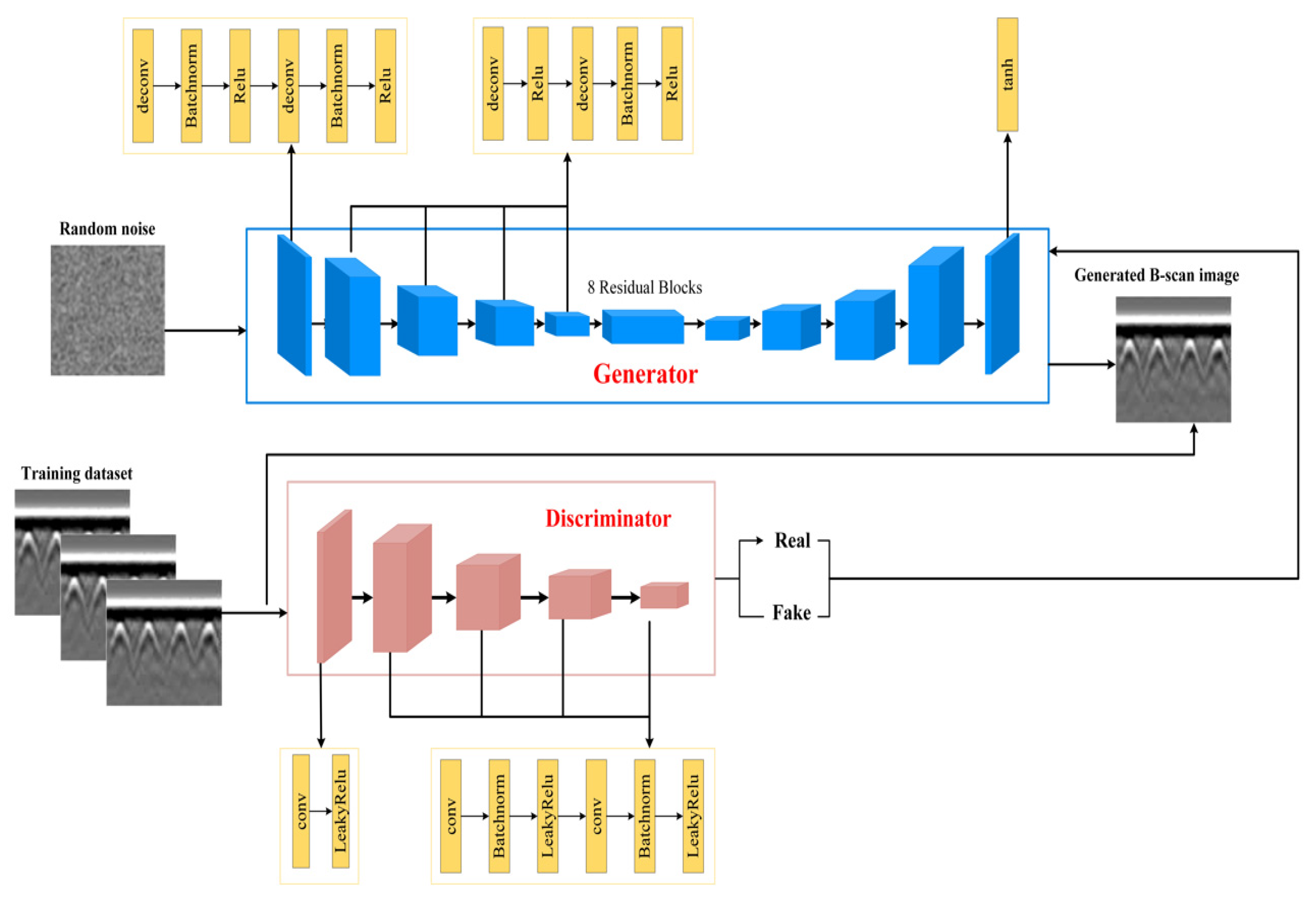
2.2. Improved Least Square Generative Adversarial Networks

LSGAN adopts the least square loss function of the discriminator and can generate images that are closer to field GPR images than the normal GANs [32]. The loss functions of the generator and discriminator of the LSGAN are respectively defined as follows:

$$\underset{D}{\min }{V}_{LSGAN}\left(\mathrm{D}\right)=\frac{1}{2}{E}_{x~P_{data}}\left[{\left(D\left(x\right)-b\right)}^2\right]+\frac{1}{2}{E}_{z~P_z}\left[{\left(D\left(G\left(z\right)\right)-a\right)}^2\right]$$

(4)

$$\underset{G}{\min }{V}_{LSGAN}\left(\mathrm{G}\right)=\frac{1}{2}{E}_{z~P_z}\left[{\left(D\left(G\left(z\right)\right)-c\right)}^2\right]$$

(5)

where a is the label of fake data, b is the label of field data, and c is the value set by G for D to determine whether the generated image is real data.

However, LSGAN models suffer from the following problems [36]:

(a)

The generator is susceptible to collapse during the training process;

(b)

The generator gradient may vanish and learn nothing;

(c)

The generated images are not diverse.

In this paper, we improve the architecture of LSGAN, as shown in Figure 2. It can smooth the gradient and improve the stability of the adversarial training, thus reducing the possibility of mode collapses in training stage and increasing the variety of generated images.

The generator’s detailed architecture is presented in

Table 1. The framework of generator model.

Type	Layer	Output Shape
ConvTranspose1	ConvTranspose2d	[1,4,4,4096]
	ReLU	[1,4,4,4096]
	ConvTranspose2d	[1,2048,8,8]
	BatchNorm2d	[1,2048,8,8]
	ReLU	[1,2048,8,8]
ConvTranspose2 (Up3)	ConvTranspose2d	[1,1024,16,16]
	BatchNorm2d	[1,1024,16,16]
	ReLU	[1,1024,16,16]
	ConvTranspose2d	[1,512,32,32]
	BatchNorm2d	[1,512,32,32]
	ReLU	[1,512,32,32]
ConvTranspose3 (Up2)	ConvTranspose2d	[1,256,64,64]
	BatchNorm2d	[1,256,64,64]
	ReLU	[1,256,64,64]
	ConvTranspose2d	[1,128,128,128]
	BatchNorm2d	[1,128,128,128]
	ReLU	[1,128,128,128]
ConvTranspose4 (Up1)	ConvTranspose2d	[1,64,256,256]
	BatchNorm2d	[1,64,256,256]
	ReLU	[1,64,256,256]
	ConvTranspose2d	[1,64,256,256]
	BatchNorm2d	[1,1,512,512]
	ReLU	[1,1,512,512]
ResNet	Residual Blocks	[1,1,512,512]
Up4	ConvTranspose2d	[1,64,256,256]
	BatchNorm2d	[1,64,256,256]
	ReLU	[1,64,256,256]
	ConvTranspose2d	[1,64,256,256]
	BatchNorm2d	[1,1,512,512]
	ReLU	[1,1,512,512]
	Tanh	[1,1,512,512]

. The purpose of the generator is to create an image from the input image based on a random noise matrix. Several up-sampling operations are set to reshape the size of input matrix (512 × 512 in this work). The design of the generator involves a transposed convolutional block to up-sample the input image. Eight transposed convolutional blocks are used in the improved LSGAN. Each block consists of a transposed convolutional layer, followed by a Batch Normalization and a Rectified Liner Unit (ReLU) activation function. In the first block, the kernel of transposed convolutional layer is 4 × 4 with a stride of one that resizes the input matrix to 4 × 4 with 4096 channels. Then the stride of transposed convolutional layer is set as two with a number of features divided by two at each block. The residual block module is used to connect with the up-sampling module. A transposed convolution with a size of 4 × 4 and a stride of two followed by Tanh is set as the last block to resize the output to be 512 × 512.

Table 2. The framework of discriminator model.

Type	Layer	Output Shape
Conv1	Conv2d	[1,32,512,512]
	LeakyReLU	[1,32,512,512]
Conv2	Conv2d	[1,64,256,256]
	BatchNorm2d	[1,64,256,256]
	LeakyReLU	[1,64,256,256]
	Conv2d	[1,128,128,128]
	BatchNorm2d	[1,128,128,128]
	LeakyReLU	[1,128,128,128]
Conv3	Conv2d	[1,256,64,64]
	BatchNorm2d	[1,256,64,64]
	LeakyReLU	[1,256,64,64]
	Conv2d	[1,512,32,32]
	BatchNorm2d	[1,512,32,32]
	LeakyReLU	[1,512,32,32]
Conv4	Conv2d	[1,1024,16,16]
	BatchNorm2d	[1,1024,16,16]
	LeakyReLU	[1,1024,16,16]
	Conv2d	[1,2048,8,8]
	BatchNorm2d	[1,2048,8,8]
	LeakyReLU	[1,2048,8,8]
Conv5	Conv2d	[1,4096,4,4]
	BatchNorm2d	[1,4096,4,4]
	LeakyReLU	[1,4096,4,4]
	Conv2d	[1,1,1,1]
	BatchNorm2d	[1,1,1,1]
	LeakyReLU	[1,1,1,1]

shows the composition of the discriminator. The input of the discriminator model is the fake and real images from the generator. During training, the discriminator compares two kinds of images, and the output is used to adjust the generator to make images resemble real ones. The LeakyReLU activation function is used to avoid mode collapse [37]. Conv1 includes a 4 × 4 convolutional block with a stride of two, followed by LeakyReLU activation. Then seven 4 × 4 convolutional blocks with a stride of two, and several features are multiplied by two at each stage.

2.3. Evaluation Index

Generally, inception score (IS) [38] and Frechet Inception Distance (FID) [39] are two widely accepted measures for evaluating the performance of GAN models [40]. The IS measure directly evaluates the generated image itself by calculating its entropy. In contrast, the FID measurement calculates the similarity between the generated images and the field images [39] and thus is superior to IS measurement [38]. In this paper, FID score is used to evaluate the results of the improved LSGAN algorithm.

The FID score presents the feature distance between the real and GAN generated images, which is also known as Frechet distance between the two multivariate Gaussians. A lower FID score means closer proximity between the two distributions, which means higher quality and greater diversity of images generated. The FID score is given by

$$d_{FID}(\mathrm{x},\mathrm{g})={\parallel {\mu }_x-{\mu }_g\parallel }^2+Tr\left[{\mathsf{\Sigma }}_x+{\mathsf{\Sigma }}_g-2{\left({\mathsf{\Sigma }}_x{\mathsf{\Sigma }}_g\right)}^{\frac{1}{2}}\right]$$

(6)

where ${\mathsf{\Sigma }}_x$ and ${\mathsf{\Sigma }}_g$ are the covariance matrix of field and generated images, Tr is the trace calculated from the sum of the elements along the main diagonal of the square matrix, and µ_x, µ_g are the dimensional activations for field images and generated images, respectively.

3. Datasets of GPR Images

3.1. Data Collection

Field GPR images were obtained in several residential buildings of two construction sites by using a commercial GPR system with a central frequency of 2 GHz (Figure 3). The GPR data were recorded by a distance-measuring odometer, and the acquisition parameters are summarized in

Table 3. Parameters for GPR data acquisition.

Parameter	Value
Central frequency	2 GHz
Trace interval	0.04 m
Time window	6 ns
Samples	512

. In order to enable the dataset to cover as much as possible of all types of rebars, GPR images were collected on the surface of concrete walls, columns, beams, and slabs. Since the dimensions of these concrete components are not the same for different buildings, the GPR survey lines have various lengths. By data processing, we set each GPR image to be of the size of 512 × 512. In total, 500 GPR images which contain 2856 rebars were collected, as shown in Figure 4. Since GPR measurements were conducted before the building decoration, we can confirm that all the near-surface hyperbolic features are generated by the concrete rebars. A single rebar reflection can be easily identified due to its hyperbolic feature, and the field GPR images that are used for training the deep learning model will be described and tested in the next section.

3.2. Data Augmentation Methods

The recognition sample library needs a large amount of GPR images to successfully train the neural network model. Though 500 images have been obtained, labeled field GPR data are still limited. In this work, the improved LSGAN is used to generate more GPR data which supply the amount of training data. In this section, the obtained field GPR images are used as the training dataset in the training of the improved LSGAN. The training process is conducted on a computer with a NVIDIA GeForce GTX 1660Ti graphics card (6 GB memory). It takes 8.5 h for 500 epochs to obtain produced weight file, which is about the same as the training time with other GANs. After obtaining the weight file, each artificial GPR image can be generated within 1 s.

Figure 5 shows the visual inspection in the improved LSGAN training process. Starting from an image of random noise, the improved LSGAN adjusts the network parameters to produce GPR images resembling the real ones. At 10 epochs, the generated image has contained some prominent features, but details are lacking. When epochs reach 100, there are subtle features which resemble the rebar reflections emerged. At 200 epochs, the generated image reveals more details and looks similar to a field GPR image. When it reaches 500 epochs, the generated image contains almost all the detailed information of the field GPR images. With the improved LSGAN, we generate 500 GPR images containing 2602 rebars to augment the training dataset.

3.3. Results of Other GANs

In addition to the improved LSGAN, other GAN models, i.e., DCGAN and LSGAN, are used to generate GPR images. Their results are compared with the images generated by the proposed improved LSGAN. As shown in Figure 6, the clarity of the images generated by DCGAN is poor, and the hyperbolic characteristics of rebar reflection are not well learned by LSGAN. In comparison, GPR images generated by the improved LSGAN reveal more details than the other two.

The calculated FID score by using PyTorch shows that the improved LSGAN model achieves a FID score of 29.6 (lower scores correspond to better GAN performance). The FID score of DCGAN and LSGAN are, respectively, 67.5 and 47.6, which are much higher than results by the improved LSGAN. It means that the improved LSGAN can extract more rebar features than the DCGAN and LSGAN from field GPR images. More importantly, the images generated by the improved LSGAN contain more rebar targets than the field GPR images, which improves the diversity of training dataset.

4. Results

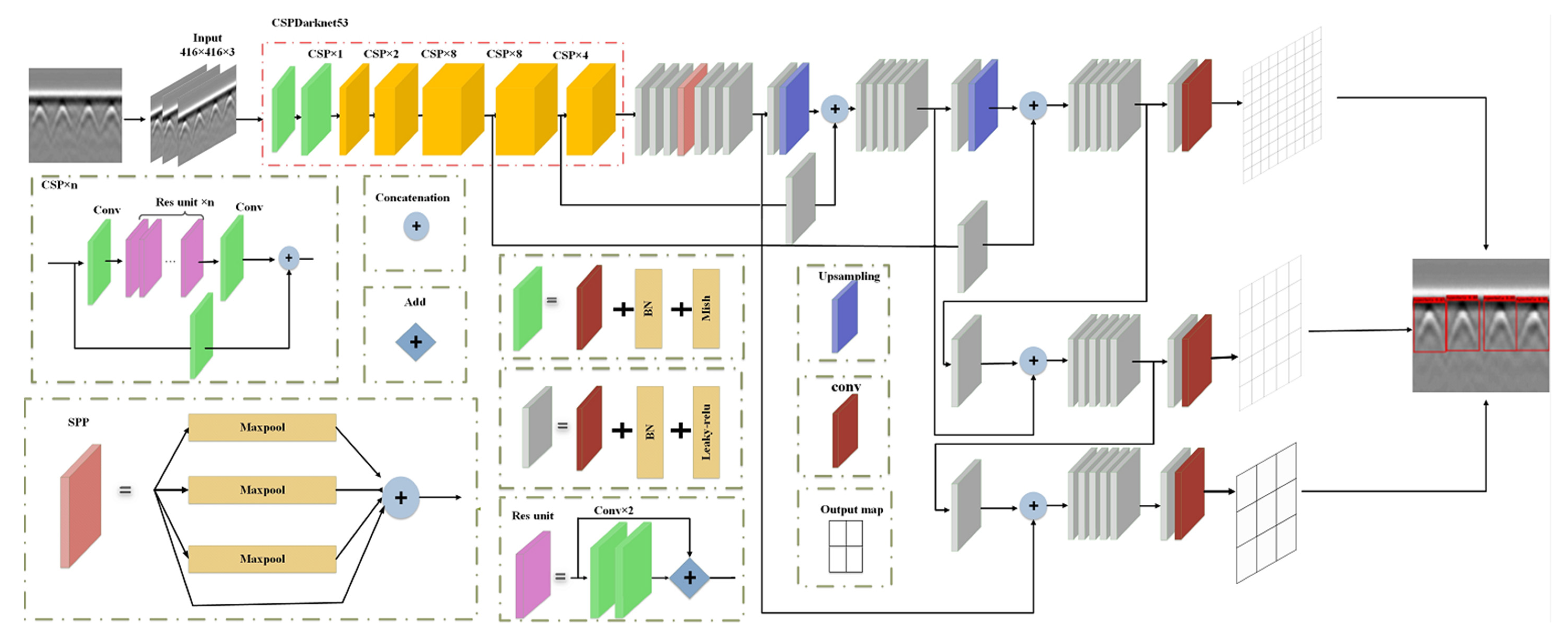
4.1. Pre-Trained YOLOv4

Since GPR data acquisition can be operated at an ultra-fast speed, both the detection accuracy and speed of a deep learning model are important in the GPR application scenarios. Therefore, we employ YOLOv4 model which improves YOLOv3’s average precision and frame per second by 10% and 12%, respectively [41], to test the value of the generated GPR images by the improved LSGAN.

The schematic diagram of YOLOv4’s network structure is shown in Figure 7. To reduce the number of required training images and iterations, transfer learning is utilized for training the Yolov4 model. In this study, the employed Yolov4 model is firstly pre-trained on the COCO dataset [42]. Then the pre-trained Yolov4 model is further trained and fine-tuned by using the acquired GPR dataset.

4.2. Testing Results

After data augmentation, the training dataset contains 500 field GPR images and 500 GAN-generated GPR images. A total of 5467 rebars are labeled manually as targets. To test the impact of generated GPR images in training dataset on the target recognition, three training datasets are created, as shown in

Table 4. Setup of the training GPR dataset.

Training Dataset	I	II	III
Field GPR image	√	×	√
Improved LSGAN image	×	√	√

√ dataset used for deep learning training. × dataset not used for deep learning training.

, and the corresponding recognition precisions are investigated. The computing facility for training YOLOv4 is the same as that used in training the improved LSGAN architecture.

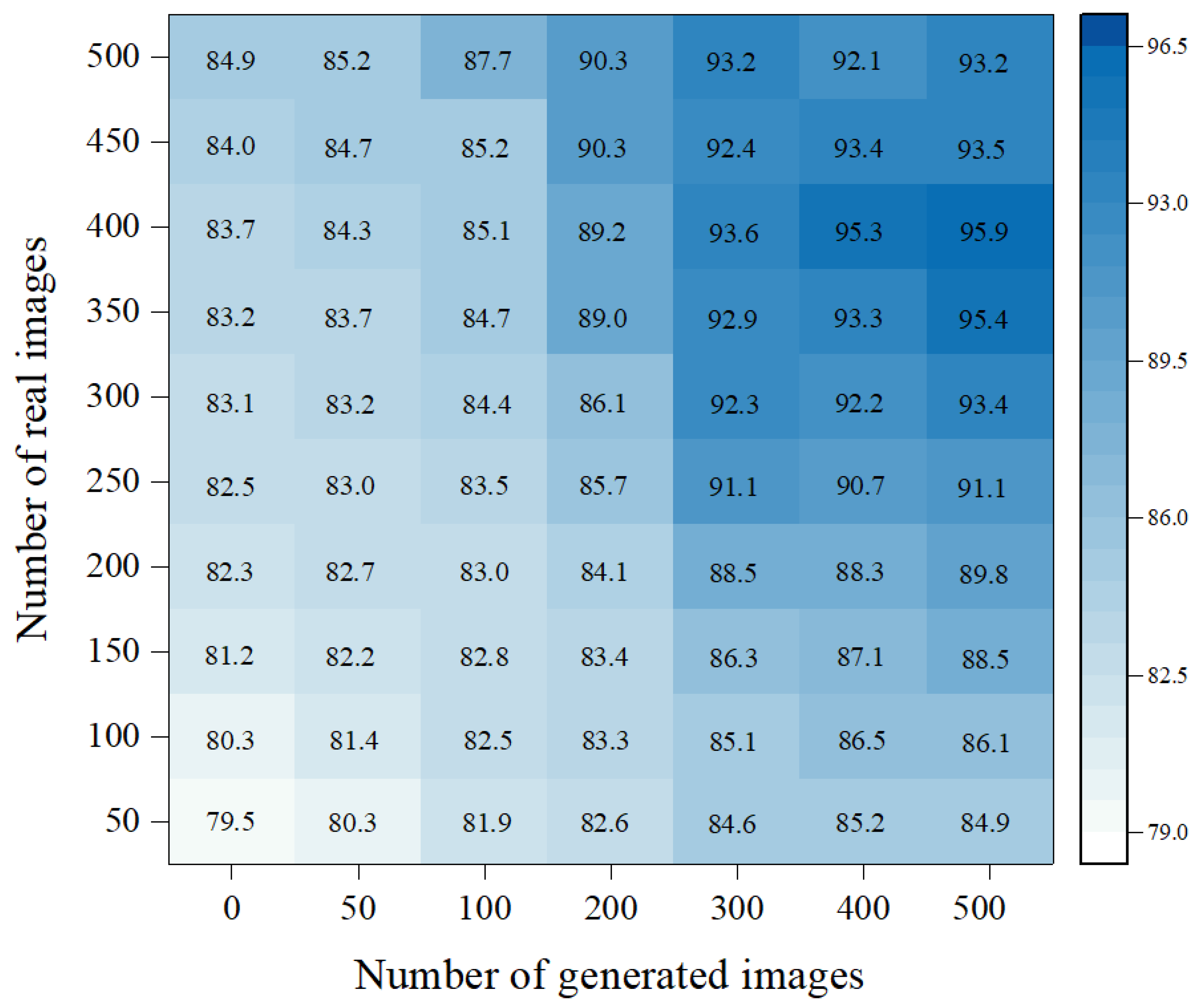
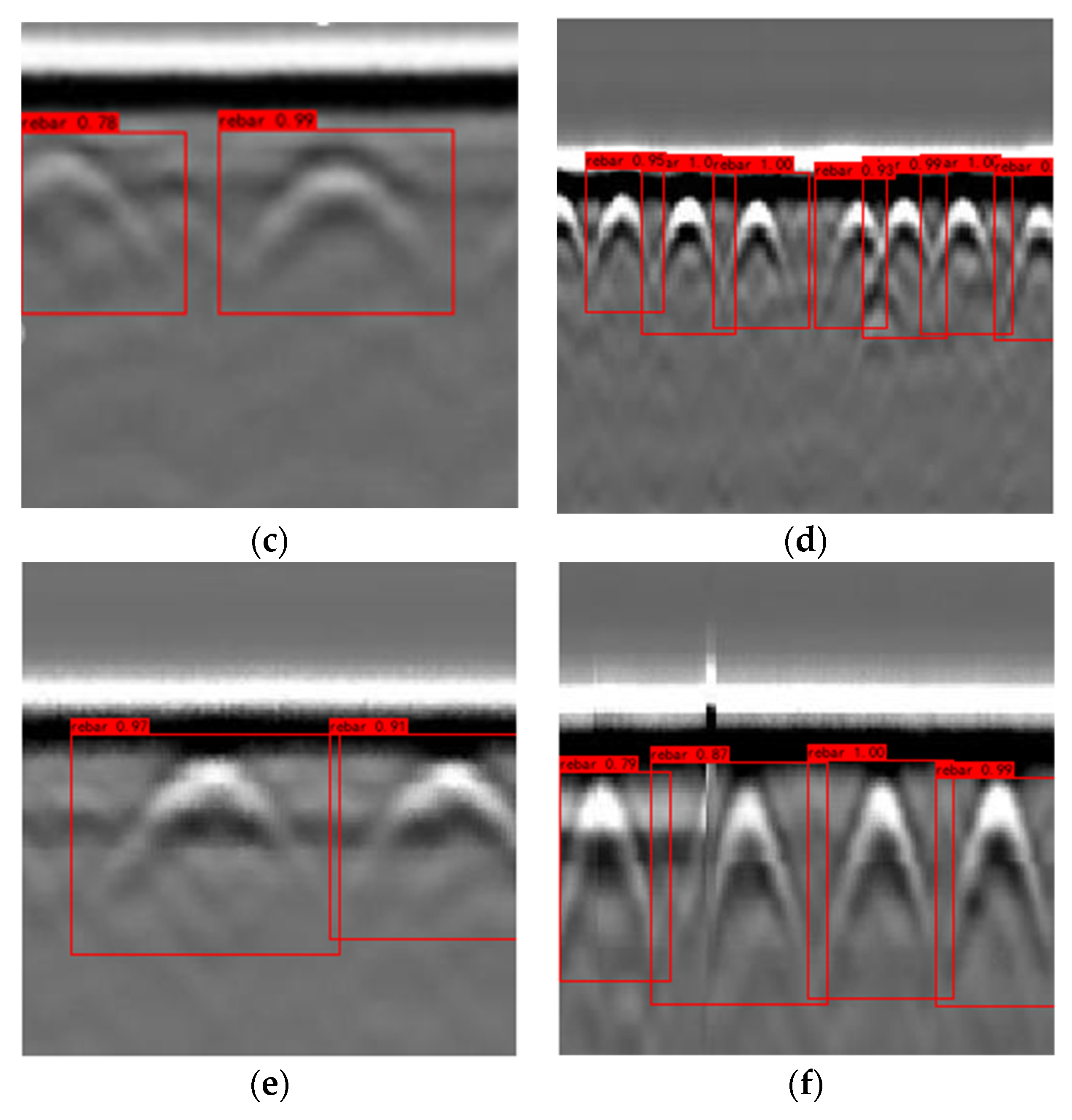
4.2.1. Training Dataset I and II

Training dataset I contains 500 field GPR images, training dataset II contains 500 generated GPR images. All the images are resized to 512 × 512 pixels. A total of 2865 rebars are labeled in dataset I, and 2602 rebars are labeled in dataset II. In each training dataset, 350 images (70%) are randomly selected for training, and the remaining 150 images (30%) are used for validation.

The YOLOv4 network is trained using the Adam optimizer with a learning rate of 0.001 and a weight decay of 0.0001, and the average training and validation losses are plotted in Figure 8. The network is improved gradually during the training process and reaches a steady state after 100 training epochs. The loss values for validation are close to those for training, indicating that no overfitting has occurred. Thus, the network is well trained and ready for recognition.

Next, we investigate the recognition precision of the trained network using 100 field GPR images that are not included in the training dataset. Classical evaluation metrics including precision (Pr), recall (Re), and F1 score (F1) are applied to evaluate the performance of the trained YOLOv4 model for rebar detection in GPR images. The Pr, Re, and F1 of the testing results of the validation images are averaged values.

$$Pr=\frac{correctly detected rebars}{all detected rebars}$$

(7)

$$Re=\frac{correctly detected rebars}{all ground-truth rebars}$$

(8)

$$F1=\frac{2\times Pr\times Re}{Pr+Re}$$

(9)

Training results of 100 iterations are then used to evaluate the performance of the trained YOLOv4 algorithm for rebar detection, as shown in Figure 9. The overall Pr, Re, and F1 scores of dataset I are 84.9%, 81.2%, and 83.1%, respectively, while those of dataset II are 84.9%, 76.4%, and 80.3%, respectively. The generated dataset image can only simulate the field GPR measurement environment with high precision but cannot be identical with field GPR images. Thus, a small number of rebars in the test field GPR dataset are not detected, resulting in low recall rate and F1 score. Nevertheless, Datasets I and II result in the same detection precision. It means that the GPR image generated by the improved LSGAN can be used to train the detection model.

4.2.2. Training Dataset III

Training dataset III contains the 500 field GPR images and a number of additional generated images. The YOLOv4 network is trained with different proportions of generated images using the same training parameters as those of the previous cases. Figure 10 shows the recognition precision. The highest precision for recognizing rebars reaches 95.9%, which is higher than the precisions using training datasets I and II.

Figure 11 shows some examples of GPR images, in which the hyperbolic reflections of rebar are identified in different scenarios. It can be seen that almost all the hyperbolic rebars in these situations are correctly identified with a high confidence, including multiple targets, closely aligned targets, overlapped targets, and blurred targets. In addition, we have further propose an automatic localization method through migration and binarization, which can accurately estimate the rebar position information [17].

5. Discussion

This paper proposes an improved LSGAN model for generation of high-precision GPR images. The loss function of LSGAN can smooth the gradient and improve the stability of the training process, thus decreasing the possibility of mode collapses and increasing the variety of generated images. Eight residual blocks and tanh function in generator are aimed to reduce the training error of deep network. Moreover, LeakyReLU activation function is applied in discriminator to improve the learning ability and also avoid mode collapse. The results show that the quality of the images produced by the proposed improved LSGAN is better than that generated by DCGAN and LSGAN at the same epochs.

In order to verify the feasibility of the generated GPR images for data augmentation, three different training datasets (dataset I to III) are used to train the YOLOv4 models and illustrate the recognition precisions. Results reveal that datasets I and II present same detection precision, but a small number of rebars in the Dataset II are not detected, resulting a low recall rate and F1 score. With the increasing of the number of improved LSGAN GPR images (dataset III), the precision of rebar recognition rises to 95.9% when 500 generated images and 400 field images are used for training. In our previous work [17], a training dataset of 3992 GPR images containing 13,026 rebars is established by another simple data augmentation method, i.e., the horizontally flipping and scaling, and the precision of rebar recognition can only reach 90.9%. In comparison, image augmentation by the improved LSGAN algorithm achieves a higher recognition precision of 95.9% by using only 900 images for training. This finding demonstrates that the GPR images generated by the improved LSGAN have abundant diversity, which can be used to train the neural network model.

6. Conclusions

In this paper, we propose an improved LSGAN for generation of GPR images to deal with the insufficient GPR images with labels for training the deep learning models with an aim of automatic subsurface target detection. Compared with other GANs, the improved LSGAN can generate GPR images of rebar with a higher precision, while ensuring the diversity of images. Furthermore, the improved LSGAN approach is employed for GPR data augmentation. It is found that the generated images can supplement the missing features in the field GPR data, increase the diversity of the dataset, and improve the recognition precision by 10%, compared with the precision of 84.9% achieved by using 500 field GPR images for training.

The future work will try to apply the improved LSGAN to generate GPR images of other underground targets, such as subsurface pipes, landmines, cavities, etc. In addition, the improved LSGAN will be trained by combining FDTD simulation and field images to make the generated images more diverse.

References

1. Liu, H.; Lu, H.; Lin, J.; Han, F.; Liu, C.; Cui, J.; Spencer, B.F. Penetration Properties of Ground Penetrating Radar Waves Through Rebar Grids. IEEE Geosci. Remote Sens. Lett. 2020, 18, 1199–1203. [Google Scholar] [CrossRef]
2. Wang, H.; Liu, H.; Cui, J.; Hu, X.; Sato, M. Velocity analysis of CMP gathers acquired by an array GPR system “Yakumo”: Results from field application to tsunami deposits. Explor. Geophys. 2017, 49, 669–674. [Google Scholar] [CrossRef]
3. Bigman, D.P.; Lanzarone, P.M. Investigating Construction History, Labour Investment and Social Change at Ocmulgee National Monument’s Mound A, Georgia, USA, Using Ground-penetrating Radar. Archaeol. Prospect. 2014, 21, 213–224. [Google Scholar] [CrossRef]
4. Bigman, D.P.; Day, D.J.; Balco, W.M. The roles of macro- and micro-scale geophysical investigations to guide and monitor excavations at a Middle Woodland site in northern Georgia, USA. Archaeol. Prospect. 2021, 10. [Google Scholar] [CrossRef]
5. Liu, H.; Xie, X.; Cui, J.; Takahashi, K.; Sato, M. Groundwater level monitoring for hydraulic characterization of an unconfined aquifer by common mid-point measurements using GPR. J. Environ. Eng. Geophys. 2014, 19, 259–268. [Google Scholar] [CrossRef]
6. Xiao, Y.; Su, Y.; Dai, S.; Feng, J.; Xing, S.; Ding, C.; Li, C. Ground experiments of Chang’e-5 lunar regolith penetrating radar. Adv. Space Res. 2019, 63, 3404–3419. [Google Scholar] [CrossRef]
7. Kravitz, B.; Mooney, M.; Karlovsek, J.; Danielson, I.; Hedayat, A. Void detection in two-component annulus grout behind a pre-cast segmental tunnel liner using Ground Penetrating Radar. Tunn. Undergr. Space Technol. 2019, 83, 381–392. [Google Scholar] [CrossRef]
8. Qin, H.; Zhang, D.; Tang, Y.; Wang, Y. Automation in Construction Automatic recognition of tunnel lining elements from GPR images using deep convolutional networks with data augmentation. Autom. Constr. 2021, 130, 103830. [Google Scholar] [CrossRef]
9. Ye, Z.; Zhang, C.; Ye, Y.; Zhu, W. Application of transient electromagnetic radar in quality evaluation of tunnel composite lining. Constr. Build. Mater. 2020, 240, 117958. [Google Scholar] [CrossRef]
10. Dinh, K.; Gucunski, N.; Duong, T.H. Automation in Construction An algorithm for automatic localization and detection of rebars from GPR data of concrete bridge decks. Autom. Constr. 2018, 89, 292–298. [Google Scholar] [CrossRef]
11. Kaur, P.; Dana, K.J.; Romero, F.A.; Gucunski, N. Automated GPR Rebar Analysis for Robotic Bridge Deck Evaluation. IEEE Trans. Cybern. 2016, 46, 2265–2276. [Google Scholar] [CrossRef] [PubMed]
12. Im, H.-C. Measurements of dielectric constants of soil to develop a landslide prediction system. Smart Struct. Syst. 2011, 7, 319–328. [Google Scholar] [CrossRef]
13. Zhang, J.; Zhang, C.; Lu, Y.; Zheng, T.; Dong, Z.; Tian, Y.; Jia, Y. In-situ recognition of moisture damage in bridge deck asphalt pavement with time-frequency features of GPR signal. Constr. Build. Mater. 2020, 244, 118295. [Google Scholar] [CrossRef]
14. Zhang, W.Y.; Hao, T.; Chang, Y.; Zhao, Y.H. Time-frequency analysis of enhanced GPR detection of RF tagged buried plastic pipes. NDT E Int. 2017, 92, 88–96. [Google Scholar] [CrossRef]
15. Liu, H.; Shi, Z.; Li, J.; Liu, C.; Meng, X.; Du, Y.; Chen, J. Detection of road cavities in urban cities by 3D ground-penetrating radar. Geophysics 2021, 86, WA25–WA33. [Google Scholar] [CrossRef]
16. Dou, Q.; Wei, L.; Magee, D.R.; Cohn, A.G. Real-Time Hyperbola Recognition and Fitting in GPR Data. IEEE Trans. Geosci. Remote Sens. 2017, 55, 51–62. [Google Scholar] [CrossRef] [Green Version]
17. Liu, H.; Lin, C.; Cui, J.; Fan, L.; Xie, X.; Spencer, B.F. Detection and localization of rebar in concrete by deep learning using ground penetrating radar. Autom. Constr. 2020, 118, 103279. [Google Scholar] [CrossRef]
18. Liu, H.; Wu, K.; Xu, H.; Xu, Y. Lithology Classification Using TASI Thermal Infrared Hyperspectral Data with Convolutional Neural Networks. Remote Sens. 2021, 13, 3117. [Google Scholar] [CrossRef]
19. Besaw, L.E.; Stimac, P.J. Deep convolutional neural networks for classifying GPR B-scans. In Detection and Sensing of Mines, Explosive Objects, and Obscured Targets XX.; International Society for Optics and Photonics: Washington, DC, USA, 2015; Volume 9454, p. 945413. [Google Scholar] [CrossRef]
20. Ren, S.; He, K.; Girshick, R.; Sun, J. Faster R-CNN: Towards Real-Time Object Detection with Region Proposal Networks. IEEE Trans. Pattern Anal. Mach. Intell. 2017, 39, 1137–1149. [Google Scholar] [CrossRef] [Green Version]
21. Lei, W.; Hou, F.; Xi, J.; Tan, Q.; Xu, M.; Jiang, X.; Liu, G.; Gu, Q. Automatic hyperbola detection and fitting in GPR B-scan image. Autom. Constr. 2019, 106, 102839. [Google Scholar] [CrossRef]
22. Xu, X.; Lei, Y.; Yang, F. Railway Subgrade Defect Automatic Recognition Method Based on Improved Faster R-CNN. Sci. Program. 2018, 2018, 4832972. [Google Scholar] [CrossRef] [Green Version]
23. Pham, M.-T.; Evre, S.L. Buried object detection from B-scan ground penetrating radar data using Faster-RCNN. In Proceedings of the IGARSS 2018—2018 IEEE International Geoscience and Remote Sensing Symposium, Valencia, Spain, 22–27 July 2018; pp. 6808–6811. [Google Scholar]
24. Giannakis, I.; Giannopoulos, A.; Warren, C. A Machine Learning Scheme for Estimating the Diameter of Reinforcing Bars Using Ground Penetrating Radar. IEEE Geosci. Remote Sens. Lett. 2021, 18, 461–465. [Google Scholar] [CrossRef] [Green Version]
25. Giannopoulos, A. Modelling ground penetrating radar by GprMax. Constr. Build. Mater. 2005, 19, 755–762. [Google Scholar] [CrossRef]
26. Warren, C.; Giannopoulos, A.; Giannakis, I. gprMax: Open source software to simulate electromagnetic wave propagation for Ground Penetrating Radar. Comput. Phys. Commun. 2016, 209, 163–170. [Google Scholar] [CrossRef] [Green Version]
27. Veal, C.; Dowdy, J.; Brockner, B.; Anderson, D.T.; Ball, J.E.; Scott, G. Generative adversarial networks for ground penetrating radar in hand held explosive hazard detection. In Detection and Sensing of Mines, Explosive Objects, and Obscured Targets XXIII.; International Society for Optics and Photonics: Washington, DC, USA, 2015. [Google Scholar]
28. Zhang, X.; Han, L.; Robinson, M.; Gallagher, A. A Gans-Based Deep Learning Framework for Automatic Subsurface Object Recognition from Ground Penetrating Radar Data. IEEE Access 2021, 9, 39009–39018. [Google Scholar] [CrossRef]
29. Arjovsky, M.; Chintala, S.; Bottou, L. Wasserstein GAN. arXiv 2017, arXiv:1701.07875. [Google Scholar]
30. Uddin, M.S.; Hoque, R.; Islam, K.A.; Kwan, C.; Gribben, D.; Li, J. Converting Optical Videos to Infrared Videos Using Attention GAN and Its Impact on Target Detection and Classification Performance. Remote Sens. 2021, 13, 3257. [Google Scholar] [CrossRef]
31. Radford, A.; Metz, L.; Chintala, S. Unsupervised representation learning with deep convolutional generative adversarial networks. arXiv 2015, arXiv:1511.06434. [Google Scholar]
32. Mao, X.; Li, Q.; Xie, H.; Lau, R.Y.K.; Wang, Z.; Smolley, S.P. Least Squares Generative Adversarial Networks. Proc. IEEE Int. Conf. Comput. Vis. 2017, 2017, 2813–2821. [Google Scholar] [CrossRef] [Green Version]
33. Fan, Y.; Shao, M.; Zuo, W.; Li, Q. Unsupervised image-to-image translation using intra-domain reconstruction loss. Int. J. Mach. Learn. Cybern. 2020, 11, 2077–2088. [Google Scholar] [CrossRef]
34. Venu, S.K.; Ravula, S. Evaluation of deep convolutional generative adversarial networks for data augmentation of chest x-ray images. Future Internet 2021, 13, 8. [Google Scholar] [CrossRef]
35. Reichman, D.; Collins, L.M.; Malof, J.M. Some good practices for applying convolutional neural networks to buried threat detection in Ground Penetrating Radar. In Proceedings of the 2017 9th International Workshop on Advanced Ground Penetrating Radar, Edinburgh, UK, 28–30 June 2017. [Google Scholar] [CrossRef]
36. Nie, J.; Xiao, Y.; Huang, L.; Lv, F. Time-Frequency Analysis and Target Recognition of HRRP Based on CN-LSGAN, STFT, and CNN. Complexity 2021, 2021, 6664530. [Google Scholar] [CrossRef]
37. Xu, B.; Wang, N.; Chen, T.; Li, M. Empirical Evaluation of Rectified Activations in Convolutional Network. arXiv 2015, arXiv:1505.00853. [Google Scholar]
38. Salimans, T.; Goodfellow, I.; Zaremba, W.; Cheung, V.; Radford, A.; Chen, X. Improved Techniques for Training GANs. Adv. Neural Inf. Process. 2018, 29, 2234–2242. [Google Scholar] [CrossRef] [Green Version]
39. Heusel, M.; Ramsauer, H.; Unterthiner, T.; Nessler, B.; Hochreiter, S. GANs trained by a two time-scale update rule converge to a local Nash equilibrium. Adv. Neural Inf. Process. Syst. 2017, 2017, 6627–6638. [Google Scholar]
40. Borji, A. Pros and cons of GAN evaluation measures. Comput. Vis. Image Underst. 2019, 179, 41–65. [Google Scholar] [CrossRef] [Green Version]
41. Bochkovskiy, A.; Wang, C.Y.; Liao, H.Y.M. YOLOv4: Optimal Speed and Accuracy of Object Detection. arXiv 2020, arXiv:2004.10934. [Google Scholar]
42. Laffin, M.A.; Mohamed, M.A.; Etebari, A.; Hibbard, M.W. Layer segmentation of GPR images using relaxation labeling for landmine detection. In Detection and Sensing of Mines, Explosive Objects, and Obscured Targets XVI.; International Society for Optics and Photonics: Washington, DC, USA, 2011; Volume 8017, p. 80171G. [Google Scholar] [CrossRef]
Figure 1. Sketch map of the GAN architecture [34].
Remotesensing 13 04590 g001
Figure 2. Architecture of the improved LSGAN.
Remotesensing 13 04590 g002
Figure 3. (a) The system used for GPR images acquisition and (b) GPR images of the field data collection [17].
Remotesensing 13 04590 g003
Figure 4. (ad) Examples of field GPR images, in which rebars are easily recognized.
Remotesensing 13 04590 g004
Figure 5. Generated GPR images using the improved LSGAN at different training epochs. (a) GPR image, (b) input image, (c) Epoch 10, (d) Epoch 100, (e) Epoch 200, (f) Epoch 500.
Remotesensing 13 04590 g005
Figure 6. GPR images generated by LSGAN, DCGAN and improved LSGAN using field images.
Remotesensing 13 04590 g006
Figure 7. YOLOv4 architecture diagram.
Remotesensing 13 04590 g007
Figure 8. Training losses of the deep learning network with training datasets I and II.
Remotesensing 13 04590 g008
Figure 9. Evaluation results of rebar detection.
Remotesensing 13 04590 g009
Figure 10. Classification precision for GPR images corresponding to different numbers of field training images and after augmentation with generated data, which are used for training YOLOv4.
Remotesensing 13 04590 g010
Figure 11. (af) Rebar detection examples of field GPR images using the trained Yolov4 model.
Remotesensing 13 04590 g011aRemotesensing 13 04590 g011b