Abstract
The Pilot-Mission Exploitation Platform (Pi-MEP) for salinity is an ESA initiative originally meant to support and widen the uptake of Soil Moisture and Ocean Salinity (SMOS) mission data over the ocean. Starting in 2017, the project aims at setting up a computational web-based platform focusing on satellite sea surface salinity data, supporting studies on enhanced validation and scientific process over the ocean. It has been designed in close collaboration with a dedicated science advisory group in order to achieve three main objectives: gathering all the data required to exploit satellite sea surface salinity data, systematically producing a wide range of metrics for comparing and monitoring sea surface salinity products’ quality, and providing user-friendly tools to explore, visualize and exploit both the collected products and the results of the automated analyses. The Salinity Pi-MEP is becoming a reference hub for the validation of satellite sea surface salinity missions by providing valuable information on satellite products (SMOS, Aquarius, SMAP), an extensive in situ database (e.g., Argo, thermosalinographs, moorings, drifters) and additional thematic datasets (precipitation, evaporation, currents, sea level anomalies, sea surface temperature, etc.). Co-localized databases between satellite products and in situ datasets are systematically generated together with validation analysis reports for 30 predefined regions. The data and reports are made fully accessible through the web interface of the platform. The datasets, validation metrics and tools (automatic, user-driven) of the platform are described in detail in this paper. Several dedicated scienctific case studies involving satellite SSS data are also systematically monitored by the platform, including major river plumes, mesoscale signatures in boundary currents, high latitudes, semi-enclosed seas, and the high-precipitation region of the eastern tropical Pacific. Since 2019, a partnership in the Salinity Pi-MEP project has been agreed between ESA and NASA to enlarge focus to encompass the entire set of satellite salinity sensors. The two agencies are now working together to widen the platform features on several technical aspects, such as triple-collocation software implementation, additional match-up collocation criteria and sustained exploitation of data from the SPURS campaigns.
Keywords:
ocean; sea surface salinity; validation; remote sensing; L-band; SMOS; SMAP; aquarius; CCI 1. Introduction
The expanding operational capability of global monitoring from space, combined with data from long-term Earth Observation (EO) archives, in situ networks, and models, will provide users with unprecedented insights into environmental data from space. This represents a unique opportunity for science, research and development, and applications, but also poses a major challenge in terms of achieving its full potential in terms of data exploitation. It raises new issues in terms of the discovery, access, exploitation, mining, visualization and sharing of “Big Data”, with profound implications for how users conduct “data-intensive” Earth science. User communities—having different needs, methods, languages and protocols—need to cooperate to make sense of a wealth of data of different natures, structures and formats. This amount of available EO satellite data combined with the latest technological developments had also generated growing expectations, with the aim of reaching new users. Thus, evolution in information technology and the consequent shifts in user behaviour and expectations provide new opportunities to provide more significant support to EO data exploitation.
The principal idea underpinning exploitation platforms is to move the processing to the data, rather than the data to the users, thereby enabling ultra-fast data access and processing (i.e., transferring a few megabytes of results rather than several tera/petabytes of raw data to the user). This idea is not new and has already been exploited with success in ESA within the grid processing on demand (G-POD) environment, and will now be expanded to a cloud environment.
This project aims to set up a Pilot-Mission Exploitation Platform (Pi-MEP) for satellite ocean surface salinity, focusing primarily on ESA’s Soil Moisture and Ocean Salinity (SMOS) mission, but later also extending its scope to the data from NASA satellite salinity missions: Aquarius-SAC/D and the Soil Moisture Active Passive (SMAP). These are the first three satellite missions to provide regular sea surface salinity (SSS) measurement capabilities at the global scale from space. They are all innovative instruments and mission concepts. The relatively new area of satellite SSS is made up of new technology and scientific developments, particularly in relation to retrieval algorithms and the calibration/validation of the retrieved SSS data, but also in terms of the scientific applications that they enable [1,2]. SSS are retrieved from the various sensors’ L-band brightness temperature measurements after correcting for geophysical effects unrelated to SSS, such as those caused by variations in sea surface temperature (SST) and roughness, as well as those due to the external noise sources of the sky, atmosphere, ionosphere, etc. The current limitations in SSS estimation from L-band microwave radiometer data are discussed in detail in [1]. The remaining major errors are associated with uncertainties in the radiative transfer forward models, geophysical conditions estimates from auxiliary EO data (wind, waves, SST, etc.), decreased sensitivity to SSS in cold waters, ocean brightness temperature contamination by land masses, the presence of sea ice and numerous radio frequency interferences (RFI). Future satellite missions carrying L-band radiometers and dedicated to SSS remote sensing, such as the Copernicus Imaging Microwave Radiometer (CIMR) [3], will be improved with respect to the first three missions thanks to the multifrequency capability (to improve geophysical conditions characterization), on board strategies to better mitigate RFI contamination, improved noise-equivalent delta temperature and increased revisit time (particularly at high latitudes), to increase the signal to noise ratio in cold waters.
Numerous satellite SSS datasets and validation approaches have been produced by the different SMOS, Aquarius, and SMAP ground segments, associated missions’ expertise groups and users from the scientific community. This diversity is explained by the exploratory nature of the satellite SSS missions, their new instrumental concepts and the outcomes of the first spaceborne SSS measurements. As an example of this variety, there are about 10 satellite SSS data production centers for the three missions: the ESA/Data Production Ground Segments (DPGS) and Expert Support Laboratories (ESLs), the Centre National d’Etudes Spatial/Centre Aval de Traitement des Données SMOS (CNES/CATDS), the Institute of Marine Sciences/Barcelona Expertise Center (ICM-CSIC/BEC), the NASA/Jet Propulsion Laboratory (JPL), the NASA/Goddard Space Flight Center (GSFC), Earth and Space Research (ESR), the International Pacific Research Center (IPRC), Remote Sensing Systems (RSS), the Integrated Climate Data Center (ICDC), and finally, the ESA Climate Change Initiative Sea Surface Salinity project.
Therefore, since 2010 (the launch date of the SMOS mission is 2 November 2009), continuous research efforts have been made to improve SSS remote sensing in these missions and their associated developments. The heterogeneity of approaches developed is due to the diversity of scientific challenges faced at different processing levels by the various data center teams (e.g., for SMOS, the instrument and swath data (called Level 1 and 2 products, respectively) are processed at ESA/DPGS, while the time-space composites of swath SSS products (Level 3 and 4 products) are generated at CATDS and BEC, etc.).
The Pi-MEP gathers all available satellite SSS products from Level 2 to Level 4 and is updated each time a new product version is made available by one of the above-listed data centers. The platform then systematically co-localizes all Level 2 to Level 4 satellite SSS products from all sensors and associated data centers with the various preprocessed and quality controlled in situ datasets. For any given satellite/in situ SSS/region product triplet, the results of the co-location are stored in the so-called match-up database (MDB) files, provided in NetCDF format to the users. Match-up data consist of satellite and in situ SSS pair datasets but also of auxiliary geophysical parameters such as the local and history of wind speed, rain rates, and various pieces of additional information (salinity climatology, distance to coast, upper ocean hydrological conditions, etc.), which are also included in the final match-up files. Match-up files are generated for each available satellite SSS product file and all available that of the input satellite data product files. Match-up files can be accessed on the web interface of the platform [4].
The results of systematic analyses of the match-up database (MDB) files generated by the Pi-MEP platform are provided to the users in the form of specific Portable Document Format (PDF) reports [5]. Match-up files are analyzed for all pairs of satellite/in situ SSS data and for an ensemble of 30 geographical predefined regions and covering the full operation period of each mission.
A series of tools have been developed to facilitate the exploration and extraction of the SSS products (plot interface) and the match-up files (plot and MDB interfaces) with their associated metrics.
This manuscript aims to describe the main characteristics of this satellite SSS-dedicated platform and is partitioned in the following sections: In Section 2, all available datasets stored by the platform are presented. Section 3 explores systematic validation processing of the different SSS products, while Section 4 gives an overview of the developed tools available on the platform. Lastly, Section 5 summarizes the main points and presents future perspectives.
2. Datasets
2.1. In Situ SSS Datasets
A large ensemble of in situ SSS data distributed by different data centers were used to infer SMOS, Aquarius and SMAP SSS data product quality. These include in situ data from the following sources: Argo floats (CORIOLIS), moored buoys (TAO, PIRATA, RAMA, STRATUS, NTAS, SPURS1-2, WHOTS), thermosalinographs installed on voluntary observing ships (LEGOS, SAMOS), research vessels (GOSUD, Polarstern, NCEI-0170743) and sailing ships (GOSUD), surface drifters (LOCEAN), marine mammals (MEOP), analyzed in situ data fields (IFREMER/LOPS), and dedicated campaign data (e.g., SPURS-2).
Figure 1 and Table 1 describe the in situ datasets in terms of spatial density and variability, as well as the temporal coverage of each dataset since January 2010. In situ SSS data have different quality control (QC), horizontal, vertical and temporal sampling characteristics, and they often need to be preprocessed to be properly compared to large footprint-size satellite SSS products. The Pi-MEP centralizes, regularly updates, performs QC, and filters the input in situ datasets to be used for satellite product validation. The characteristics of the five major types of in situ datasets (Argo, TSG, moorings, surface drifters and marine mammals) used by the Pi-MEP to validate SMOS, SMAP and Aquarius satellite SSS products are summarized in a regularly updated “in situ data report”, accessible via the website [6]. For each in situ dataset, the QC used by the platform is detailed and a series of plots show the following features: the number of SSS data as a function of time and distance to coast, histograms of the shallowest salinity and pressure (if relevant), spatial maps of the temporal mean of the shallowest salinity and pressure (if relevant), spatial maps of the temporal standard deviation (STD) of the shallowest salinity, the spatial density of the shallowest salinity and the difference SSS between the local in situ SSS data and the closest (in space and time) analyzed field value of the in situ analysis system (ISAS) [7], sorted as a function of an ensemble of geophysical conditions. We provide details for each in situ dataset in the subsections below.

Figure 1.
Density of in situ SSS observations per 1× 1 square, per type of in situ dataset, as collected and used in the match-ups and reports released on 15 June 2021.

Table 1.
Number (#) of in situ SSS observations per type of in situ dataset denoted in the first column. Time interval (Time Time) of first and last observations and minimum (S), maximum (S) and mean (S) salinity values, as collected and used in the match-ups and reports released on the 15 June 2021, are shown. DM stands for delayed mode.
2.1.1. Argo
Argo is a global array of about 3000 free-drifting profiling floats that measures the temperature and salinity of the upper 2000 m of the ocean. This allows the continuous monitoring of the temperature and salinity of the upper ocean, with all data being relayed and made publicly available within hours after collection. The array provides around 100,000 temperature/salinity profiles per year distributed over the global oceans with a 3-degree spacing on average. Only Argo salinity and temperature float data with a quality index set to 1 or 2 and data mode set to real time (RT), real time adjusted (RTA) and delayed mode (DM) are considered in the Pi-MEP. Argo floats which may have problems with one or more sensors appearing in the Argo “Greylist” (ftp://ftp.ifremer.fr/ifremer/argo/ar_greylist.txt, accessed on 15 March 2021) maintained at the Coriolis/GDACs are discarded. Furthermore, Pi-MEP analyses provide an additional list (https://pimep.ifremer.fr/diffusion/docs/pimep-suspicious-argo-profils.txt, accessed on 30 April 2021) of ∼1000 ”suspicious” Argo salinity profiles collected since January 2010 that are also removed before analysis. The upper ocean salinity and temperature values recorded between 0 m and 10 m depths are considered as Argo SSS and SST. These data were collected and made freely available by the international Argo project and the national programs that contribute to it [8].
2.1.2. Thermosalinograph Dataset
The Thermosalinograph (TSG) dataset is subdivided into eight sub-datasets following the TSG data providers’ subdivisions:
- The TSG (LEGOS-DM) dataset corresponds to sea surface salinity delayed mode data derived from sensors on board voluntary observing ships (VOS). These data are collected, validated, archived, and made freely available by the French Sea Surface Salinity Observation Service [9]. Adjusted values (if available) and only collected TSG data that exhibit quality flags = 1 and 2 were used.
- The TSG (GOSUD-Research-vessel) dataset corresponds to French research vessels’ SSS data that have been collected since early 2000 as a contribution to the Global Ocean Surface Underway Data (GOSUD) program. The set of homogeneous instruments is permanently monitored and regularly calibrated. Water samples are taken on a daily basis by the crew and later analyzed in the laboratory. The careful calibration and instrument maintenance, complemented with a rigorous adjustment on water samples, lead an accuracy of a few 10 PSS in salinity. This delayed mode dataset is updated annually and freely available [10]. Adjusted values when available and only collected TSG data that exhibit quality flags 1 or 2 were used.
- The TSG (GOSUD-Sailing-ship) dataset corresponds to observations of sea surface salinity obtained from voluntary sailing ships using medium- or small-sized sensors. They complement the networks installed on research vessels or commercial ships. This delayed mode dataset [11] is updated annually as a contribution to GOSUD (http://www.gosud.org, accessed on 30 April 2021) and freely available. Adjusted values when available and only collected TSG data that exhibit quality flags = 1 and 2 were used.
- The TSG (SAMOS) dataset corresponds to “Research” quality data from the US Shipboard Automated Meteorological and Oceanographic System (SAMOS) initiative [12]. Data are available at http://samos.coaps.fsu.edu/html/ and has been accessed on 30 April 2021. Adjusted values when available and only collected TSG data that exhibit quality flags = 1 and 2 were used. After visual inspection, data from the NANCY FOSTER (ID = “WTER”, IMO = “008993227”) acquired on 21 March 2011 and all data from the ATLANTIS (ID = “KAQP”, IMO = “009105798”) for the year 2010 have been removed from this dataset.
- The TSG (LEGOS-Survostral) dataset corresponds to delayed mode regional data from the TSG installed on the Astrolabe vessel (IPEV) during the round trips between Hobart (Tasmania) and the French Antarctic base at Dumont d’Urville [13]. It is provided by the Survostral project (http://www.legos.obs-mip.fr/projets/chantiers-geographiques/zones-polaires-glaciers/survostral/) and has been accessed at ftp://ftp.legos.obs-mip.fr/pub/soa/salinite/survostral/dmdataadelie2003ongoing/, accessed on 30 April 2021. Adjusted values when available and only collected TSG data that exhibit quality flags = 1 and 2 were used.
- The TSG (LEGOS-Survostral-Adélie) dataset corresponds to delayed mode regional data along the Adélie coast provided by the Survostral projectand has been accessed at ftp://ftp.legos.obs-mip.fr/pub/soa/salinite/survostral/dmdataadelie2003ongoing/, accessed on 30 April 2021. Adjusted values when available and only collected TSG data that exhibit quality flags = 1 and 2 were used.
- The TSG (Polarstern) dataset has been gathered through the https://www.pangaea.de/ data warehouse utility accessed on 30 April 2021 using the following criteria: basis: “Polarstern”, device: “Underway cruise track measurements (CT)”, time coverage from 1 January 2010 to present. The result of the query is a collection of 79 different datasets.
- The TSG (NCEI-0170743) dataset [14] contains sea surface temperature (SST) and salinity data collected from 2010 to 2017 in the South Atlantic Ocean and Southern Ocean from S.A. Agulhas and Agulhas-II research vessels, in the framework of South African National Antarctic Programme (SANAP), South African Department of Environmental Affairs (DEA) and Italian National Antarctic Research Programme (PNRA) scientific activities. Measurements were obtained through thermosalinographs (TSG) over several cruises to both Antarctica and sub-Antarctic islands. On-board TSG devices were regularly calibrated and continuously monitored in between cruises; no appreciable sensor drift emerged. Independent water samples taken along the cruises were used to validate the data; salinity measurement error was a few hundredths of a unit on the practical salinity scale. A careful quality control allowed us to discard erroneous data for each single campaign.
2.1.3. Surface Drifters
The skin depth of the L-band radiometer signal over the ocean is about 1 cm, whereas classical surface salinity measured by ships or Argo floats are performed at a few meters depth. In order to improve the knowledge of the SSS variability at 50 cm depth, to better document the SSS variability in a satellite pixel and to provide ground truth as close as possible to the sea surface for validating satellite SSS, the L-band remotely sensed community proposed deploying numerous surface drifters over various parts of the ocean, including Metocean SVP-BS, Pacificgyre, ICM/CSIC or SURPLAS floats [15]. Surface drifter data are provided by the LOCEAN ( https://www.locean-ipsl.upmc.fr/smos/drifters/, accessed on 30 April 2021). Only validated data are considered with uncertainty order of 0.01 and 0.1.
2.1.4. Marine Mammals
The instrumentation of southern elephant seals with satellite-linked CTD tags offers unique temporal and spatial coverage. This includes extensive data in the Antarctic continental slope and shelf regions during the winter months, which are outside the conventional areas covered by Argo autonomous floats and ship-based studies. The use of elephant seals has been particularly effective to sample the Southern Ocean and the North Pacific. Other seal species have been successfully used in the North Atlantic, such as hooded seals. The marine mammal dataset (MEOP-CTD database) is quality-controlled and calibrated using delayed-mode techniques, involving comparisons with other existing profiles as well as cross-comparisons similar to established protocols within the Argo community, with a resulting accuracy of ±0.03 C in temperature and ±0.05 in salinity or better [16]. The marine mammal data were collected and made freely available by the International MEOP Consortium and the national programs that contribute to it. This dataset was last updated in April 2018 [17] and has been accessed on 30 April 2021. A preprocessing stage is applied to the database before being used by the Pi-MEP, which consists of keeping only profiles with salinity, temperature and pressure quality flags set to 1 or 2, if at least one measurement is in the top 10 m depth. Marine mammal SSS correspond to the top (shallowest) profile salinity data provided that the profile depth is 10 m or less.
2.1.5. Moorings
The Pi-MEP collects data from the Global Tropical Moored Buoy Array (GTMBA), a multinational effort to provide data in real-time for climate research and forecasting. The major components include the TAO/TRITON array in the Pacific, PIRATA in the Atlantic, and RAMA in the Indian Ocean. Data collected within TAO/TRITON, PIRATA and RAMA come primarily from ATLAS and TRITON moorings. These two mooring systems are functionally equivalent in terms of sensors, sample rates, and data quality. The data were directly downloaded from ftp://ftp.pmel.noaa.gov, accessed on 31 May 2021 and stored in the Pi-MEP. Only salinity data measured at 1 or 1.5 m depth of standard (predeployment calibration applied) and the highest qualities (pre/post calibration in agreement) are considered. A careful filtering of suspiciously erroneous mooring salinity data when compared with all satellite data was also performed (cf. presentation). The Pi-MEP project acknowledges the GTMBA Project Office of NOAA/PMEL for providing the data. Data from the Ocean Station PAPA were also added to the Pi-MEP in situ database.
SSS data from several moorings of the Upper Ocean Processes Group at Woods Hole Oceanographic Institution (WHOI) are also included in the Pi-MEP—namely, delayed mode surface mooring salinity records under the stratus cloud deck in the eastern tropical Pacific (Stratus), in the trade wind region of the northwest tropical Atlantic (NTAS), 100 km north of Oahu at the WHOI Hawaii Ocean Time-series Site (WHOTS), in the salinity maximum region of the subtropical North Atlantic (SPURS-1) and in the Pacific intertropical convergence zone (SPURS-2).
2.1.6. SPURS-2 Field Campaign Datasets
Focused on a central mooring located near 10N 125W, the objective of SPURS-2 (a NASA-funded oceanographic process study) was to study the dynamics of the rainfall-dominated surface ocean at the western edge of the eastern Pacific fresh pool. This location is subject to high seasonal variability and strong zonal flows associated with the North Equatorial Current and Countercurrent. During this campaign, a number of in situ instruments were deployed to monitor the SSS in the first centimeters of the ocean surface layer. From this extensive set of measurements, we decided to include SSS data from the following instruments:
- The Waveglider is an autonomous platform propelled by the conversion of ocean wave energy into forward thrust and employs solar panels to power instrumentation. For SPURS-2, sensors included a CTD at the near surface and another at 6 m depth, providing continuous salinity and temperature observations plus air temperature and wind measurements. Three wavegliders (https://doi.org/10.5067/SPUR2-GLID3, accessed on 30 April 2021) were deployed from the R/V Revelle in August 2016 and again in November 2017 before final retrieval at the conclusion of the second cruise. Waveglider trajectories followed a 20 × 20 km square loop around the moorings and a butterfly pattern around the neutrally buoyant float.
- The Seaglider is an autonomous profiler measuring salinity and temperature. A total of five Seagliders (https://doi.org/10.5067/SPUR2-GLID1, accessed on 30 April 2021) were deployed over the two SPURS-2 cruises. Three Seagliders were deployed on the first R/V Revelle cruise in August 2016, recovered by the Lady Amber after 7 months and redeployed, to be retrieved finally during the second cruise in November 2017. One of the Seagliders was deployed alongside the Lagrangian array and tracked it across the study region, diving to depths of 1000 m.
- The Salinity Snake (SS) measures sea surface salinity in the top 1–2 cm of the water column, which is the radiometric depth of L-Band satellite radiometers such as on Aquarius/SAC-D, SMAP and SMOS satellites, which measure salinity remotely. The SS consists of four key components: a 10 m boom mast, a hose, which is deployed from this boom, a powerful self-priming peristaltic pump, which transports a constant stream of a seawater/air emulsion, and a shipboard apparatus, which filters, de-bubbles, sterilizes and analyzes the salinity of the water. The SS (https://doi.org/10.5067/SPUR2-SNAKE, accessed on 30 April 2021) was deployed during both SPURS-2 R/V Revelle cruises in August 2016 and October 2017.
- Saildrone is a state-of-the-art, remotely guided, wind- and solar-powered unmanned surface vehicle (USV) capable of long-distance deployments lasting up to 12 months. It is equipped with a suite of instruments and sensors providing high-quality, georeferenced, near-real-time, multiparameter surface ocean and atmospheric observations while transiting at typical speeds of 3–5 knots. Two saildrones (https://doi.org/10.5067/SPUR2-SDRON, accessed on 30 April 2021) were deployed over a month period during the second SPURS-2 R/V Revelle cruise in 2017. The SPURS-2 campaign involved two month-long cruises by the R/V Revelle in August 2016 and October 2017 combined with complementary sampling on a more continuous basis over this period by the schooner Lady Amber.
2.1.7. In Situ SSS Analyses and Climatologies
The Pi-MEP ingests the following analyzed in situ datasets:
- The In Situ Analysis System (ISAS), as described in [7], is an optimal interpolation tool developed and run at the Laboratory for Ocean Physics and Satellite remote sensing (LOPS) in close collaboration with Coriolis. It was initially designed to synthetize the temperature and salinity profiles collected by the ARGO program. It has been later extended to accommodate all types of vertical profiles as well as time series. The products used are the INSITU_GLO_TS_OA_REP_OBSERVATIONS_013_002_b for the period 2010 to June 2020 and the INSITU_GLO_TS_OA_NRT_OBSERVATIONS_013_002_a for the near-real-time observations (2020–2021) provided by the Copernicus Marine Environment Monitoring Service (http://marine.copernicus.eu/, accessed on 30 April 2021). For the purposes of validation, the ISAS monthly SSS fields (spatial resolution of 0.5× 0.5) at 5 m depth were collocated and compared with the satellite SSS products and further included in the Pi-MEP match-up files.
- The new version of the Roemmich-Gilson Argo Climatology as described in [18] and provided by Scripps Institution of Oceanography was also used.
- Global gridded salinity field produced by the variational interpolation from Argo profiles provided by the IPRC are also ingested by the platform.
- The World Ocean Atlas (WOA) is a set of objectively analyzed climatological fields of in situ temperatures, salinity and other variables provided at standard depth levels for annual, seasonal, and monthly compositing periods for the World Ocean. Salinity fields at the surface and 1 resolution grid are used as a complement to the ISAS to characterize the climatological components (annual, monthly and standard deviation) at the match-up pairs’ locations and dates.
2.2. SSS Satellite Products
SMOS and SMAP are the ongoing satellite missions providing regular sea surface salinity (SSS) measurement capabilities at the global scale from space since November 2009 and May 2015, respectively. A third NASA satellite-dedicated salinity mission, the Aquarius-SAC/D, has also provided SSS data from space between 2011 and 2015.
For SMOS, Aquarius, and, SMAP, the PI-MEP collects an ensemble of three types of satellite SSS products, namely:
- Level 2: swath SSS data (50-minute half orbit for SMOS, and 98-minute orbit for SMAP and Aquarius);
- Level 3: space-time SSS composite of one single sensor swath data;
- Level 4: space-time SSS composite of multisensor SSS data.
These products are collected from all official data centers (cf introduction) and both last and before-last releases are considered by the platform in order to monitor algorithms’ evolution and their associated products’ quality. An ensemble of 29 global and 8 regional satellite SSS products are thus collected by the Pi-MEP, with main characteristics as described in Table 2 and Table 3.
Table 2.
List of Satellite SSS products available in Pi-MEP (15 September 2021).
Table 3.
List of regional satellite SSS products available in Pi-MEP (15 September 2021).
2.3. Thematic Datasets
Additional EO datasets are used to characterize the geophysical conditions at the co-localized in situ/satellite SSS pairs’ measurement locations and times, as well as 10 days prior to the measurements, to obtain an estimate of the geophysical concomitant condition and recent history. As discussed in [19], the presence of near-surface vertical gradients and the horizontal variability of sea surface salinity indeed complicates comparisons of satellite and in situ measurements. The additional EO data are used here to obtain a first estimate of conditions for which L-band satellite SSS measured in the first centimeters of the upper ocean within a 50–150 km diameter footprint might differ from pointwise in situ measurements performed between 10 and 5 m depths below the surface. The spatio-temporal variability of SSS within a satellite footprint (50–150 km) is a major issue for satellite SSS validation in the vicinity of river plumes, frontal zones, and significant precipitation areas, among others. Rainfall can in some cases produce vertical salinity gradients exceeding 1 pss m; consequently, it is recommended that satellite and in situ SSS measurements less than 3–6 h after rain events should be considered with care when used in satellite calibration/validation analyses. To identify such a situation, the Pi-MEP platform first uses CMORPH [20] products to characterize the local value and history of the rain rate and ASCAT gridded data are used to characterize the local surface wind speed and history. For validation purposes, the ISAS monthly SSS in situ analyzed fields at 5 m depth are collocated and compared with the satellite SSS products. The use of ISAS is motivated by the fact that it is used in the SMOS L2 official validation protocol in which systematic comparisons of SMOS L2 retrieved SSS with ISAS SSS are made. In complement to ISAS, monthly STD climatological fields from the World Ocean Atlas (WOA) at the match-up pairs location and date are also used to provide an a priori information on the local SSS variability.
2.3.1. Precipitation
Precipitation is estimated using the CMORPH 3-hourly products at 1/4 resolution [20]. CMORPH (CPC MORPHing technique) produces global precipitation analyses that cover a global belt (−180W to 180E) extending from 60S to 60N latitude. Data are available over the complete period of the Pi-MEP core datasets (January 2010–now).
2.3.2. Surface Wind Speed
Three different 10 m height wind speed products are included in the Pi-MEP match-up files:
- The Advanced SCATterometer (ASCAT) daily wind speed produced and made available at Ifremer/CERSAT on a 0.25× 0.25 resolution grid [21].
- The Cross-Calibrated Multi-Platform (CCMP V2.0) gridded surface vector winds produced using satellite, moored buoys, and model wind data, available from Remote Sensing Systems (http://www.remss.com/measurements/ccmp/, accessed on 30 April 2021). The V2 CCMP processing combines Version-7 RSS radiometer wind speeds, QuikSCAT and ASCAT scatterometers wind vectors, moored buoy wind data, and ERA-Interim model wind fields using a variational analysis method (VAM) to produce four maps daily of 0.25 gridded vector winds.
- The Global Blended Mean Wind Fields, produced by Ifremer and distributed by CMEMS (http://marine.copernicus.eu/ with product identifierWIND_GLO_WIND_L4_REP_OBSERVATIONS_012_006, accessed on 30 April 2021), include wind stress components (meridional and zonal), and wind modules. The analysis was performed for each synoptic time (00h:00; 06h:00; 12h:00; 18h:00 UTC) and with a spatial resolution of 0.25 in longitude and latitude over the global ocean.
2.3.3. Sea Surface Temperature
Two different sea surface temperature products are included in the Pi-MEP match-up files:
- The Group for High-Resolution Sea Surface Temperature (GHRSST) global Level 4 sea surface temperature analysis produced daily on a 0.25-degree grid at the NOAA National Centers for Environmental Information. This product uses optimal interpolation (OI) by interpolating and extrapolating SST observations from different sources, resulting in a smoothed complete field. The sources of data are satellite (AVHRR) and in situ platforms (i.e., ships, buoys, and Argo floats above 5 m depth), and the specific datasets employed may change over time. In the regions with sea-ice concentrations higher than 30%, the freezing points of seawater are used to generate proxy SSTs. A preliminary version of this file is produced in near-real time (1-day latency), and then replaced with a final version after 2 weeks. The v2.1 is updated via the AVHRR_OI-NCEI-L4-GLOB-v2.0 data. Major improvements include: (1) in situ ship and buoy data changed from the NCEP Traditional Alphanumeric Codes (TAC) to the NCEI merged TAC + Binary Universal Form for the Representation (BUFR) data, with a large increase in buoy data included to correct satellite SST biases; (2) the addition of Argo float-observed SST data as well, for further correction of satellite SST biases; (3) satellite input from the METOP-A and NOAA-19 to METOP-A and METOP-B, removing degraded satellite data; (4) revised ship-buoy SST corrections for improved accuracy; and (5) Revised sea-ice-concentration to SST conversion to remove warm biases in the Arctic region [22]. These updates only apply to granules after 1 January 2016. The data pre 2016 are still the same as v2.0 except for metadata upgrades.
- Another (GHRSST) Level 4 SST analysis produced daily on an operational basis at the UK Met Office using OI on a global 0.054 degree grid is also used to obtain higher spatial resolution SST information (subpixel variability). The Operational Sea Surface Temperature and Sea Ice Analysis (OSTIA) analysis uses satellite data from sensors that include the Advanced Very High Resolution Radiometer (AVHRR), the Advanced Along Track Scanning Radiometer (AATSR), the Spinning Enhanced Visible and Infrared Imager (SEVIRI), the Advanced Microwave Scanning Radiometer-EOS (AMSRE), the Tropical Rainfall Measuring Mission Microwave Imager (TMI), and in situ data from drifting and moored buoys. This analysis has a highly smoothed SST field and was specifically produced to support SST data assimilation into Numerical Weather Prediction (NWP) models.
2.3.4. Models and Assimilation
Several numerical ocean model data are also included in the Pi-MEP Platform:
- the operational Mercator global ocean analysis and forecast system at 1/12 degree of daily mean salinity field at surface over the global ocean as provided by CMEMS (https://resources.marine.copernicus.eu/products with product identifier GLOBAL_ANALYSIS_FORECAST_PHY_001_024 accessed on 30 April 2021)
- the Global Analysed Sea Surface Salinity and Density [23] as provided by CMEMS (https://resources.marine.copernicus.eu/products with product identifier MULTIOBS_GLO_PHY_REP_015_002 accessed on 30 April 2021)
- the Sea Surface Salinity from GLORYS12V1, the CMEMS global ocean eddy-resolving (1/12 horizontal resolution, 50 vertical levels) reanalysis, as provided by CMEMS (https://resources.marine.copernicus.eu/products with product identifierGLOBAL_REANALYSIS_PHY_001_030 accessed on 30 April 2021).
- the Daily HYCOM+NCODA Global 1/12 Analysis salinity field interpolated on a uniform 0.08 degree lat/lon grid between 80.48S and 80.48N (GLBu0.08). HYCOM is a data-assimilative hybrid isopycnal-sigma-pressure (generalized) coordinate ocean model (called HYbrid Coordinate Ocean Model). It uses the Navy Coupled Ocean Data Assimilation (NCODA) system [24,25] for data assimilation. NCODA uses the model forecast for a first estimate in a 3D variational scheme and assimilates available satellite altimeter observations (along the track obtained via the NAVOCEANO Altimeter Data Fusion Center), satellite and in situ SST as well as available in situ vertical temperature and salinity profiles from XBTs, Argo floats and moored buoys. MODAS synthetics are used for the downward projection of surface information [26].
- ECCO Version 4 Release 3 (V4r3), covering the period 1992–2015, an ocean state estimate of the Consortium for Estimating the Circulation and Climate of the Ocean (ECCO) [27,28], which synthesizes nearly all modern observations with an ocean circulation model (MITgcm, originally described by [29]) into coherent, physically consistent descriptions of the ocean’s time-evolving state covering the era of satellite altimetry.
2.3.5. Other Auxiliary Datasets
Other co-localized auxiliary geophysical datasets are also included in the match-up files:
- Zonal and meridional components of the surface geostrophic current and the Ekman current at 15 m depth from GlobCurrent. The data are interpolated and collocated to a common grid with a spatial resolution of 25 km and a temporal resolution of 1 day for the geostrophic current and three hours for the Ekman currents.
- The evaporation rate from the OAFlux project determined from the relation: Evaporation = latent heat flux / , where is the density of sea water, and is the latent heat of vaporization that can be expressed as (ftp://ftp.whoi.edu/pub/science/oaflux/datav3/daily/evaporation/, accessed on 30 April 2021)
- Modis 8-day colored dissolved and detrital organic materials (CDOM) and chlorophyll concentration (CHL1) provided by the GlobColour project (https://www.globcolour.info/, accessed on 30 April 2021).
- Global sea-ice concentration interim climate data recorded from 2016 onwards (v2.0, OSI-430-b) and OSI-450, from 2010 to 2015, provided by OSI SAF (http://www.osi-saf.org/?q=content/sea-ice-products, accessed on 30 April 2021).
- Multimission altimeter satellite gridded sea level anomalies (SLA) computed with respect to a twenty-year mean (1993–2012) and using an optimal and centered computation time window (6 weeks before and after the date). This product is processed by the SL-TAC multimission altimeter data processing system and distributed by CMEMS (https://resources.marine.copernicus.eu/products with product identifier SEALEVEL_GLO_PHY_L4_REP_OBSERVATIONS_008_047 andSEALEVEL_GLO_PHY_L4_NRT_OBSERVATIONS_008_046 accessed on 30 April 2021.
- ETOPO-1 is a 1 arc-minute global relief model of Earth’s surface that integrates land topography and ocean bathymetry [30].
- Baroclinic Rossby radius of deformation from [31].
3. Validation: Match-Up Generation and Processing
3.1. Overview of the Match-Up Generation Method
The satellite/in situ SSS match-up database (MDB) production is basically a three-step process:
- The preparation of the input in situ and satellite data.
- The co-localization of satellite products with in situ SSS measurements.
- The co-localization of the in situ/satellite pair with auxiliary geophysical information.
In the following, we sequentially detail the approaches taken for these different steps, as illustrated in Figure 2.
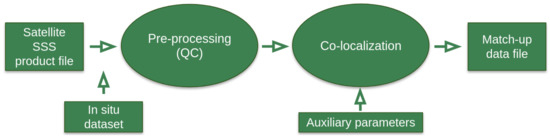
Figure 2.
Flow chart of the match-up generation.
3.1.1. In Situ/Satellite Data Preprocessing
The first step consists of filtering in situ data using the quality flags as described in Section 2.1 so that only valid salinity data remain in the final match-up files.
For high-spatial resolution in situ SSS measurements such as the thermosalinograph (TSG) SSS data, as well as SSS data from surface drifters, an additional spatial filtering step is performed on the in situ data that will be eventually compared to the satellite SSS products. If is the spatial resolution of the satellite SSS product (L2 to L3–L4), the in situ data are spatially low-pass filtered using a running median filter with a window width = to try to minimize the spatial representation uncertainty when compared to the lower spatial resolution of the satellite SSS product. Both original and filtered in situ data are finally stored in the MDB files.
For L2 satellite SSS data only, a third sub-step consists of filtering spurious data using the flags and associated recommendations as provided by the official data centers.
3.1.2. In Situ/Satellite Co-Localization
In this step, each SSS satellite acquisition is co-localized with the filtered in situ measurements. The method used for co-localization is different if the satellite SSS is a swath product (so-called Level 2-types) or a time-space composite product (so-called Level 3/Level 4 types).
- For L2 SSS swath data:If is the spatial resolution of the satellite swath SSS product, for each in situ data sample collected in the Pi-MEP database, the platform searches for all satellite SSS data found at grid nodes located within a radius of /2 from the in situ data location and acquired with a time-lag from the in situ measurement date that is less than or equal to ± 12 h. If several satellite SSS samples are found to meet these criteria, the final satellite SSS match-up point is selected to be the closest in time from the in situ data measurement date. The final spatial and temporal lags between the in situ and satellite data are stored in the MDB files.
- For L3 and L4 composite SSS products:If is the spatial resolution of the composite satellite SSS product and D the period over which the composite product was built (e.g., periods of 1, 7, 8, 9, 10, 18 days, 1 month, etc.) with central time , for each in situ data sample collected in the Pi-MEP database during the time interval [, ], the platform searches for all satellite SSS data of the composite product found at grid nodes located within a radius of /2 from the in situ data location. If several satellite SSS product samples are found to meet these criteria, the final satellite SSS match-up point is chosen to be the composite SSS with central time which is the closest in time from the in situ data measurement date. The final spatial and temporal lags between the in situ and satellite data are stored in the MDB files.
Recently, in the context of the evolving partnership with NASA, the Pi-MEP also provides an additional co-localization criterion that is applied only to L2 products, namely the “L2-Averaged” product match-ups. It consists of averaging all SSS L2 swath pixels falling in a spatio-temporal window defined by = 50 km and days around the in situ location. The spatial and temporal lags stored in the MDB files correspond to the average of all lags for each in situ datum.
3.1.3. MDB Pair Co-Localization with Auxiliary Data and Complementary Information
MDB data consist of satellite and in situ SSS pairs but also of auxiliary geophysical parameters such as the local history of wind speed and rain rates, as well as various pieces of information (climatology, distance to coast, mixed layer depth, barrier layer thickness, etc.) that can be derived from in situ, model, or satellite data and which are included in the final match-up files. The collocation of auxiliary parameters and additional information is carried out for each in situ SSS measurement contained in the match-up files as follows:
If is the time/date at which the in situ measurement is performed, we collect:
- The ASCAT wind speed product of the same day found at the ASCAT 1/4 grid node that is closest to the in situ data location. We then store the time series of the ASCAT wind speed at the same node for the 10 days prior to the in situ measurement day.
- If the in situ data are located within the 60N–60S band, we select the CMORPH 3-hourly product that is closest in time from and found at the CMORPH 1/4 grid node that is the closest distance from the in situ data location. We then store the time series of the CMORPH rain rate at the same node for 10 days prior to the in situ measurement time.
For the given month/year of the in situ data, we selected the ISAS and WOA fields for the same month (and same year for ISAS fields) and take the SSS analysis (monthly mean, STD) found at the closest grid node from the in situ measurement.
The distance from the in situ SSS data location to the nearest coast is evaluated and provided in km. We use a distance-to-coast map at 1/4 resolution where small islands have been removed.
When vertical profiles of salinity (S) and temperature (T) along depth (z) are made available from the in situ measurements used to build the match-up (Argo or marine mammals), the following variables are also included in each satellite/in situ match-up file:
- The vertical distribution of pressure at which the profiles were measured;
- The vertical S(z) and T(z) profiles;
- The vertical potential density anomaly profile ;
- The mixed layer depth (MLD). The MLD is defined here as the depth where the potential density has increased from the reference depth (10 meter) by a threshold equivalent to 0.2 C decrease in temperature at constant salinity: with , where and are the temperature and salinity at the reference depth (i.e., 10 m) [32,33];
- The top of the thermocline depth (TTD) is defined as the depth at which temperature decreases from its 10 m-depth value by 0.2 C;
- The barrier layer thickness (BLT) is defined as the difference between the MLD and the TTD. If BLT < 0, it corresponds to a vertically density compensated layer whose thickness is then the absolute value of (TTD-MLD);
- The vertical profile of the buoyancy frequency .
The resulting match-ups files are serialized as NetCDF-4 files whose structures depend on the origin of the in situ data.
3.2. Match-Up Characteristics for Each Specific In Situ/Satellite Pair
Several features/metrics of the MDB classified for each in situ/satellite/region triplet available are exhaustively described in each report generated. To illustrate what’s available in the reports, a sketchy listing of some of the latter are described below for a specific in situ dataset (Argo), satellite product (CCI SSS L4 Merged-OI v3.2—30-day running (ESA)) and Pi-MEP region (Global). The following section focuses on a general description of some of the available metrics, rather than on the geophysical interpretation of the obtained results.
3.2.1. Number of Paired SSS Data as a Function of Time and Distance to Coast
Figure 3 shows the time (left) and distance to coast (right) distributions of the match-ups between Argo and CCI SSS L4 Merged-OI v3.2—30-day running (ESA) for the Global Pi-MEP region and for the full satellite product period.

Figure 3.
Number of match-ups between Argo and CCI SSS L4 Merged-OI v3.2—30-day running (ESA) SSS as a function of time (left) and as a function of the distance to coast (right) over the Global Pi-MEP region and for the full satellite product period.
3.2.2. Histograms of the SSS Match-Ups
Figure 4 shows the SSS distribution of Argo (left) and CCI SSS L4 Merged-OI v3.2—30-day running (ESA) (right) considering all match-up pairs per bins of 0.1 pss over the Global Pi-MEP region and for the full satellite product period.
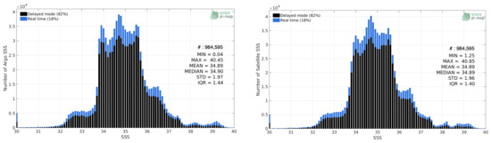
Figure 4.
Histograms of SSS from Argo (left) and CCI SSS L4 Merged-OI v3.2—30-day running (ESA) (right) considering all match-up pairs per bins of 0.1 over the Global Pi-MEP region and for the full satellite product period.
3.2.3. Distribution of In Situ SSS Depth Measurements
Figure 5 shows the depth distribution of the upper level SSS measurements from Argo in the Match-up Data Base for the Global Pi-MEP region (left) and temporal mean spatial distribution of pressure of the in situ SSS data over 11 boxes and for the full satellite product period (right).

Figure 5.
Histograms of the depth of the upper level SSS measurements from Argo in the Match-up Data Base for the Global Pi-MEP region (left) and temporal mean spatial distribution of pressure of the in situ SSS data over 11 boxes and for the full satellite product period (right).
3.2.4. Spatial Distribution of Match-Ups
In Figure 6, we show the distribution of SSS match-ups between Argo SSS and the CCI SSS L4 Merged-OI v3.2—30-day running (ESA) SSS product for the Global Pi-MEP region over 1 1 boxes and for the full satellite product period.

Figure 6.
Number of SSS match-ups between Argo SSS and the CCI SSS L4 Merged-OI v3.2—30-day running (ESA) SSS product for the Global Pi-MEP region over 1× 1 boxes and for the full satellite product period.
3.2.5. Histograms of the Spatial and Temporal Lags of the Match-Ups Pairs
Figure 7 reveals the spatial (left) and temporal (right) lags between the location/time of the Argo measurement and the position/date of the corresponding CCI SSS L4 Merged-OI v3.2—30-day running (ESA) SSS pixel of all match-ups pairs.

Figure 7.
Histograms of the spatial (left) and temporal (right) lags between the location/time of the Argo measurement and the position/date of the corresponding CCI SSS L4 Merged-OI v3.2—30-day running (ESA) SSS pixel.
3.3. Match-Up Analysis Report
In each report, the platform then provides an ensemble of results of analyses on the selected paired satellite/in situ SSS MDB. The figures presented are examples of the results obtained from the automated analysis of the MDB. The database will also enable additional analyses by users.
3.3.1. Spatial Maps of the Temporal Mean and STD of In Situ and Satellite SSS and of Their Difference (SSS)
In Figure 8, we show maps of temporal mean (left) and temporal standard deviation (right) of the CCI SSS L4 Merged-OI v3.2—30-day running (ESA) (top) and of the Argo in situ dataset at the collected Pi-MEP match-up pairs. The temporal mean and STD are gridded over the full satellite product period and over spatial boxes of size 11.

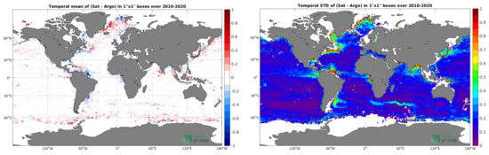
Figure 8.
Temporal mean (left) and STD (right) of SSS from CCI SSS L4 Merged-OI v3.2—30-day running (ESA) (top), Argo (middle), and of SSS (Satellite—Argo) (bottom). Only match-up pairs are used to generate these maps.
At the bottom of Figure 8, the temporal mean (left) and standard deviation (right) of the differences between the satellite SSS product and in situ data found at match-up pairs, namely SSS (Satellite—Argo), is also gridded over the full satellite product period and over spatial boxes of size 11.
3.3.2. Time Series of the Monthly Median and STD of In Situ and Satellite SSS and of Their Difference (SSS)
In the top panel of Figure 9, we show the time series of the monthly median SSS estimated over the full Global Pi-MEP region for both CCI SSS L4 Merged-OI v3.2—30-day running (ESA) satellite SSS product (in black) and the Argo in situ dataset (in blue) at the collected Pi-MEP match-up pairs.
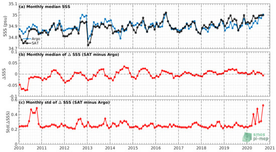
Figure 9.
Time series of the monthly median SSS, median of SSS (Satellite—Argo) and STD of SSS (Satellite—Argo) over the Global Pi-MEP region considering all match-ups collected by the Pi-MEP.
In the middle panel of Figure 9, we show the time series of the monthly median of the SSS difference SSS (Satellite—Argo) for the collected Pi-MEP match-up pairs and estimated over the full Global Pi-MEP region.
In the bottom panel of Figure 9, we show the time series of the monthly standard deviation of the SSS difference SSS (Satellite—Argo) for the collected Pi-MEP match-up pairs and estimated over the full Global Pi-MEP region.
3.3.3. Zonal Mean and STD of In Situ and Satellite SSS and of Their Difference (SSS)
In Figure 10 on the left panel, we show the zonal mean SSS considering all Pi-MEP match-up pairs for both CCI SSS L4 Merged-OI v3.2—30-day running (ESA) satellite SSS product (in black) and the Argo in situ dataset (in blue). The full satellite SSS product period is used to derive the mean.

Figure 10.
Left panel: Zonal mean SSS from CCI SSS L4 Merged-OI v3.2—30-day running (ESA) satellite product (black) and from Argo (blue). Right panel: Zonal mean of SSS (Satellite—Argo) for all the collected Pi-MEP match-up pairs estimated over the full satellite product period.
In the right panel of Figure 10, we show the zonal mean of SSS (Satellite—Argo) for all the collected Pi-MEP match-up pairs estimated over the full satellite product period.
3.3.4. Scatterplots of Satellite versus In Situ SSS by Latitudinal Bands
In Figure 11, contour maps of the concentration of CCI SSS L4 Merged-OI v3.2—30-day running (ESA) SSS (y-axis) versus Argo SSS (x-axis) at match-up pairs for different latitude bands are shown: (a) 80S–80N, (b) 20S–20N, (c) 40S–20S and 20N–40N and (d) 60S–40S and 40N–60N. For each plot, the red line shows x = y. The black thin and dashed lines indicate a linear fit through the data cloud and the ±95% confidence levels, respectively. In the figure, the value of n represents the number of match-up pairs between the CCI and in situ SSS. The values for the slope and R2 coefficient are the results of the linear fit between the CCI and in situ SSS match-up data. The root mean squared (RMS) values indicate the RMS difference between the CCI and in situ data. The bias denotes the mean difference between the CCI and in situ data.
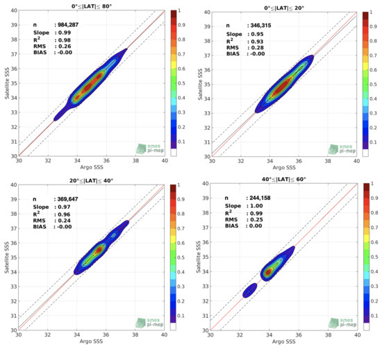
Figure 11.
Contour maps of the concentration of CCI SSS L4 Merged-OI v3.2—30-day running (ESA) SSS (y-axis) versus Argo SSS (x-axis) at match-up pairs for different latitude bands. For each plot, the red line shows x = y. The black thin and dashed lines indicate a linear fit through the data cloud and the ±95% confidence levels, respectively.
3.3.5. Time Series of the Monthly Median and STD of SSS Sorted by Latitudinal Bands
In Figure 12, the time series of the monthly median (red curves) of SSS (Satellite—Argo) and ±1 STD (black vertical thick bars) as a function of time for all the collected Pi-MEP match-up pairs estimated over the Global Pi-MEP region and for the full satellite product period are shown for different latitude bands is shown: (a) 80S– 80N, (b) 20S–20N, (c) 40S–20S and 20N–40N and (d) 60S–40S and 40N–60N.
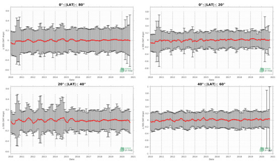
Figure 12.
Monthly median (red curves) of SSS (Satellite—Argo) and ±1 STD (black vertical thick bars) as function of time for all the collected Pi-MEP match-up pairs estimated over the Global Pi-MEP region and for the full satellite product period are shown for different latitude bands: (a) 80S–80N, (b) 20S–20N, (c) 40S–20S and 20N–40N and (d) 60S–40S and 40N–60N.
3.3.6. SSS Sorted as a Function of Geophysical Parameters
In Figure 13, we classify the match-up differences SSS (Satellite—in situ) between CCI SSS L4 Merged-OI v3.2—30-day running (ESA) and Argo SSS as a function of the geophysical conditions at match-up points. The median and STD of SSS (Satellite—Argo) is thus evaluated as a function of the
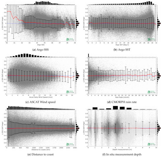
Figure 13.
SSS (Satellite—Argo) sorted as function of Argo SSS values (a), Argo SST (b), ASCAT Wind speed (c), CMORPH rain rate (d), distance to coast (e) and in situ measurement depth (f). In all plots the median and STD of SSS for each bin is indicated by the red curves and black vertical thick bars (±1 STD). Normalized marginal histograms are also indicated outside each plot.
- In situ SSS values per bins of width 0.2;
- In situ SST values per bins of width 1 C;
- ASCAT daily wind values per bins of width 1 m/s;
- CMORPH 3-hourly rain rates per bins of width 1 mm/h;
- Distance to coasts per bins of width 50 km;
- In situ measurement depth (if relevant).
4. Exploitation: Tools and Case Studies
Several tools to inspect, analyze and compare the platform results have been developed or adapted for the Pi-MEP project. The main tools are: Syntool (web application to visualize data collections), plot interface (plotting satellite data products characteristics) and MDB interface (plotting match-ups statistics), and Merginator (web application to explore maps of multiple variables). Additionally, several case studies have been identified for the scientific exploitation of specific oceanographic processes and regions. Further, a Jupyter notebook has been specifically developed to access and process Pi-MEP data. To learn how to use this application, you can check out this quick start guide (https://pimep.ifremer.fr/diffusion/docs/pimep_quick_start_guide_plot-mdb-merginator_interfaces.pdf, accessed on 9 November 2021).
4.1. Syntool
Syntool is a web application to explore and visualize collections of satellite, in situ and model data (Figure 14). By rendering various sources of data on the same map, it aims to reveal synergies and coherencies/incoherencies between multiple datasets. The main component of the Syntool application is a cartographic view which takes most of the available screen space. This view is built upon the widely used OpenLayers library which has been tested on most platforms and web browsers. This library can load data using most GIS protocols (TMS, WMS, etc.), render them on a 2D map and let users move the map around by dragging it with the mouse or zoom to a specific area by using the mouse wheel. Pi-MEP core datasets (satellite, model and in situ) are made available on Syntool as well as the listed ocean surface currents, sea surface temperature, wind speed and precipitation products.
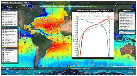
Figure 14.
Illustration of Syntool data portal interface: The selection of products to be displayed is controlled by the left “Products” menu. The date and time selection is controlled by the lower banner (timeline). The mouse scroll controls zoom levels while on the map and time while on the timeline. Dates when selected products are available appear in white, or grey otherwise. When activating the collocation trigger, dates when all selected products are available within the time range and the visible map area appear in red.
4.2. Plot Interface
The plot interface (Figure 15) allows for a quick visualization of most SSS products included in the Pi-MEP. Based on Big Data technology for the efficient storage and manipulation of georeferenced data, this interface computes statistics and generate plots on the fly.
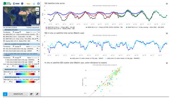
Figure 15.
Illustration of the plot interface: The left side contains the controls (selection of an area on the map and a time period, the satellite/in situ products to be analyzed) and the right side contains the resulting plots.
It contains the controls for selecting an area and a time range, for adding a new plot and for the configuration of each type of plot: (multi-)time series, scatter plots, and map charts. All plots can be exported as PNG images to be easily embedded in documents. Time series, scatter plots and histograms provide some additional interactivity to focus on a sub-domain (zoom/pan) or a specific data point (value under cursor). A menu also offers the possibility to download the data as CSV files for these latter plots.
4.3. Match-Up Interface
Searching match-ups and extracting the associated data is made easy using this tool (Figure 16). The match-up database (MDB) interface contains a form to define the search filters (spatial box, temporal window, satellite product, in situ dataset, distance to coast, etc.) and provides means to visualize the results through specific plots, also allowing one to download them as CSV files.
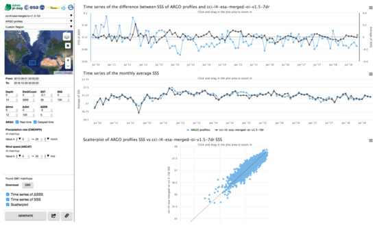
Figure 16.
Illustration of the MDB interface.
Before performing a search or an extraction, the interface requires the user to select an in situ/satellite couple, an area (from the list of preset Pi-MEP regions) and a time range. A user-defined spatial domain can also be selected using the rectangle and zoom functions on the map. More advanced filters are also available but are locked until the in situ/satellite couple has been selected since some options are specific to a satellite or an in situ sensor. These include the potential selection of the:
- Depth of in situ measurements (between 0 and 10 m);
- Distance to coast (from 0 to 5000 km);
- SST range of the extraction in situ (from −2.1 to 35 C);
- SSS range of the extraction in situ (from 0 to 45);
- Temporal lag in the collocation process between the in situ date and SSS satellite data (between −16 and 16 days);
- Spatial lag in the collocation process between the in situ date and SSS satellite data (between 0 and 100 km);
- Real-time or delay mode or both (for Argo only);
- CMORPH rain rate at the time and location of the in situ measurement: filter if it is superior or inferior to a specified threshold (from 0 to 100 mm/h);
- ASCAT wind speed at the time and location of the in situ measurement: filter if it is superior/inferior to a specified threshold (from 0 to 30 m/s);
- Difference between in situ and satellite SSS values range (−5 to 5).
4.4. Merginator
In many situations, scientists want to compare data collocated on specific regions and time periods (visually at least). Merginator is a web application (Figure 17) using the full catalog of Pi-MEP datasets to build thematic web interfaces mixing different sources of products (satellites L2 to L4, in situ, model), performing collocation and generating images on the fly.

Figure 17.
Illustration of the Merginator interface.
4.5. Jupyter Notebooks
A Jupyter notebook is a web interface where users can write documents that contain code, text, equations, plots and rich media. By default, code is executed remotely on the web server but the notebook server can be configured to delegate code execution to machines which have both access to the data and to the web server, which is a better option for scalable infrastructures. By default, only Python code is supported, but Jupyter has a modular design and other languages can be added by installing plugins. The notebooks server offered by the Pi-MEP gives users the possibility to develop and execute their own algorithms within a Python environment with preinstalled modules for scientific processing and with access to a large amount of data. Due to the remote execution mechanism, code written by users has direct access to the Pi-MEP files and can produce results without requiring the transfer of a potentially high volume of input data. For logistic and security reasons, only authenticated users are allowed to execute notebooks on the platform.
4.6. Case Studies
The Pi-MEP also intends to enhance the value of the SMOS, Aquarius and SMAP missions by monitoring and characterizing a series of selected illustrative process studies in crucial oceanographic areas. Upon consultation with the SAG at the beginning of the project, the following case studies have been identified and are currently portrayed in the platform:
- SSS monitoring of large river plumes [34];
- Mesoscale SSS signatures in the Western boundary current [35];
- SSS at high latitudes and semi-enclosed seas [36];
- SSS in rainy oceanic regions: the SPURS-2 field campaign [37].
To this end, the Pi-MEP website contains dedicated web pages for each of the selected case studies, where users can find analyses and results, up-to-date plots and reports, as well as regionally dedicated visualization/extraction tools. In addition, in these pages users have access to (1) an up-to-date literature review on SSS remote sensing for the given case study, with links to published reference papers, (2) the SSS in situ/satellite match-up files and reports generated over the chosen case study region, and (3) specific and dedicated scientific analyses for each case study, as detailed hereafter.
4.6.1. Case Study 1: Monitoring of Large River Plumes
Large rivers are key hydrologic components in oceanography, particularly regarding air–sea and land–sea exchanges and biogeochemistry. Despite this importance, tracing major river water over large distances in the ocean was not straightforward before the satellite SSS era, principally due to a lack of in situ SSS observations in these highly dynamical zones. Being able to routinely monitor the dispersal patterns of river plumes, their spatial extension and mixing rates as well as co-variabilities with ocean color, surface winds and currents is now feasible thanks to SMOS, Aquarius/SAC-D and SMAP SSS data. Four regional case studies of “river plumes” focusing on the world’s largest rivers in terms of discharge are proposed on the platform, i.e., the Amazon and Orinoco, Congo and Niger, Mississippi, Ganges and Brahmaputra rivers (Figure 18).
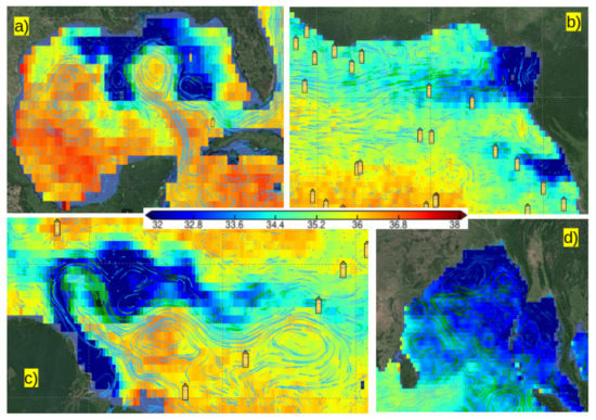
Figure 18.
Illustration of the river plumes using Syntool: (a) Mississippi, (b) Congo/Niger, (c) Amazon/Orinoco, and (d) Ganges and Brahmaputra rivers. Colors correspond to SSS data coming from different satellite products available in the portal. The streamlines represent the geostrophic currents and the yellow bottles icons in (a–c) indicate Argo floats locations.
Users can generate their own SSS time series (satellite/in situ) and plots on a given spatial domain around each river mouth, or at a virtual buoy (point) in these regions. Time series are compared to the amplitude of the annual cycle of the river discharges. The visualization of the seasonal and interannual co-variabilities (correlation) between spatial patterns of satellite SSS, absorption coefficient of CDOM at 443 nm, precipitation, and surface winds are provided either after averaging all years or year by year. The coherency between the different satellite SSS products and surface currents from combined altimetry, wind, and SST data (Globcurrent products) in the river plume regions can also be monitored using the Syntool visualization software. To further investigate the capability of the satellite SSS estimates to help monitor the horizontal distribution of the vertical density stratification over the river plume waters, the platform finally evaluates how correlated the satellite SSS and/or SST values in the plume waters are with the strength of the vertical stratification below the plume and surrounding waters, as determined from Argo floats.
4.6.2. Case Study 2: Mesoscale Signatures in Western Boundary Currents
The advent of satellite measurements of SSS provides a unique opportunity to study the spatio-temporal behavior of SSS in association with mesoscale oceanic features in Western boundary currents from synoptic to interannual time scales. The coherency between the different satellite SSS products and surface currents in the Gulf Stream (GS) region can be monitored from the platform using the Syntool visualization software. The monitoring of the SSS and SST fronts in the Gulf stream region from satellite data (Figure 19) are also systematically compared to the fronts provided by the numerical model forecasts from the Mercator (CMEMS) model. The platform provides time--latitude Hovmöller diagrams of Satellite SSS, AVISO SLA, AVHRR SST, and Chlorophyll-A (from Globcolour) along two zonal transects at longitude 65W and 50W, which are at two key positions of the Gulf-stream westward flow. The user can visualize the results for the different years.
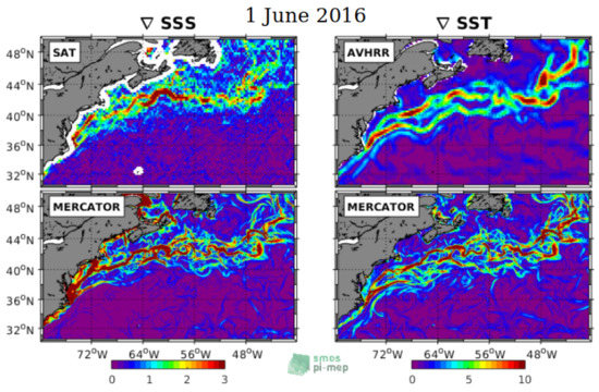
Figure 19.
Gradients of monthly averaged SSS (left) and SST (right) maps from CCI SSS product and AVHRR (top), and from Mercator (bottom) operational forecast system.
A covariance analysis of the high-pass filtered SSS, SSH, and SST fields within two 5× 5 boxes along the GS path is accessible from the platform. The filter is defined by removing from the fields the mean large-scale (>300 km) background flow. The results allow one to monitor the variability of the correlations between SSS and sea level variability in comparison to the ones between SST and SSH.
4.6.3. Case Study 3: High-Latitude and Semi-Enclosed Seas
Retrieving SSS from L-band radiometers in the Antarctic regions is especially challenging due to (1) a significantly lower sensitivity of changes in brightness temperature to changes in SSS at relatively low SST; (2) the influence of the strong winds of the high-latitude Southern Hemisphere on the brightness temperature; and (3) the potential contamination of the radiometer data by sea ice. Despite the potential inaccuracies of satellites and differences within the satellite salinity products, the increased temporal and spatial scales and measuring the top few centimeters of the ocean surface have made satellite-derived salinity a useful quantity for air–sea interaction studies. The platform provides literature review, satellite/in situ match-up pairs in the region and visualization tools to monitor the concurrent SST and surface currents.
The Mediterranean Sea is one of the most challenging world regions to retrieve salinity from L-band satellite observations mainly due to two reasons: the land–sea contamination and the degradation of the measurements due to the effect of the radio frequency interference (RFI) sources, which are particularly frequent in the Eastern Mediterranean. First analyses have attempted to provide better filtered and quality-controlled SMOS products in these regions and help quantifying eddies activity in the western Mediterranean Sea. SMAP data, being better protected from RFI, show promising quality in this region and were used to study the SSS tendency in the basin. In addition, the time-evolution of satellite SSS and evaporation (OAflux) minus precipitation (CMORPH) is provided in the Mediterranean Sea (Figure 20).
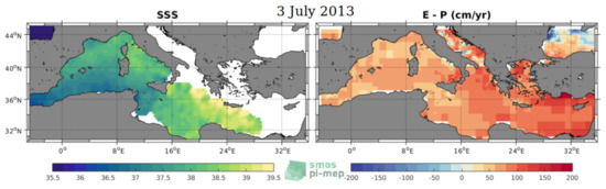
Figure 20.
Satellite SSS (SMOS L3 MED-ATL-OA V2—9 DAYS (BEC)) and Evaporation (OAflux) minus precipitation (CMORPH) estimates in the Mediterranean Sea.
4.6.4. Case Study 4: Salinity Processes in the Upper-Ocean Regional Studies (SPURS-2) Field Experiment
The 2016–2017 Salinity Processes in the Upper-ocean Regional Studies (SPURS-2) field experiment sampled the westward extension of the Eastern tropical Pacific Fresh Pool (EPFP). This is a low-surface salinity feature which extends westward from the coast of Panama and Colombia. It contains some of the freshest surface water in the global ocean due to runoff from rivers in Central America and atmospheric transport of freshwater from the Atlantic across the Central American isthmus (Figure 21). The EPFP is also associated with the intertropical convergence zone (ITCZ). This is a band of converging air, thick clouds and heavy rain, which makes seasonal excursions between the equator and about 10N.

Figure 21.
From [38], Sea surface salinity for the month of September 2017 from SMAP satellite data. The SPURS-2 site is indicated by an arrow.
The purpose of SPURS-2 was to elucidate the relationship between rainfall, ocean dynamics and surface salinity. Rainfall in the region is heavy on average, but also very patchy and seasonal. When it does rain, the freshwater input into the ocean is buoyant and tends to lie at the surface in very thin (<5 m) fresh puddles for some period of time before it mixes into the ocean below. How these small-scale puddles combine with the larger-scale current systems to generate the low-salinity feature at the surface that stretches across the entire tropical Pacific is still a debated subject. Additional relevant questions consider how large the near-surface salinity stratification induced by rainfall is and how this stratification depends on rain rate and wind speed (that causes vertical mixing). Moreover, the patchiness of rainfall and the small-scale ocean dynamics also results in small-scale variation of SSS within satellite footprints, namely, sub-footprint variability (SFV). SFV can lead to differences between the “match-up” of satellite SSS (averaged over satellite footprints) and pointwise in situ measurements due to the differences in spatial scales resolved by satellites and in situ platforms as well as their temporal sampling mismatch.
This case study is still under development and analyses on the impact of vertical SSS stratification on the differences between satellite and in situ data, as well as some links between SSS, rain and winds, shall be provided in the near future.
5. Summary and Conclusions
Although SMOS, the first of the series of satellite missions dedicated to sea surface salinity observations, was launched more than 12 years ago (November 2009–now), estimating SSS from L-band orbiting radiometers remains a relatively young and challenging field of oceanography from space. In comparison, developments achieved in sea level, sea surface temperature, or ocean color monitoring are indeed now more than 50 years old. Nevertheless, our knowledge of the very near-surface salinity global variability dramatically improved thanks to these missions ([1,2]). A rich panel of research and development activities were conducted in the last decade by international teams involved in the three above-mentioned missions. These include brightness temperature data calibration, retrieval algorithms and radiative transfer forward models adjustments/developments, bias corrections, product validation, and specific analyses in scientific case studies. These key activities all involve the combined use of satellite and ground truth in situ observations of sea surface salinity. Validating the large-footprint-size quasi-instantaneous satellite SSS observations, or their space-time composites (e.g., monthly average) with very local (in space and time) upper ocean in situ observations of the salinity, however, remains a challenge [39].
On the one hand, a large ensemble of in situ SSS data distributed by different data centers are available to infer SMOS, Aquarius, and SMAP SSS products’ quality. The sources of in situ SSS data include Argo floats, moored buoys, thermosalinographs installed on voluntary observing ships, research vessels and sailing ships, surface drifters, and equipped marine mammals, as well as dedicated campaigns data and analyzed in situ data fields.
On the other hand, numerous satellite SSS datasets and validation approaches have been produced by the different SMOS, Aquarius and SMAP ground segments, and also by the associated missions’ expertise groups or users from the scientific community. This heterogeneity is explained by the exploratory nature of the satellite SSS missions, their new instrumental concepts and the outcomes of the first spaceborne SSS measurements. As an example of this diversity, there are about 10 satellite SSS data production centers for the three missions and an ensemble of 28 global and 8 regional satellite SSS products. The variety of approaches developed is in response to the multiplicity of scientific challenges faced at different processing levels by different data center teams. The absolute accuracy of the satellite SSS measurements is significantly less than automated in situ sensors. Moreover, they are not sensing the same layers of the upper ocean. Therefore, the satellite and in situ observing systems complement each other when their respective merits are capitalized.
Measurement complexity and heterogeneous data quality and sampling are two identified major issues limiting the confidence users might have in the relatively young satellite SSS products. In this context, the Pilot-Mission Exploitation Platform (Pi-MEP) for ocean surface salinity has been developed and operated since 2018 to provide scientists and other potential users with an ensemble of tools and functionalities that grant the level of expertise satellite people (from SMOS, Aquarius, or SMAP missions science teams) might already have. One aim of the platform is also to ease access to the necessary data ensemble that will foster and develop the user’s ability to perform rapidly interesting and new scientific exploitations of the satellite SSS data. The Pi-MEP is designed to allow systematic comparisons between available datasets by providing comparable quality control metrics applied for all the satellite-derived SSS products. In particular, Pi-MEP enables users to:
- Choose which satellite SSS product is best adapted for their own specific application;
- Improve the Level 2 to Level 4 SSS retrieval algorithms by better systematically identifying the conditions for which a given satellite SSS product is of good or degraded quality;
- Eventually converge towards the best validation and retrieval algorithm approaches and generate fewer satellite SSS products but with increased quality.
The platform was therefore designed to provide the user with a complete and configurable geophysical characterization within a requested space-time domain of observations. This shall drive the user’s interest to further analyze the data, favoring the learning capability of new users and increasing the user confidence in the SSS data themselves by enabling physical consistency checks between ensembles of multiple EO observations.
Under the recommendations and requirements raised by a community-driven science advisory group, an ensemble of satellite and in situ data have been collected on the platform around about 37 well-referenced satellite SSS products. Data quality controls have been applied to both satellite and in situ data and systematic validation methodologies have been implemented to produce and give access to the so-called “Match-up DataBase (MDB)” files, including co-localized values between each satellite and in situ datasets as well as environmental and acquisition parameters. These MDB data are collected since the beginning of operation of each satellite mission and used to produce systematic validation reports including an ensemble of data quality monitoring analyses. In addition, an ensemble of data visualization and extraction tools are provided by the platform enabling user-driven specific analyses.
All satellite and in situ data SSS already available in the Pi-MEP were detailed in the present paper. The platform content is dynamic and updated twice per year to include new products (e.g., satellite product reprocessings and new releases, new campaign data) and to complete existing time series and associated reports and analyses [40]. We plan to add new features to the platform on several technical aspects, such as triple-collocation software implementation, spatial spectral analyses and sustained exploitation of data from the SPURS campaigns.
Author Contributions
Conceptualization, S.G., N.R. and R.S.; methodology, S.G. and N.R.; software, S.G., S.H., Z.E.K.H., J.-F.P. and F.P.; formal analysis, S.G. and N.R.; investigation, S.G. and N.R.; data curation, S.G.; writing original draft preparation, S.G.; writing, review and editing, N.R., R.S., T.L., J.J.S., F.M.B., D.L.V. and N.V.-S.; supervision, N.R.; project administration, R.S.; funding acquisition, S.M., K.S. and H.L. All authors have read and agreed to the published version of the manuscript.
Funding
This project is funded by ESA through the Earth Observation Envelope Programme.
Institutional Review Board Statement
Not applicable.
Informed Consent Statement
Not applicable.
Data Availability Statement
All data produced by Pi-MEP are freely available online and easily downloadable (https or ftp) via the web platform: https://www.salinity-pimep.org (accessed on 9 November 2021). All data used by the platform are described in the following web page: https://www.salinity-pimep.org/data/input.html (accessed on 9 November 2021) with the proper links to the data providers.
Acknowledgments
The authors would like to acknowledge SAG members for their support to the project and the three anonymous reviewers for their comments and suggestions.
Conflicts of Interest
The authors declare no conflict of interest.
Abbreviations
The following abbreviations are used in this manuscript:
| Aquarius | NASA/CONAE Salinity mission |
| ASCAT | Advanced Scatterometer |
| BLT | Barrier Layer Thickness |
| CCI | Climate Change Initiative |
| CMORPH | CPC MORPHing technique (precipitation analyses) |
| CPC | Climate Prediction Center |
| CTD | Instrument used to measure the conductivity, temperature, and pressure of seawater |
| DM | Delayed Mode |
| EO | Earth Observation |
| ESA | European Space Agency |
| FTP | File Transfer Protocol |
| GOSUD | Global Ocean Surface Underway Data |
| GTMBA | The Global Tropical Moored Buoy Array |
| Ifremer | Institut français de recherche pour l’exploitation de la mer |
| IPEV | Institut polaire français Paul-Émile Victor |
| ISAS | In Situ Analysis System |
| L2 | Level 2 |
| LEGOS | Laboratoire d’Etudes en Géophysique et Océanographie Spatiales |
| LOCEAN | Laboratoire d’Océanographie et du Climat: Expérimentations et |
| Approches Numériques | |
| LOPS | Laboratoire d’Océanographie Physique et Spatiale |
| MDB | Match-up Data Base |
| MEOP | Marine Mammals Exploring the Oceans Pole to Pole |
| MLD | Mixed Layer Depth |
| NCEI | National Centers for Environmental Information |
| NRT | Near Real Time |
| NTAS | Northwest Tropical Atlantic Station |
| OI | Optimal interpolation |
| Pi-MEP | Pilot-Mission Exploitation Platform |
| PIRATA | Prediction and Researched Moored Array in the Atlantic |
| QC | Quality control |
| Spatial resolution of the satellite SSS product | |
| RAMA | Research Moored Array for African-Asian-Australian Monsoon Analysis and |
| Prediction | |
| R | Square of the Pearson correlation coefficient: |
| RMS | Root mean square: |
| RR | Rain rate |
| SAMOS | Shipboard Automated Meteorological and Oceanographic System |
| Slope | Slope of a fitted line assuming an ordinary least squares regression model. |
| SMAP | Soil Moisture Active Passive (NASA mission) |
| SMOS | Soil Moisture and Ocean Salinity (ESA mission) |
| SPURS | Salinity Processes in the Upper Ocean Regional Study |
| SSS | Sea Surface Salinity |
| SSS | In situ SSS data considered for the match-up |
| SSS | Satellite SSS product considered for the match-up |
| SSS | Difference between satellite and in situ SSS at colocalized point |
| (SSS = SSS- SSS) | |
| SST | Sea Surface Temperature |
| STD | Standard deviation: |
| STD | Robust Standard deviation = median(abs(x-median (x)))/0.67 (less affected |
| by outliers than STD) | |
| Stratus | Surface buoy located in the eastern tropical Pacific |
| Survostral | SURVeillance de l’Océan AuSTRAL (Monitoring the Southern Ocean) |
| TAO | Tropical Atmosphere Ocean |
| TSG | ThermoSalinoGraph |
| WHOI | Woods Hole Oceanographic Institution |
| WHOTS | WHOI Hawaii Ocean Time-series Station |
| WOA | World Ocean Atlas |
References
- Reul, N.; Grodsky, S.A.; Arias, M.; Boutin, J.; Catany, R.; Chapron, B.; D’Amico, F.; Dinnat, E.; Donlon, C.; Fore, A.; et al. Salinity estimates from Spaceborne L-band radiometers: An overview of the first decade of observation (2010–2019). Remote Sens. Environ. 2020, 242, 111769. [Google Scholar] [CrossRef]
- Vinogradova, N.; Lee, T.; Boutin, J.; Drushka, K.; Fournier, S.; Sabia, R.; Stammer, D.; Bayler, E.; Reul, N.; Gordon, A.; et al. Satellite Salinity Observing System: Recent Discoveries and the Way Forward. Front. Mar. Sci. 2019, 6, 243. [Google Scholar] [CrossRef]
- Kilic, L.; Prigent, C.; Aires, F.; Boutin, J.; Heygster, G.; Tonboe, R.T.; Roquet, H.; Jimenez, C.; Donlon, C. Expected Performances of the Copernicus Imaging Microwave Radiometer (CIMR) for an All-Weather and High Spatial Resolution Estimation of Ocean and Sea Ice Parameters. J. Geophys. Res. 2018, 123, 7564–7580. [Google Scholar] [CrossRef] [Green Version]
- Pi-MEP. Match-up Datasets. 2021. Available online: https://www.salinity-pimep.org/data/mdb.html (accessed on 15 September 2021).
- Pi-MEP. Match-up Reports. 2021. Available online: https://www.salinity-pimep.org/reports/mdb.html (accessed on 15 September 2021).
- Pi-MEP. In-Situ Reports. 2021. Available online: https://www.salinity-pimep.org/reports/insitu.html (accessed on 15 September 2021).
- Gaillard, F.; Reynaud, T.; Thierry, V.; Kolodziejczyk, N.; von Schuckmann, K. In Situ-Based Reanalysis of the Global Ocean Temperature and Salinity with ISAS: Variability of the Heat Content and Steric Height. J. Clim. 2016, 29, 1305–1323. [Google Scholar] [CrossRef]
- Argo. Argo Float Data and Metadata from Global Data Assembly Centre (Argo GDAC). SEANOE 2021. [Google Scholar] [CrossRef]
- Alory, G.; Delcroix, T.; Téchiné, P.; Diverrès, D.; Varillon, D.; Cravatte, S.; Gouriou, Y.; Grelet, J.; Jacquin, S.; Kestenare, E.; et al. The French contribution to the voluntary observing ships network of sea surface salinity. Deep-Sea Res. Pt. I 2015, 105, 1–18. [Google Scholar] [CrossRef]
- Kolodziejczyk, N.; Diverres, D.; Jacquin, S.; Gouriou, Y.; Grelet, J.; Le Menn, M.; Tassel, J.; Reverdin, G.; Maes, C.; Gaillard, F. Sea Surface Salinity from French RESearcH Vessels: Delayed Mode Dataset, Annual Release. SEANOE 2020. [Google Scholar] [CrossRef]
- Reynaud, T.; Desprez De Gesincourt, F.; Gaillard, F.; Le Goff, H.; Reverdin, G. Sea Surface Salinity from Sailing Ships: Delayed Mode Dataset, Annual Release. SEANOE 2017. [Google Scholar] [CrossRef]
- Smith, S.R.; Rolph, J.J.; Briggs, K.; Bourassa, M.A. Quality-Controlled Underway Oceanographic and Meteorological Data from the Center for Ocean-Atmospheric Predictions Center (COAPS)—Shipboard Automated Meteorological and Oceanographic System (SAMOS). NOAA Natl. Cent. Environ. Inf. Dataset. 2009. [Google Scholar] [CrossRef]
- Morrow, R.; Kestenare, E. Nineteen-year changes in surface salinity in the Southern Ocean south of Australia. J. Mar. Sys. 2014, 129, 472–483. [Google Scholar] [CrossRef]
- Aulicino, G.; Cotroneo, Y.; Ansorge, I.; Van Den Berg, M. Sea Surface Temperature and Salinity Collected Aboard the S.A. AGULHAS II and S.A. AGULHAS in the South Atlantic Ocean and Southern Ocean from 2010-12-08 to 2017-02-02 (NCEI Accession 0170743). NOAA Natl. Cent. Environ. Inf. Dataset 2018. [Google Scholar] [CrossRef]
- Morisset, S.; Reverdin, G.; Boutin, J.; Martin, N.; Yin, X.; Gaillard, F.; Blouch, P.; Rolland, J.; Font, J.; Salvador, J. Surface salinity drifters for SMOS validation. Mercator Ocean—CORIOLIS Q. Newsl. 2012, 45, 33–37. [Google Scholar]
- Treasure, A.; Roquet, F.; Ansorge, I.; Bester, M.; Boehme, L.; Bornemann, H.; Charrassin, J.B.; Chevallier, D.; Costa, D.; Fedak, M.; et al. Marine Mammals Exploring the Oceans Pole to Pole: A Review of the MEOP Consortium. Oceanography 2017, 30, 132–138. [Google Scholar] [CrossRef]
- Roquet, F.; Guinet, C.; Charrassin, J.B.; Costa, D.P.; Kovacs, K.M.; Lydersen, C.; Bornemann, H.; Bester, M.N.; Muelbert, M.C.; Hindell, M.A.; et al. MEOP-CTD In-Situ Data Collection: A Southern Ocean Marine-Mammals Calibrated Sea Water Temperatures and Salinities Observations. SEANOE 2018. [Google Scholar] [CrossRef]
- Roemmich, D.; Gilson, J. The 2004–2008 mean and annual cycle of temperature, salinity, and steric height in the global ocean from the Argo Program. Prog. Oceanogr. 2009, 82, 81–100. [Google Scholar] [CrossRef]
- Boutin, J.; Chao, Y.; Asher, W.E.; Delcroix, T.; Drucker, R.; Drushka, K.; Kolodziejczyk, N.; Lee, T.; Reul, N.; Reverdin, G.; et al. Satellite and In Situ Salinity: Understanding Near-Surface Stratification and Sub-footprint Variability. Bull. Am. Meterol. Soc. 2016, 97, 1391–1407. [Google Scholar] [CrossRef] [Green Version]
- Joyce, R.J.; Janowiak, J.E.; Arkin, P.A.; Xie, P. CMORPH: A Method that Produces Global Precipitation Estimates from Passive Microwave and Infrared Data at High Spatial and Temporal Resolution. J. Hydrometeorol. 2004, 5, 487–503. [Google Scholar] [CrossRef]
- Bentamy, A.; Grodsky, S.A.; Carton, J.A.; Croizé-Fillon, D.; Chapron, B. Matching ASCAT and QuikSCAT winds. J. Geophys. Res. 2012, 117. [Google Scholar] [CrossRef] [Green Version]
- Banzon, V.; Smith, T.M.; Steele, M.; Huang, B.; Zhang, H.M. Improved Estimation of Proxy Sea Surface Temperature in the Arctic. J. Atmos. Oceanic Technol. 2020, 37, 341–349. [Google Scholar] [CrossRef]
- Nardelli, B.B.; Droghei, R.; Santoleri, R. Multi-dimensional interpolation of SMOS sea surface salinity with surface temperature and in situ salinity data. Remote Sens. Environ. 2016, 180, 392–402. [Google Scholar] [CrossRef]
- Cummings, J.A. Operational multivariate ocean data assimilation. Q. J. R. Meteor. Soc. 2005, 131, 3583–3604. [Google Scholar] [CrossRef] [Green Version]
- Cummings, J.A.; Smedstad, O.M. Variational Data Assimilation for the Global Ocean. In Data Assimilation for Atmospheric, Oceanic and Hydrologic Applications; Park, S.K., Xu, L., Eds.; Springer: Berlin/Heidelberg, Germany, 2013; Volume II, pp. 303–343. [Google Scholar] [CrossRef]
- Fox, D.N.; Teague, W.J.; Barron, C.N.; Carnes, M.R.; Lee, C.M. The Modular Ocean Data Assimilation System (MODAS). J. Atmos. Ocean. Technol. 2002, 19, 240–252. [Google Scholar] [CrossRef]
- Wunsch, C.; Heimbach, P.; Ponte, R.; Fukumori, I. The Global General Circulation of the Ocean Estimated by the ECCO-Consortium. Oceanography 2009, 22, 88–103. [Google Scholar] [CrossRef]
- Wunsch, C.; Heimbach, P. Chapter 21—Dynamically and Kinematically Consistent Global Ocean Circulation and Ice State Estimates. In Ocean Circulation and Climate; Academic Press: Cambridge, MA, USA, 2013. [Google Scholar] [CrossRef] [Green Version]
- Marshall, J.; Adcroft, A.; Hill, C.; Perelman, L.; Heisey, C. A finite-volume, incompressible Navier Stokes model for studies of the ocean on parallel computers. J. Geophys. Res. 1997, 102, 5753–5766. [Google Scholar] [CrossRef] [Green Version]
- Amante, C.; Eakins, B.W. ETOPO1 1 Arc-Minute Global Relief Model: Procedures, Data Sources and Analysis. In NOAA Technical Memorandum NESDIS NGDC-24; National Geophysical Data Center, NOAA: Washington, DC, USA, 2009. [Google Scholar] [CrossRef]
- Chelton, D.B.; deSzoeke, R.A.; Schlax, M.G.; El Naggar, K.; Siwertz, N. Geographical Variability of the First Baroclinic Rossby Radius of Deformation. J. Phys. Oceanogr. 1998, 28, 433–460. [Google Scholar] [CrossRef]
- de Boyer Montégut, C.; Madec, G.; Fischer, A.S.; Lazar, A.; Ludicone, D. Mixed layer depth over the global ocean: An examination of profile data and a profile-based climatology. J. Geophys. Res. 2004, 109. [Google Scholar] [CrossRef]
- de Boyer Montégut, C.; Mignot, J.; Lazar, A.; Cravatte, S. Control of salinity on the mixed layer depth in the world ocean: 1. General description. J. Geophys. Res. 2007, 112. [Google Scholar] [CrossRef]
- Pi-MEP. Case Studies: Large River Plumes Monitoring. 2021. Available online: https://www.salinity-pimep.org/case-studies/river-plumes/ (accessed on 15 September 2021).
- Pi-MEP. Case Studies: Mesoscale Signatures in Western Boundary Currents. 2021. Available online: https://www.salinity-pimep.org/case-studies/gulf-stream/ (accessed on 15 September 2021).
- Pi-MEP. Case Studies: High-Latitudes and Semi-Closed Seas. 2021. Available online: https://www.salinity-pimep.org/case-studies/high-latitude-and-semi-closed-sea/ (accessed on 15 September 2021).
- Pi-MEP. Case Studies: Field Campaign. 2021. Available online: https://www.salinity-pimep.org/case-studies/field-campaign/ (accessed on 15 September 2021).
- Lindstrom, E.; Edson, J.; Schanze, J.; Shcherbina, A. SPURS-2: Salinity Processes in the Upper-Ocean Regional Study 2—The Eastern Equatorial Pacific Experiment. Oceanography 2019, 32, 15–19. [Google Scholar] [CrossRef]
- Boutin, J.; Martin, N.; Kolodziejczyk, N.; Reverdin, G. Interannual anomalies of SMOS sea surface salinity. Remote Sens. Environ. 2016, 180, 128–136. [Google Scholar] [CrossRef]
- Pi-MEP. Changelog. 2021. Available online: https://www.salinity-pimep.org/changelog.html (accessed on 15 September 2021).
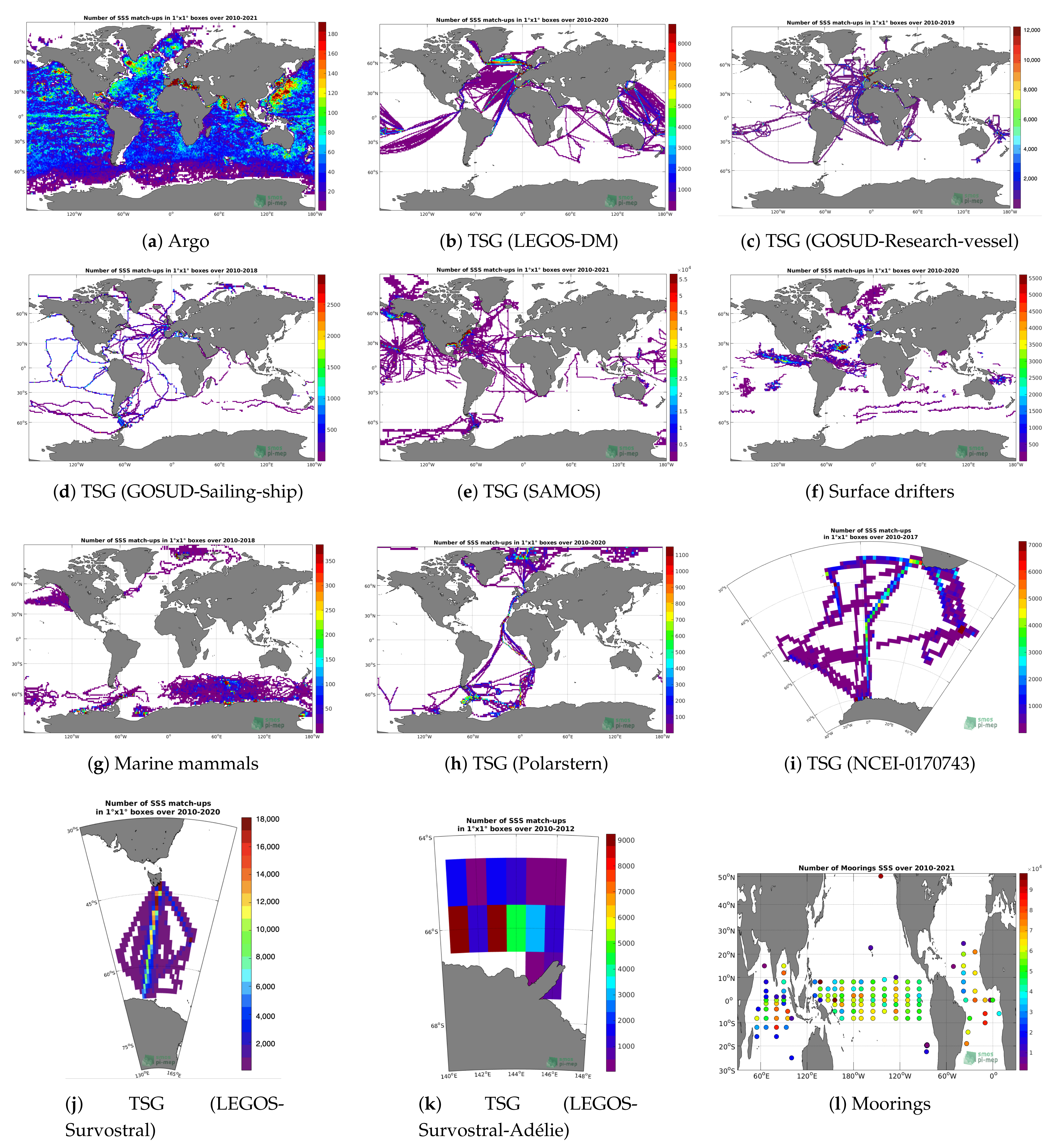

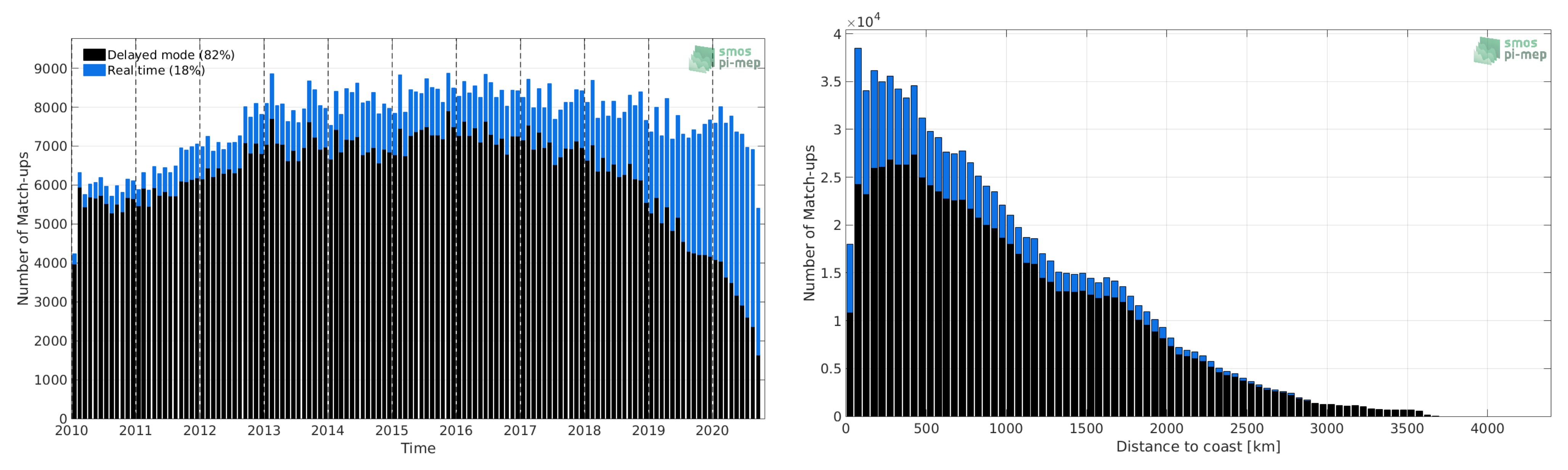
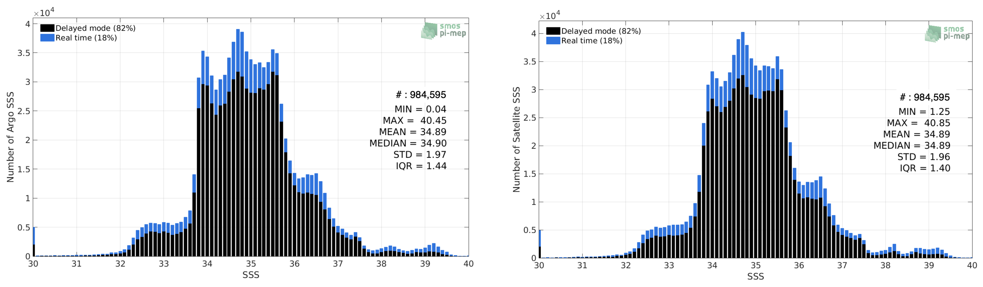
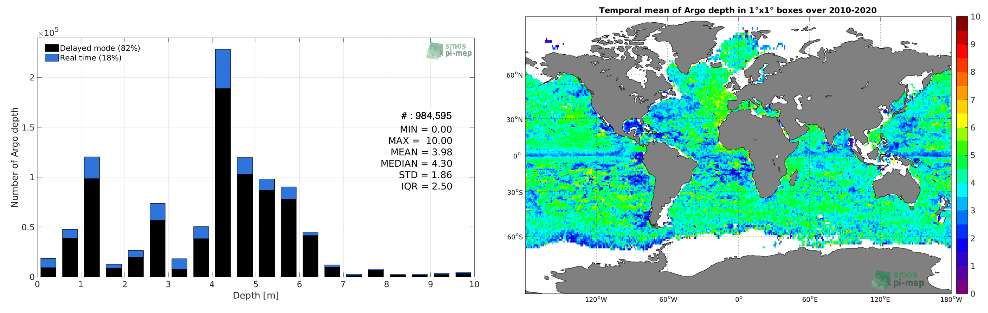
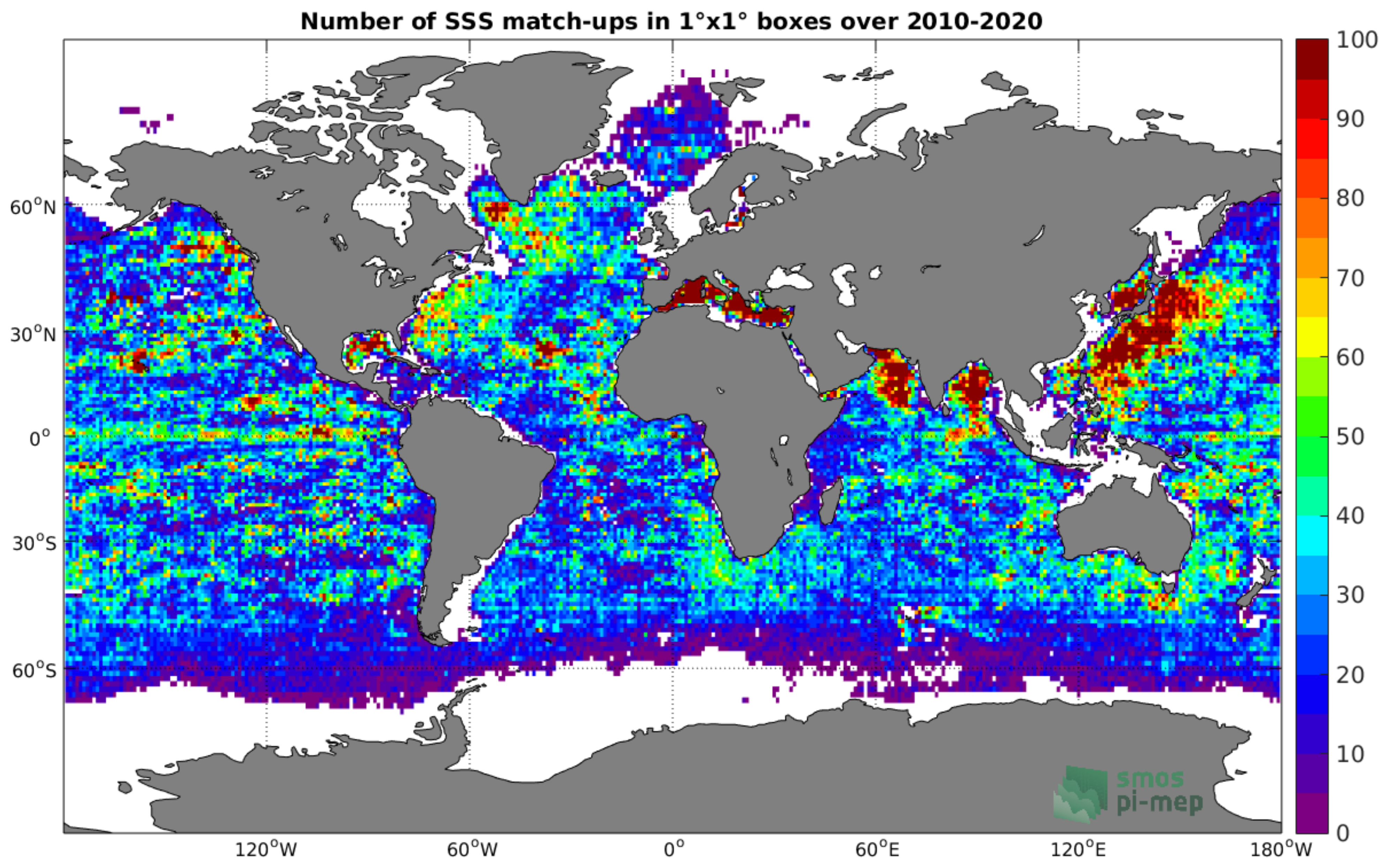
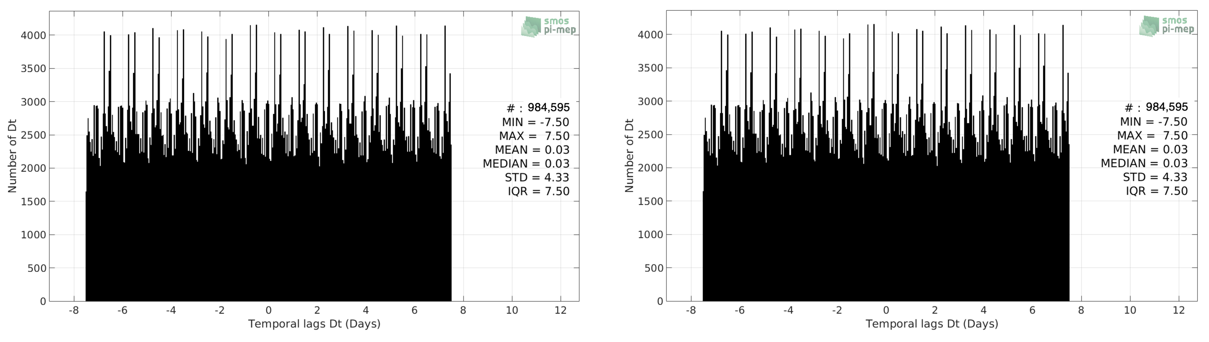
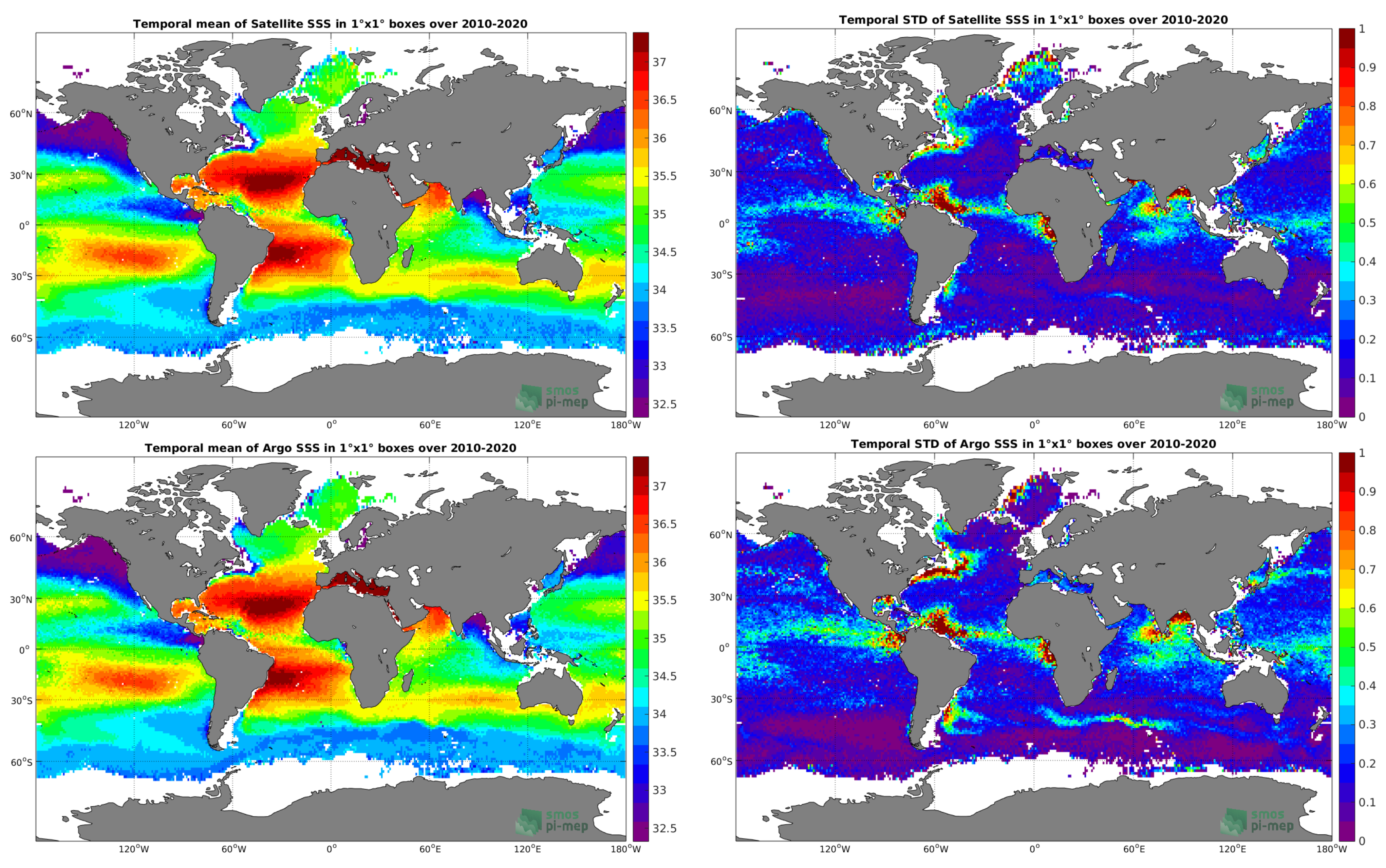
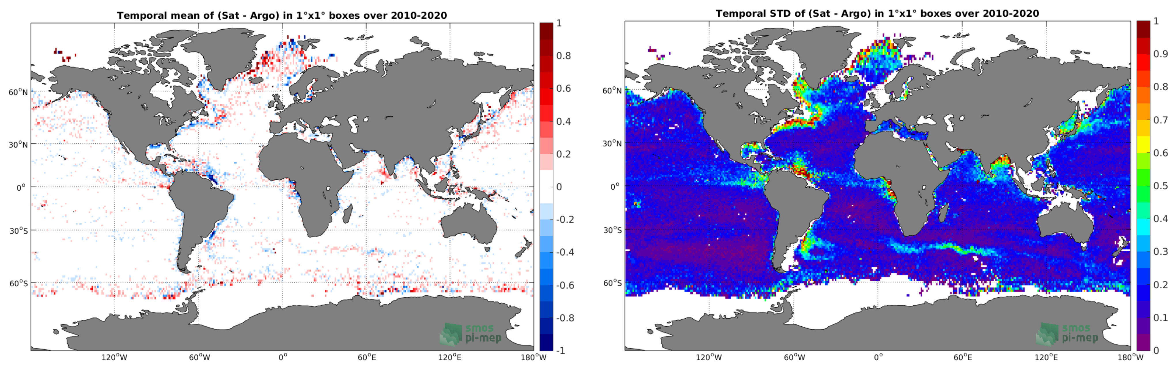

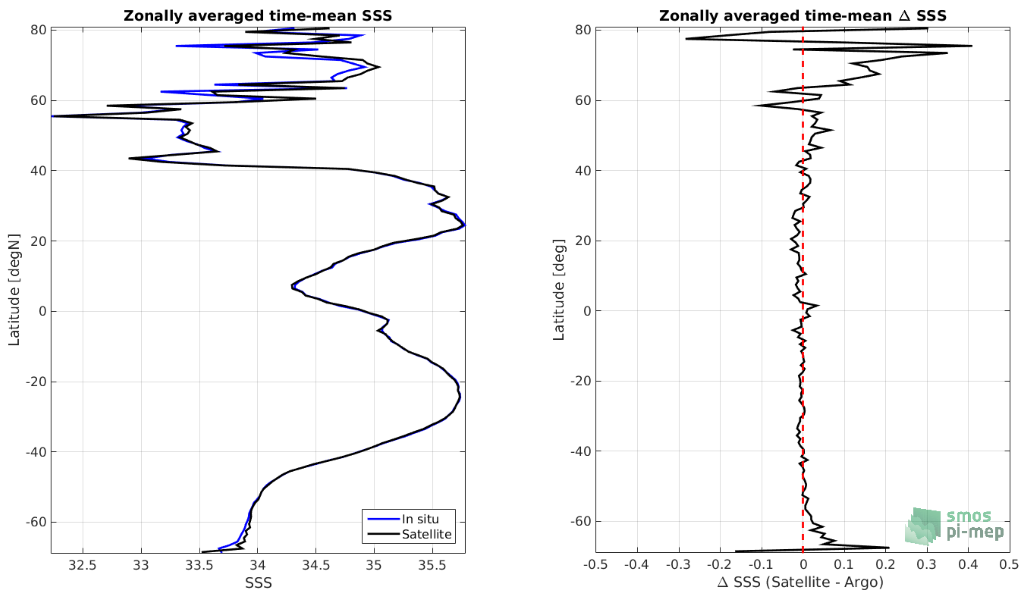
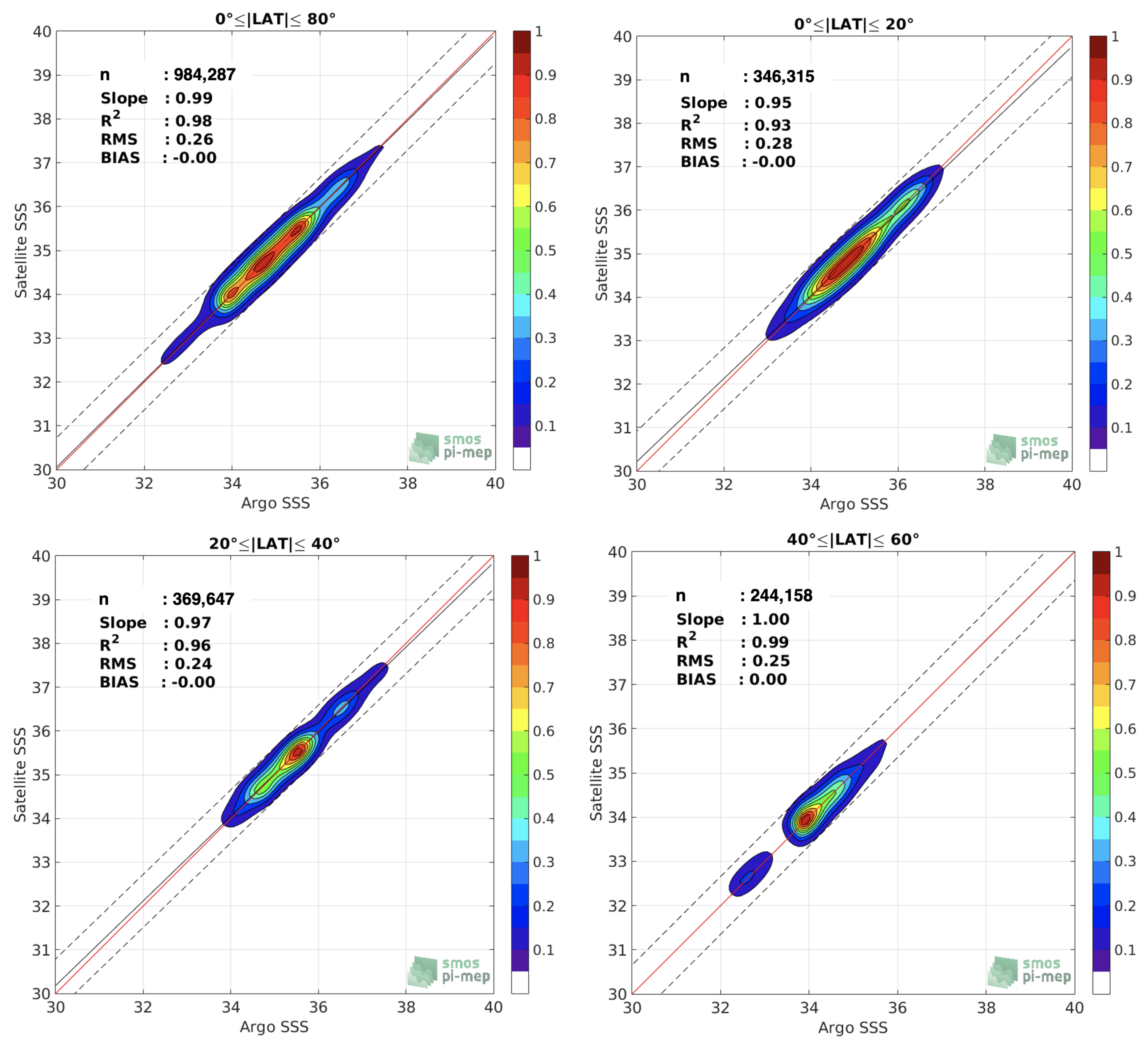
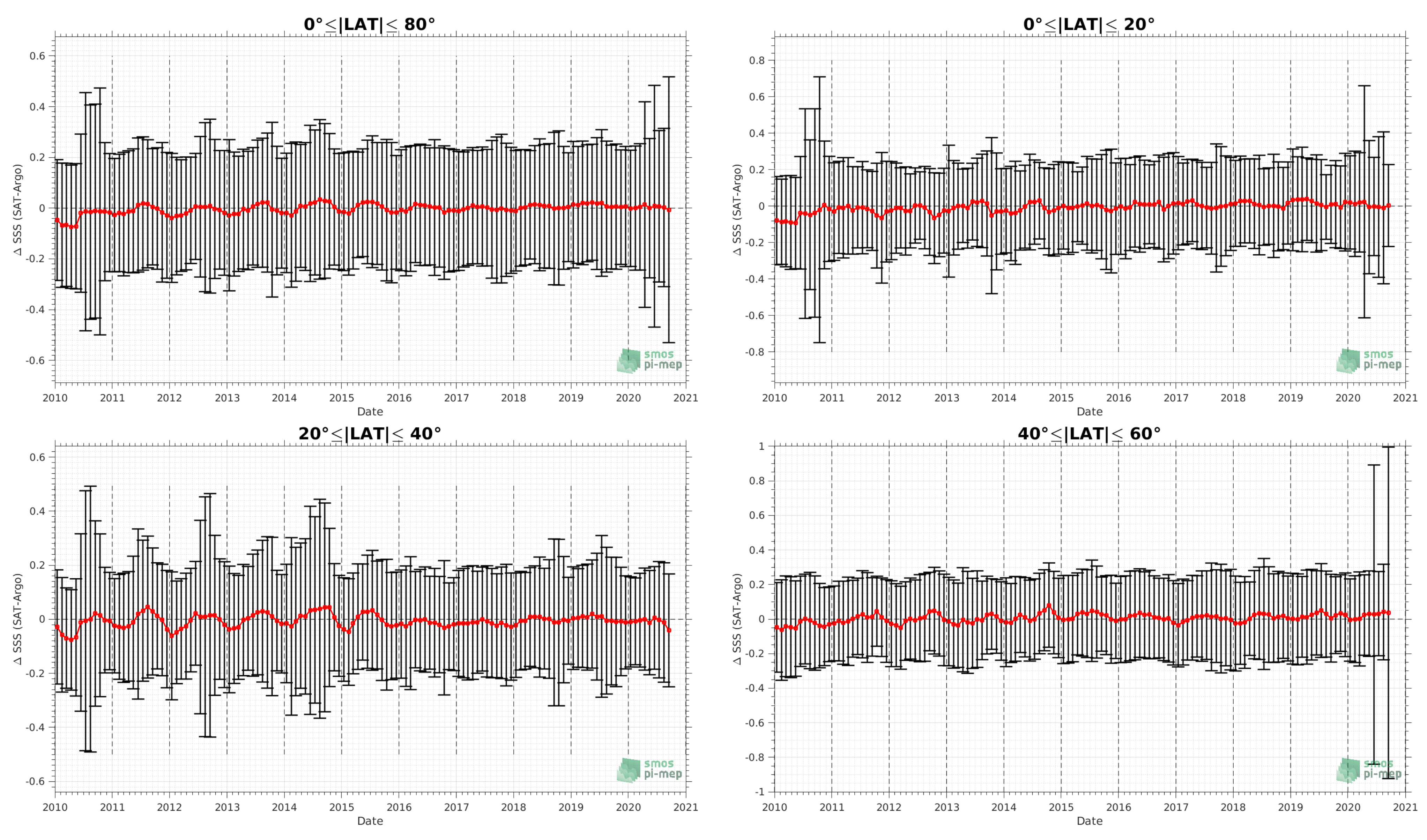
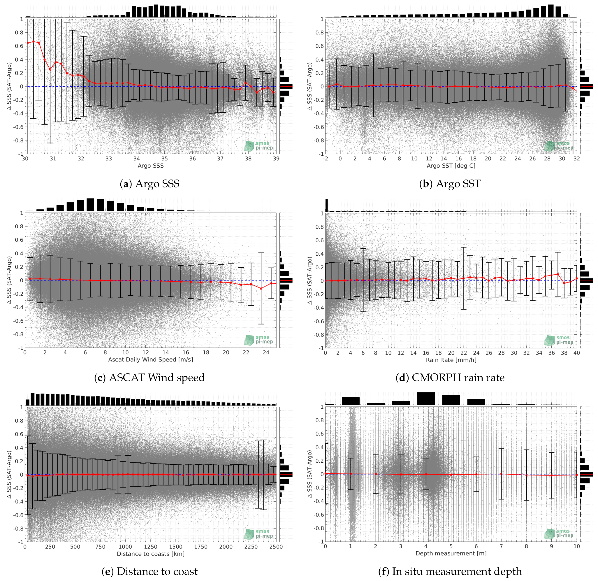

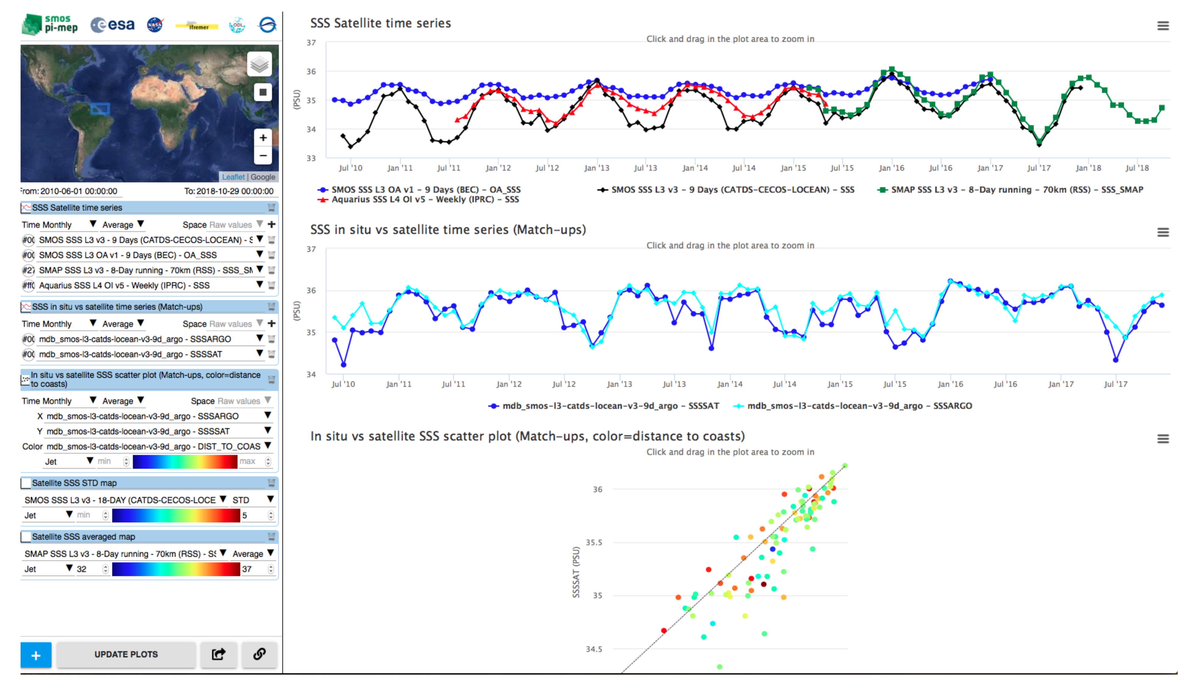
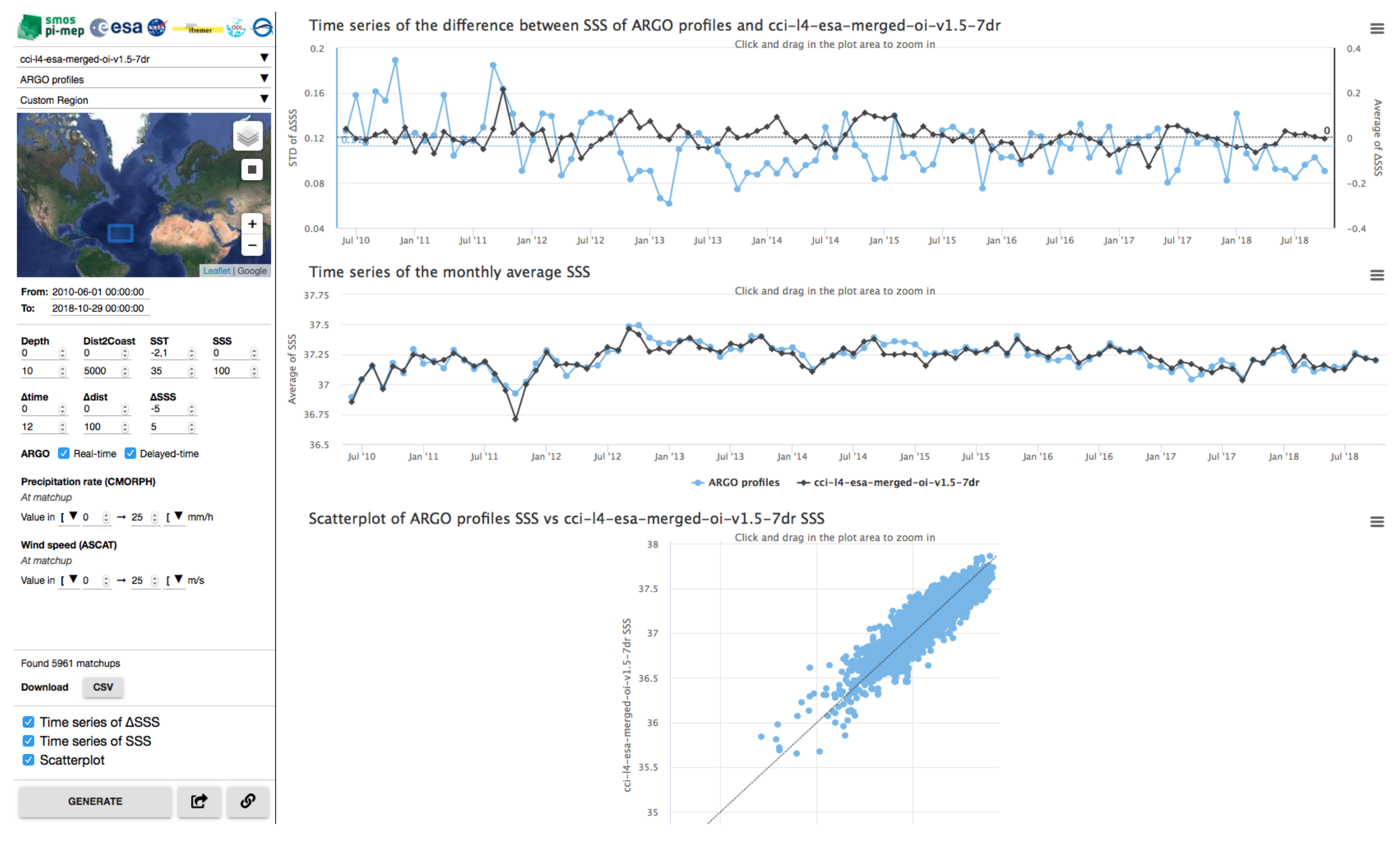
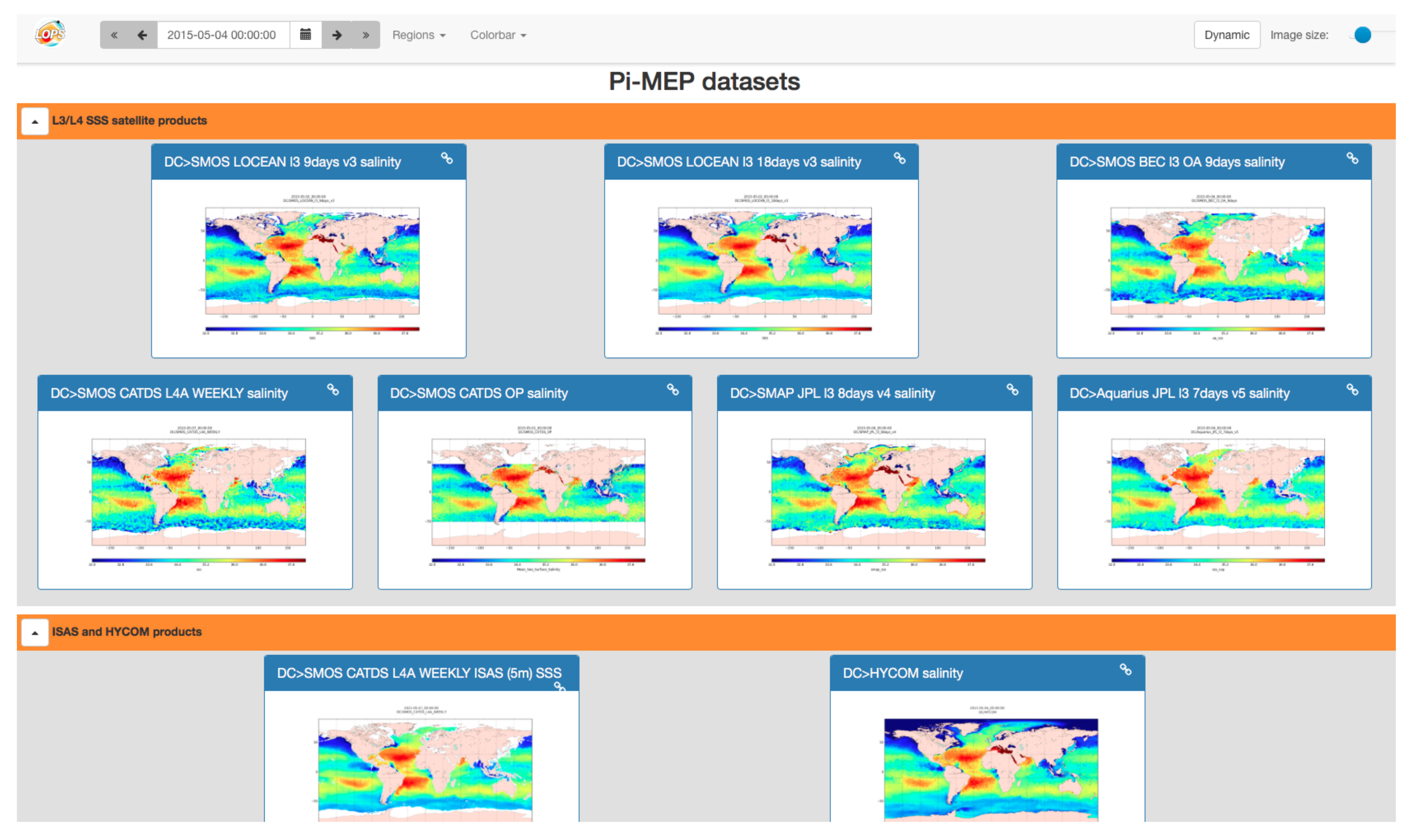

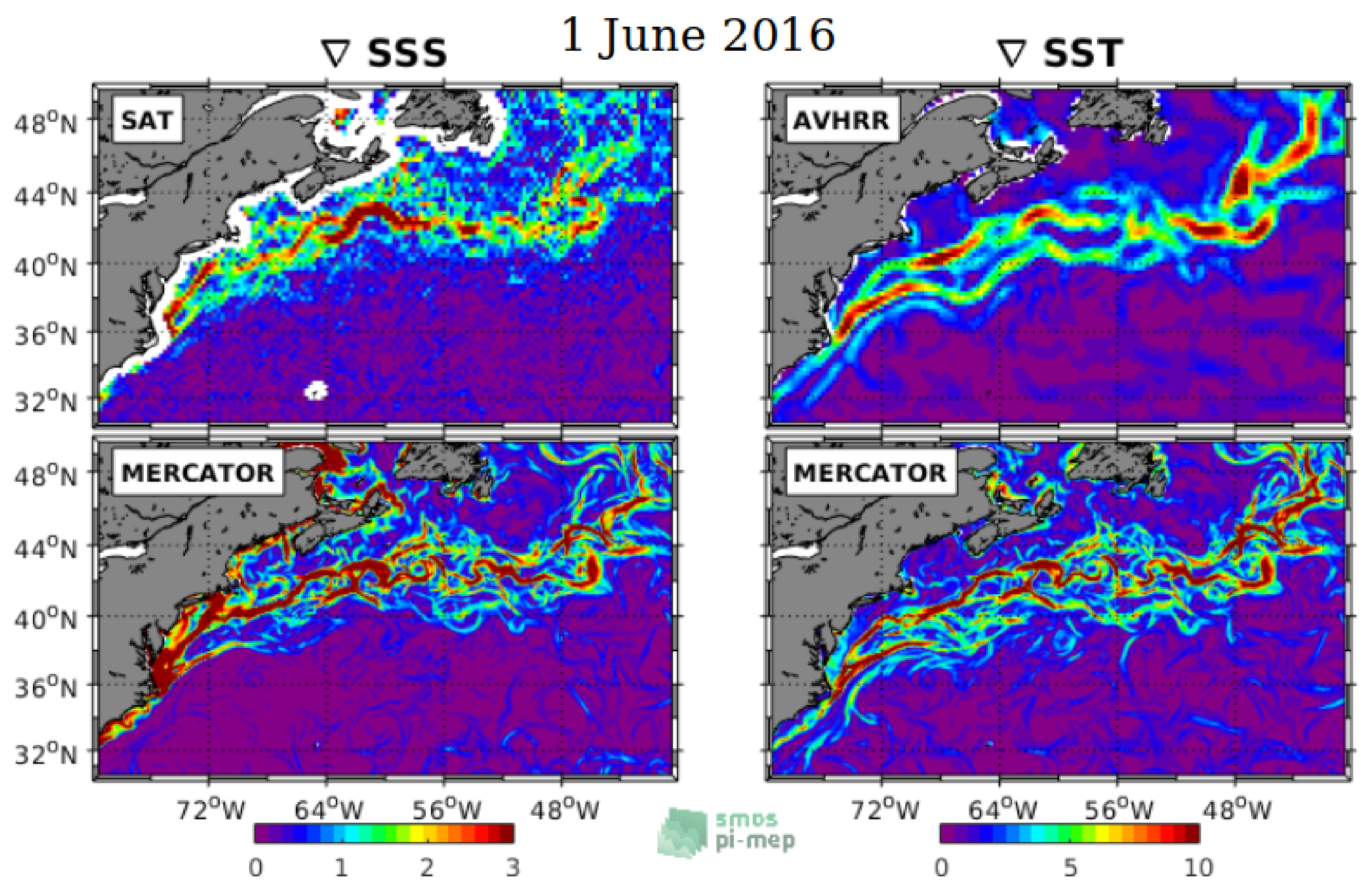

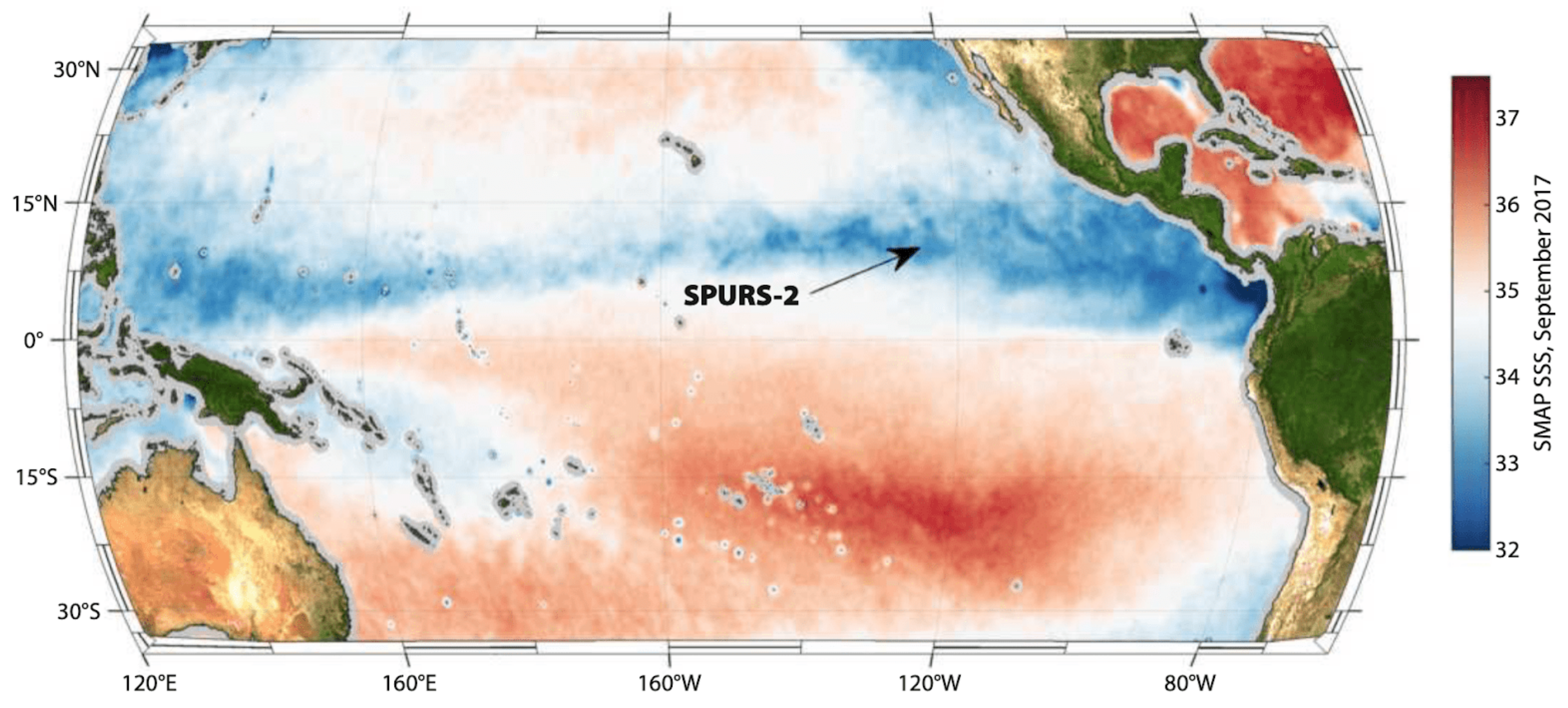
Publisher’s Note: MDPI stays neutral with regard to jurisdictional claims in published maps and institutional affiliations. |
© 2021 by the authors. Licensee MDPI, Basel, Switzerland. This article is an open access article distributed under the terms and conditions of the Creative Commons Attribution (CC BY) license (https://creativecommons.org/licenses/by/4.0/).