Communication

Landsat 8 Data as a Source of High Resolution Sea Surface Temperature Maps in the Baltic Sea

by
Katarzyna Bradtke
Institute of Oceanography, University of Gdańsk, Marszałka Piłsudskiego 46, 81-378 Gdynia, Poland
Remote Sens. 2021, 13(22), 4619; https://doi.org/10.3390/rs13224619
Submission received: 10 September 2021 / Revised: 10 November 2021 / Accepted: 12 November 2021 / Published: 17 November 2021
(This article belongs to the Special Issue Baltic Sea Remote Sensing)

Abstract

:
Sea surface temperature (SST) is a key hydrological variable which can be monitored via satellite. One source of thermal data with a spatial resolution high enough to study sub-mesoscale processes in coastal waters may be the Landsat mission. The Thermal Infrared Sensor on board Landsat 8 collects data in two bands, which allows for the use of the well-known nonlinear split-window formula to estimate SST (NLSST) using top-of-the-atmosphere (TOA) brightness temperature. To calibrate its coefficients a significant number of matchup points are required, representing a wide range of atmospheric conditions. In this study over 1200 granules of satellite data and 12 time series of in situ measurements from buoys and platforms operating in the Baltic Sea over a period of more than 6 years were used to select matchup points, derive NLSST coefficients and evaluate the results. To filter out pixels contaminated by clouds, ice or land influences, the IdePix algorithm was used with Quality Assessment Band and additional test of the adjacent pixels. Various combinations of flags were tested. The results show that the NLSST coefficients derived previously for coastal areas, characterised by a more humid atmosphere, might overestimate low SST values. Formulas derived for the Baltic Sea produced biases close to 0 °C and RMSEs in the range of 0.49–0.52 °C.

1. Introduction

The Baltic Sea is a semi-enclosed basin with a limited exchange of waters with the ocean. The general pattern of the spatial distribution of sea surface temperature is governed by the meridian extension of the sea and changes in bathymetry. However, surface temperature is highly variable over time, due to influence of large-scale atmospheric processes and the proximity of the land [1,2,3,4]. In the coastal zone, it might be modified by freshwater inflow, which is responsible for the brackish nature of the sea. Moreover, the heterogeneity of the coastline and bottom topography favour many locations of coastal upwelling, complex circulation and the formation of sub-mesoscale eddies, which play an important role in horizontal and vertical mixing [2,5,6]. The significant influence of coastal processes stems from the extent of the coastal zones which are relatively large compared to the sea area due to the elongated shape of the basin and numerous islands [2]. The resulting spatial inhomogeneity of the sea surface temperature (Figure 1) and the presence of thermal fronts affect the sea–atmosphere interactions, the weather conditions in the coastal zone, the functioning of ecosystems, fishing and tourism. Knowledge of the spatial and temporal variability of SST is crucial for weather forecasting, monitoring of the phenomena in the sea and supporting maritime services [7]. The boundaries between water masses which can be seen on the temperature maps may be a good indicator of the location of fronts and the directions in which the land substances responsible for eutrophication are moving. In the Baltic Sea high water temperature in summer is one of the factors contributing to cyanobacterial blooms [8] which in turn may increase the temperature locally due to the presence of surface scum and high concentrations of optically active substances [9,10,11,12].
In recent decades, numerous satellite systems have been developed for sea surface temperature mapping [7,14]. There is a growing body of literature showing their application in studies of the Baltic Sea (e.g., [1,4,5,6,13,15,16]) and in operational modelling, as a source of data for assimilation (e.g., [13,17,18]). Comparisons of satellite-derived SSTs with in situ bulk temperatures measured in the Baltic Sea yielded root mean square errors (RMSE) in the range of 0.5–1.3 °C [1,4,6,13,16,19,20]. The highest errors are usually attributed to imperfections in the cloud screening algorithms. Satellites equipped with infrared (IR) radiometers (e.g., AVHRR, MODIS, VIIRS, SLSTR or SEVIRI), commonly used for SST mapping in these studies, provide information with high temporal resolution in near-real-time mode. However, their spatial resolution (0.75–4.8 km at nadir) might be too coarse to observe sub-mesoscale processes in coastal regions [7]. To derive SSTs in such areas, higher-resolution IR radiometers, designed to observe the surface of land, may be used [14]. From the radiometers currently operating and providing IR data for the Baltic Sea, these are the Enhanced Thematic Mapper (ETM+) and Thermal Infrared Sensor (TIRS) on the Landsat 7 and 8 satellites, respectively, and the Advanced Spaceborne Thermal Emission and Reflection Radiometer (ASTER) on the Terra satellite; the others do not cover the Baltic Sea area. The aforementioned instruments record IR data with a spatial resolution of 60–100 m. The Landsat mission satellites provide IR data on a regular basis from daytime observations (descending mode) and 185 km wide swath. The ASTER radiometer does not collect data continuously; they are gathered only for selected areas of 60 × 60 km, as requested by authorised ASTER users. Thanks to the long duration of the Terra mission, many scenes were also collected for the Baltic Sea but with a revisit time of months. Landsat satellites have a 16 day repeat cycle, though the large overlap between scenes in the mid-latitudes results in a 5–8-day revisit time for similar areas in the Baltic Sea [21].
The Landsat mission is run by the Earth Observation Program of the National Aeronautics and Space Administration (NASA). Data processing and quality control is ensured by the U.S. Geological Survey (USGS), which provides a consistent archive (Collection) of Landsat data reprocessed according to a common algorithm to support time series analysis. Launched in 2013, Landsat 8 carries a Thermal Infrared Sensor (TIRS) with two infrared channels (band 10 and band 11 centred at 11 µm and 12 µm, respectively) collecting data of 100-m resolution [22]. This allows for split-window algorithms that use a two-channel approach to correct the influence of the atmosphere. TIRS has undergone significant improvement over previous Landsat missions, which were equipped with single thermal infrared band sensors (TM or ETM+). The second instrument carried by Landsat 8, an Operational Land Imager (OLI), collects data in the visible (VIS), near-infrared (NIR) and short-wave infrared (SWIR) portions of the spectrum, which facilitates the identification of clouds. Although a high spatial resolution is achieved at the expense of reduced swath width and temporal resolution, existing research shows that TIRS data provide useful SST information for studying sub-mesoscale phenomena [23], land–sea interactions [24,25], coastal water quality [26,27] and ecosystem management [28,29]. An intercomparison of SSTs derived from Landsat and lower resolution radiometers can also help to understand variability within a satellite pixel and differences between satellite and in situ data [7]. Due to the patchy nature of cyanobacterial blooms, the high spatial resolution of SST adds value to the study of the relationship between SST and the occurrence of blooms [12]. Given the challenges of expanding operational modelling capabilities in the Baltic Sea, from the basin scale to the local coastal-estuarine scale [30], Landsat data may also be useful as auxiliary data for assimilation.
Despite the potentially wide range of applications, no SST algorithm for Landsat 8 has been verified globally or locally for many regions, including the Baltic Sea. This certainly limits the current use of these data in oceanographic research. Several attempts have been made to establish a Landsat 8 TIRS algorithm for retrieving SST maps. Most studies have only focussed on single-channel algorithms [23,28,31,32,33] due to the calibration uncertainties in TIRS band 11 (~12 µm) associated with stray light issues [34]. Several researchers have proposed correction of the brightness temperature band 10 (~11 µm) using SSTs estimated from other satellites’ simultaneous recordings [23,28] or measured in situ [31,32]. Unfortunately, most of these works used only individual Landsat scenes; a wider assessment of SSTs was only presented by the authors of [28]. They showed that SSTs may be retrieved using the TIRS brightness temperature at a single channel and atmospherically corrected NOAA AVHRR data with an RMSE of 0.82 °C, calculated with respect to in situ data from buoys. A different approach based on the radiative transfer model has been proposed by [33] with an RMSE of 0.7 °C in cloud-free conditions or 1.0 °C for images with scattered clouds. However, this approach requires auxiliary data on the atmospheric profiles of relative humidity and temperature.
A solution that is less dependent on additional data sources is the split-window algorithms that use the difference between the brightness temperature in both TIR channels to determine the water vapour content in the atmosphere. The use of TIRS band 11 is no longer limited since stray light correction was implemented and uncertainties were reduced starting with Landsat Collection 1, distributed by the USGS since 2017 [35]. The authors of [36] have used the data from this collection and in situ observations to determine the split-window algorithm coefficients and to evaluate its accuracy based on a sufficiently large number of comparisons with in situ data from coastal waters around the Korean Peninsula. Other attempts were only based on a small number of Landsat 8 matchup points and/or applied to a very narrow range of temperatures and atmospheric conditions [27,29,32,37]. Jang and Park [36] showed that SSTs may be retrieved using the nonlinear SST formula (NLSST) with empirically determined best fit coefficients with RMSE in the range of 0.59–0.66 °C, depending on the source of the first guess of SSTs and whether the satellite zenith angle is considered or neglected. They stated that the NLSST coefficients derived in their study might be applicable for other coastal regions of the global ocean.
The NLSST formula was developed by [38] and has commonly been used in the past few decades for NOAA AVHRR [13,19,39,40]. The main limitation of this formula is the fact that the relationship between the attenuation of IR radiation in the atmosphere and the temperature difference in the two TIR channels depends on a water vapour regime [40,41]. In the Baltic Sea, during the warm season (May–September) the sea surface temperature often drops locally below 10 °C due to coastal upwelling, which affects the distribution of water vapour in the lower layer of the atmosphere. The temperature difference between the two TIR channels is greatly reduced under such conditions [41]. The authors of [36] found that their algorithm tends to overestimate SST if the split window difference is lower than 0.5 °C. Thus, the algorithm coefficients may need to be adjusted for use in the Baltic Sea. An additional adjustment may also be necessary due to an improved radiometric calibration applied to Collection 2 products, currently reprocessed and provided by the USGS [42].
The main goal of this work was to calibrate the NLSST algorithm for use in the Baltic Sea with Landsat 8 data to derive high-resolution SST maps and to assess how the improved radiometric correction applied to TIRS data influences the estimation of SST. The main motivation to address these problems was the fact that the potential of the TIRS sensor in the Baltic region has not been utilised so far. To facilitate the use of this data by a wide group of oceanographers, the analysis was focussed on algorithm that do not require auxiliary data from other sources and can be implemented using the freely available tools or services.

2. Materials and Methods

2.1. Data

Satellite data gathered by Landsat 8 between March 2013 and July 2019 over the Baltic Sea were analysed. Level 1 data from USGS OLI/TIRS Collection 2 were downloaded using the USGS Earth Explorer Service (https://earthexplorer.usgs.gov/; accessed on 1 March 2021). Only granules with cloud cover not exceeding 60% and covering positions in the reference in situ data were considered (Figure 2).
A standard Level 1 USGS product includes orthorectified and gridded TOA radiances for all OLI and TIRS spectral bands, coded into integer digital numbers, quality band (QA Pixel) with assessment flags for each pixel, and angle coefficients and product metadata files. To assess the impact of the newest radiometric calibration on SST estimation and to assess the efficiency of contaminated pixels filtering, L1 TIRS data from Collection 1 were also ordered and downloaded via EROS Science Processing Architecture On Demand Interface (ESPA USGS; https://espa.cr.usgs.gov/; accessed on 1 March 2021).
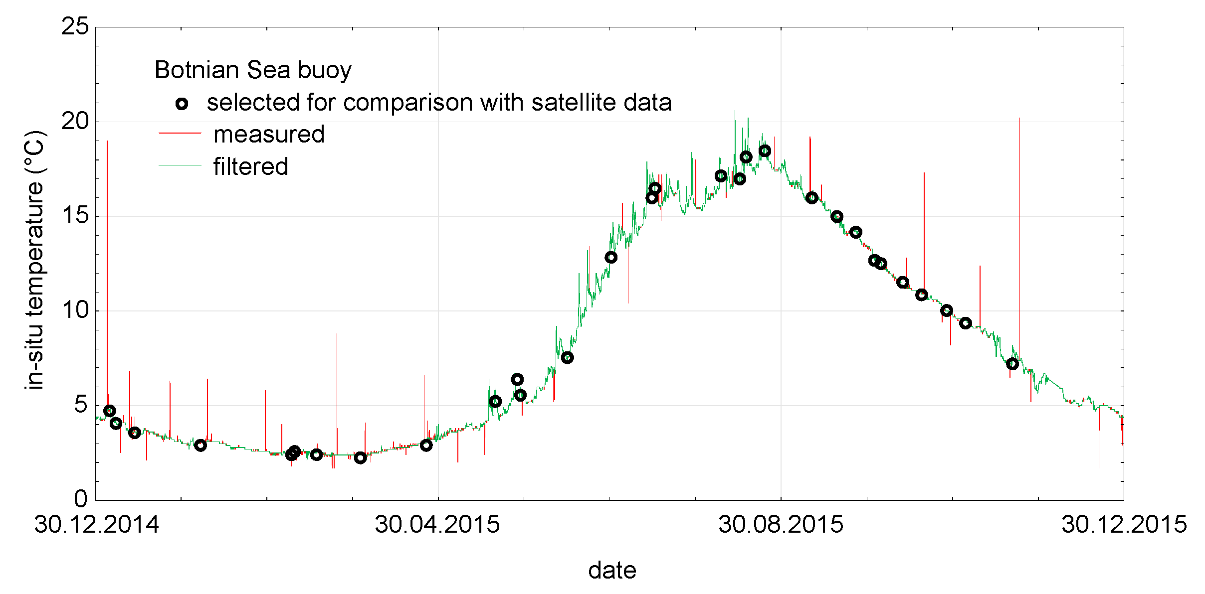
In order to validate the satellite-derived SST, in situ data provided by buoys or monitoring stations operating on the Baltic Sea within the framework of the Baltic Operational Oceanographic System (http://www.boos.org/ accessed on 1 March 2021) were used. Nine buoys and three platforms (Table 1, Figure 2) were selected, taking into account the length of time series covering the period in question and their locations at different distances from land and in different basins. Datasets were gathered from Copernicus Marine Service (INSITU_BAL_NRT_OBSERVATIONS_013_032 product, MO datatype). All observations from different platforms are aggregated by the In Situ Thematic Centre and provided to users after quality control [43]. Only temperatures with the quality flag “good data” (QC = 1) measured at the first depth level (in the 0 to 0.5 m layer) were included in the study. Despite the filtering of data in terms of quality, some of the time series were contaminated with outliers (the most contaminated ones were the Bothnian Sea and the Northern Baltic data). Thus, prior to further analysis, the time series were additionally cleaned using the Hampel filter [44] with a 24 h moving window (Figure 3).
Prior to the satellite data processing steps, the matchup procedure was done taking into account the time of scene acquisition and in-situ measurements. The granule was further processed if there was a reference measurement taken within half an hour of the scene acquisition and if the pixel containing the location of the measurement was valid (contained TOA L1 data for all spectral bands). In total, 1213 matchup points were found by taking only the most recent reference data for each pixel. The number of processed Landsat 8 scenes was 1046, all with a scene quality score of 9 (best). All of them were gathered during descending mode (acquisition time between 9:20 and 10:30 GMT).

2.2. NLSST Formula

To derive SST from the TIRS infrared bands, a nonlinear algorithm (NLSST) was used as proposed by [38] and utilised for Landsat 8 by [36]:
SST = a1T11 + a2(T11 − T12)Tclim + a3(T11 − T12)(secθsat − 1) + a4,
where
Tclim ~ MCSST = b1T11 + b2(T11 − T12) + b3(T11 − T12)(secθsat − 1) + b4,
SST is the sea surface temperature in °C; T11, T12 are the brightness temperature in K in the TIRS bands centred at ~11 µm and ~12 µm, respectively, θsat is the satellite zenith angle, Tclim is a first guess for SST or the climatological SST value in °C and a1-a4 and b1-b4 are the best-fit coefficients.
The SST first guess in Equation (1) can be estimated by the multichannel formula (MCSST) used in this study or it can be obtained from any other SST source, for example, climatological SST data records. Digital numbers from the TIRS bands were converted into brightness temperatures according to standard USGS procedure [22] using the calibration coefficients included in the metadata files. The satellite zenith angle for each pixel was calculated using the Solar Illumination and Sensor Viewing Angle Band Tool [45] and the angle coefficients file. Due to the along-track distribution of TIRS detectors, the viewing angles are slightly different for each spectral band. Thus, the average values were calculated for both TIRS bands.
The assessment of SST estimation was performed with the standard parametric measures: systematic error (bias) and RMSE defined as the average and standard deviation of SST residuals, respectively. The determination coefficient (r2) for the relationship of estimated SST vs reference temperature was used as well.
SST residuals (ΔSST), defined as difference between the satellite-derived sea surface temperature (SST) and the reference in situ bulk temperature (T), represent errors originating from cloud contamination, insufficient correction of radiation attenuation in the atmosphere or diurnal warming of the surface layer. Even though the NLSST coefficients are calibrated based on the bulk temperature measurements, IR emission and thus the brightness temperature from the satellite only respond to a thin surface layer, where diurnal warming is much more pronounced than at depths where the bulk temperature is measured. This is especially true for Landsat data that are recorded during the daytime.

2.3. Cloud and Ice Masking

To exclude erroneous pixels, contaminated by clouds, ice or land, the pixel quality assessment band (QA Pixel) provided by USGS was used. The flags included in this product are based on the CFMask algorithm [22] which utilises decision trees and a multi-pass approach [46]. The L1 processing creates flags of confidence (“high”, “medium” or “low”) for clouds, cloud shadows, cirrus and snow/ice. The cloud confidence flags are further processed into a cloud mask, a dilated cloud mask and an additional flag indicating “water” pixels [47]. The QA Pixel band flags are consistent with those included in the Level 2 pixel quality assurance band for Collection 1 products (BQA L2).
Only pixels over water, with low confidence of clouds, ice and cirrus which were not indicated as “dilated cloud”, were considered initially as “clear”. The initial mask that excludes all other pixels is hereafter referred to as QA mask. To improve the masking of contaminated pixels, the IdePix Landsat 8 OLI processor product was additionally tested. This processor is implemented in Sentinel Application Platform (SNAP), an open-source common architecture for ESA Toolboxes for the exploitation of Earth Observation data (http://step.esa.int/main/toolboxes/snap/; accessed on 1 March 2021). The IdePix classification algorithm was developed by Brockmann Consult GmbH (https://www.brockmann-consult.de/portfolio/idepix/; accessed on 1 March 2021) and is based on a neural network approach. In this study, version 8.0.0 was run with the standard neural net applicable for most conditions. This processor classifies pixels as certainly or ambiguously being affected by clouds, cloud shadows or snow/ice. The final cloud mask includes only “cloudy for sure” pixels. An additional step provides the flags “white” and “bright” based on reflectance from the OLI RED (4) and NIR (5) channels (over water). The latter also included pixels flagged as “cloud for sure”.
The effectiveness of masking to reduce negative outliers was assessed on the basis of SST residuals, and a visual assessment of the spatial and temporal distribution of SSTs. To calculate SST, the values given by [36]—a1 = 0.9026, a2 = 0.0802, a3 = 32.0333, a4 = −245.14619, b1 = 0.9742, b2 = 1.7742, b3 = 32.9868 and b4 = −266.03903—were taken as a first approximation of the coefficients ai and bi in the NLSST formula applied to Collection 1 TIRS data.

2.4. SST Algorithm Calibration

The most efficient combination of flags was used to eliminate contaminated pixels from the matchup dataset prior to further analysis. In order to adjust the coefficients of SST Equations (1) and (2), a non-linear regression was applied to a randomly selected training subset of data. The analysis was carried out for two versions of the NLSST algorithm: full (NLSST v1), taking into account the satellite’s zenith angle, and simplified (NLSST v2), omitting the third term of Equations (1) and (2). The simplification results from the relatively narrow Landsat viewing angle with respect to nadir, which is in the range of approximately ±8.5° (secθsat ≅ 1).
To limit the impact of outliers on regression results, the SST residuals previously calculated using the NLSST algorithm proposed by [36] were used to detect outlying cases. They were omitted when dividing the data into the training (75%) and test (25%) subsets. Outliers were defined as cases with residuals ΔSST greater than Q3 + 1.5 × IQR (positive outliers) or less than Q1 − 1.5 × IQR (negative outliers), where Q1, Q3 and IQR represent the lower quartile, upper quartile and interquartile range, respectively.

3. Results

3.1. Improvement of Contaminated Pixel Masking

For the first overall assessment of SST derived from Landsat 8 data, only pixels classified on the base of CFMask flags as initially “clear” (free of cloud, cirrus, ice and land contamination) were included (n = 790). The calculated RMSE was relatively high (1.31 °C), but as shown in the scatterplot and in the distribution of residuals in Figure 4, most of the SST values were in good accordance with in situ measurements. Estimated SSTs were in the range of −3.4–25.3 °C and reference temperatures in the range of 0–25.5 °C. An average temperature with the standard deviation was 10.84 °C ± 6.13 °C and 10.92 °C ± 6.12 °C, respectively. The high RMSE resulted mainly from insufficient masking of contaminated pixels.
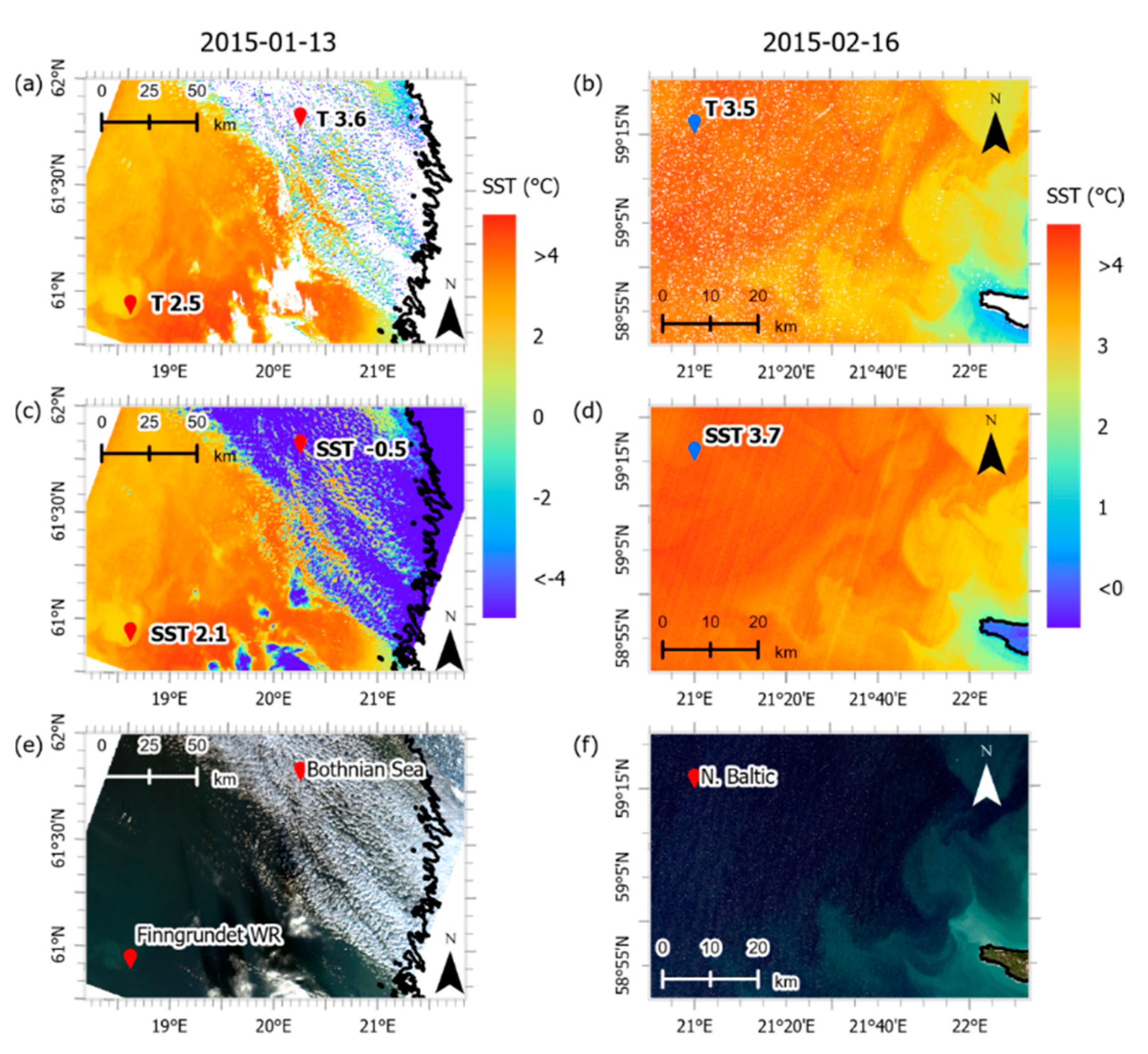
Two flags, “ambiguous” clouds and “bright” pixels, were selected from the IdePix product to extend initial QA mask. The flag “bright” also included sparse pixels flagged as “cloud for sure” (Idepix cloud mask). The IdePix flag “white” was not considered as this flag was set for a considerable number of appropriate pixels. By further filtering out matchups with the flags: “ambiguous clouds” and/or “bright” the RMSE was reduced to 0.91 °C (Figure 5a). Unfortunately, single cases with errors of underestimating the temperature even by more than 3.5 °C still existed. A visual inspection of the SST maps revealed that these errors were related to pixels near the boundary of the mask (Figure 6a). To solve this problem, a buffer of 100 m around mask was applied (Figure 5b). However, it was noted that the IdePix “ambiguous clouds” flag was sensitive to the increase in reflectance noted for many individual pixels or small groups of pixels when surface blooms, aerosols in the atmosphere, direct reflections from a wavy surface or instrumental noise were present. In such cases, many isolated pixels—for which no changes in IR channel response were observed—were erroneously classified as ambiguous clouds (Figure 6b). The problem increased with the use of a buffer, which eliminated a significant percentage of the pixels where the SST was in good agreement with the in situ reference temperature (Figure 5b).
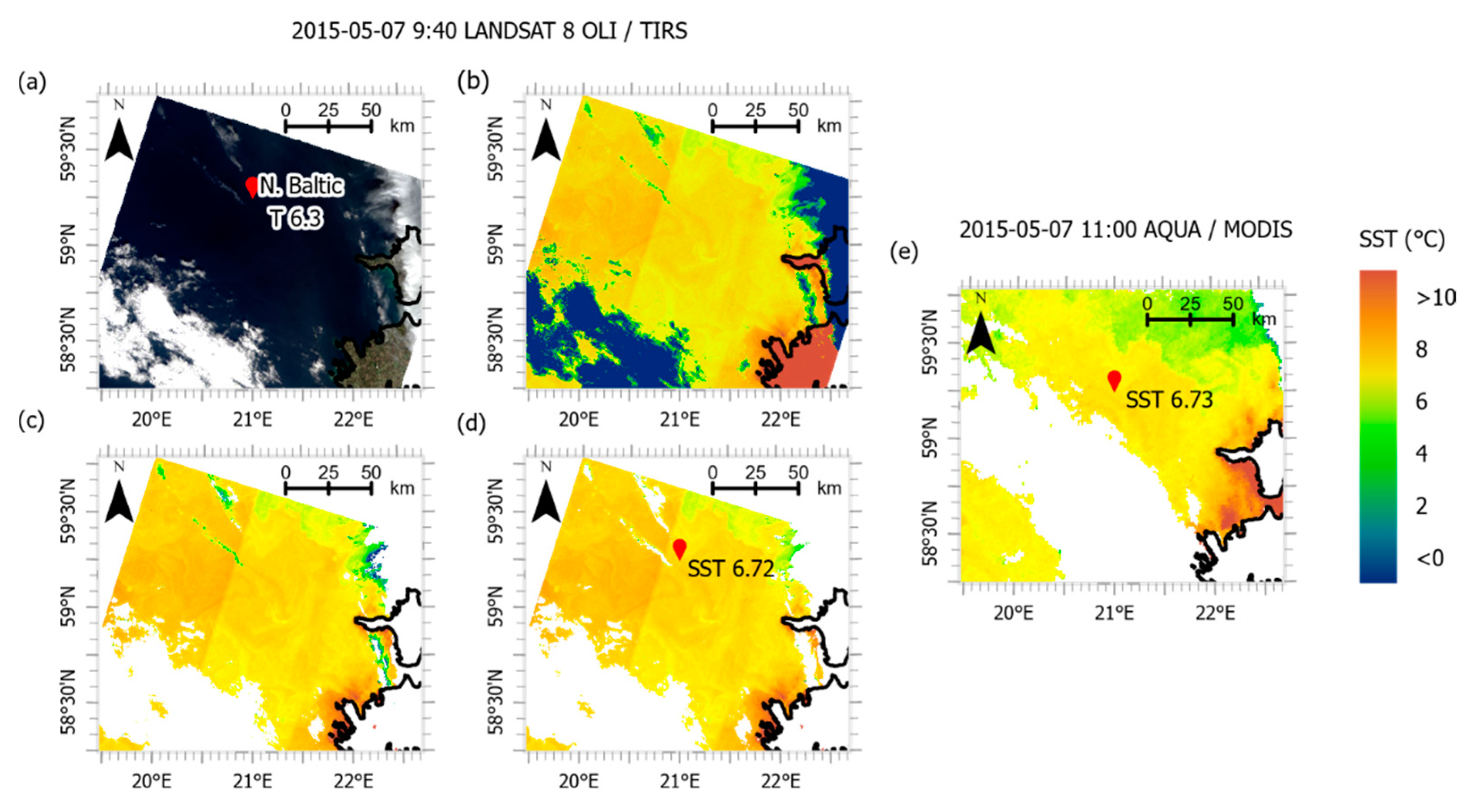
Therefore, an amendment to the masking procedure was proposed. Groups of adjacent pixels classified as “ambiguous cloud” were analysed in terms of their size. If they were composed of five pixels or less, the flag was reset to False. In the next step, the pixel groups considered to be valid were analysed. If the area enclosed by a mask was less than 1 km2, it was treated as a whole as contaminated border pixels and added to the mask. The mask, corrected this way, was further extended by a buffer of 100 m (Figure 5c). The final mask eliminated fewer appropriate pixels (SST residuals close to zero) than the one without correction, though both filtered out most of the highest negative outliers (Figure 5b,c). The buffer size resulted from the actual resolution of the TIRS channels. Figure 7 shows a comparison of initial and final masks’ performance for an example Landsat image. As can be seen in the upper-right corner of the map (Figure 7d), the buffer width should be extended to eliminate all pixels where clouds influence the SST; however, in other regions it would lead to over masking.

3.2. Calibration of the SST Equations

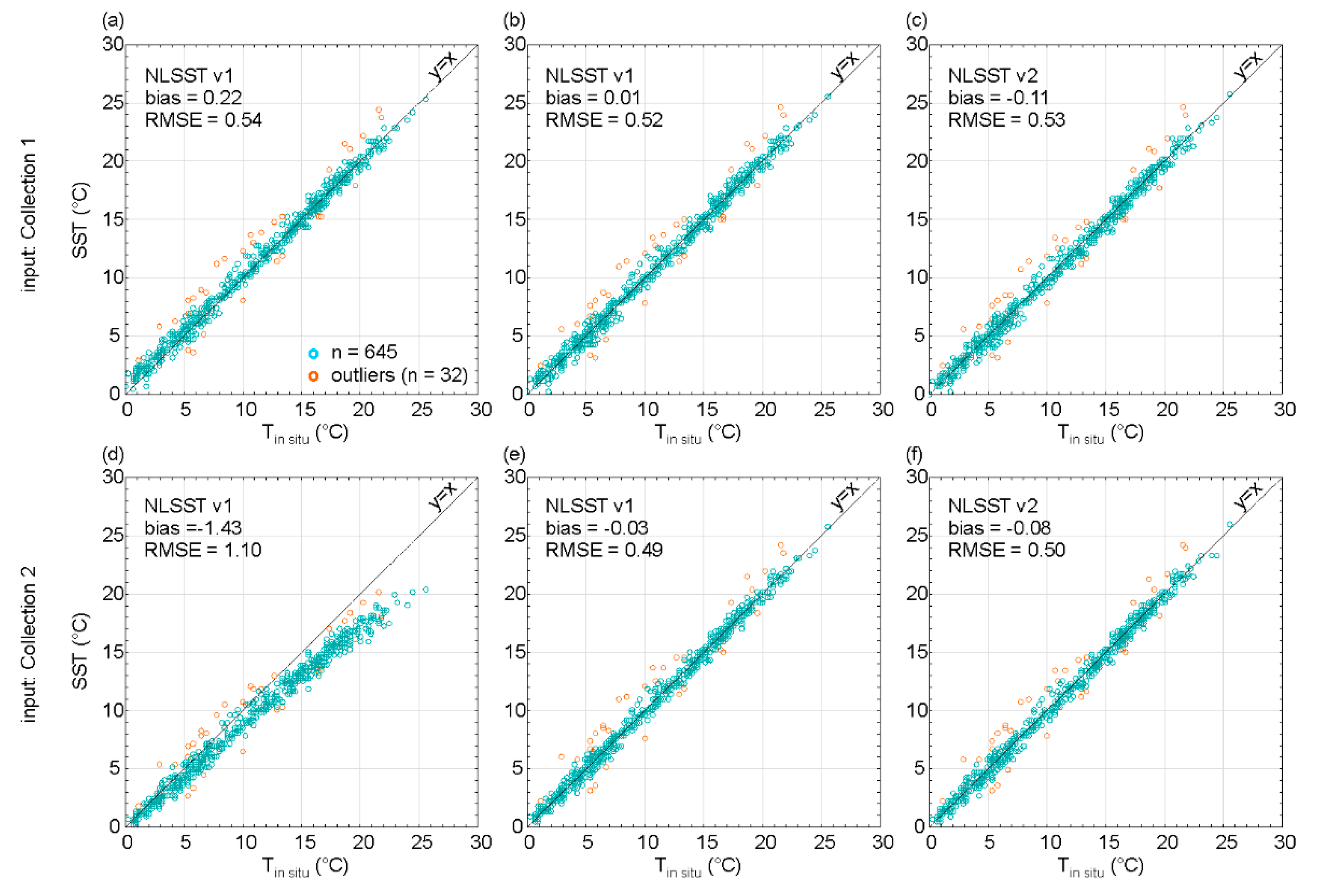
In order to adjust the NLSST coefficients, “clear” pixels were selected from the matchup dataset using the mask which was a combination of QA mask and the IdePix flags with additional corrections (Figure 5c). Of the selected 677 matchup points, 32 were outliers. The remaining cases were divided into a training (75%) and a test set (25%). The best-fit coefficients for both versions of the NLSST algorithm obtained from the training subset of matchups are listed in Table 2. Both Landsat data collections were considered an input to the regression analysis. The comparison of estimated SST with the in situ temperature is shown in Figure 8. The assessment of all sets of coefficients for the training and the test subsets of matchup points showed similar results, therefore bias and RMSE shown in Figure 8 were calculated for all data excluding outliers. For comparison, the NLSST algorithm with coefficients derived by [36] is also included (Figure 8a,d). In this case the same set of coefficients was applied for data from both collections.
The data from Collection 1 and the NLSST Equation with the coefficients given by [36] and fitted with Baltic Operational Oceanographic System data (NLSST v1 in Table 2) show similar accuracy with respect to RMSE (Figure 8a,b), which was 0.54 °C and 0.52 °C, respectively. However, the new set of coefficients improved the estimation of low SSTs that had previously been overestimated, in general. The bias decreased from about 0.2 °C (Figure 8a) to close to zero (Figure 8b) and the trend of residuals with respect to in situ temperature was reduced. The omission of the term with correction for the viewing angle (NLSST v2) only slightly modified the other coefficients, as compared to the full version (Table 2). The estimates of those coefficients for the NLSST v2 were generally within the confidence intervals (95% confidence level) of the coefficients determined for the NLSST v1, regardless of the data source (Table 2). However, the use of a simplified version of the algorithm more often resulted in underestimating the SSTs in relation to in situ data in the entire range of analysed temperatures (compare Figure 8b,e and Figure 8c,f, respectively). The bias for both data sources increased from close to 0 °C (NLSST v1) to −0.1 °C (NLSST v2). The RMSE remained almost unchanged.
The NLSST coefficients derived for the recalibrated data provided by the USGS Collection 2 differed significantly (higher difference than the standard error of estimation) compared to those derived for Collection 1 for both versions of the algorithm (Table 2). Surprisingly, only a slight reduction of the RMSE error to about 0.5 °C for both versions of the algorithm was obtained after using the recalibrated data provided by USGS Collection 2 and the coefficients adjusted to these data (compare Figure 8b,c and Figure 8e,f). It should be noted that coefficients derived for Collection 1 would lead to a significant underestimation of SST if applied for recently recalibrated data (compare Figure 8a,d).
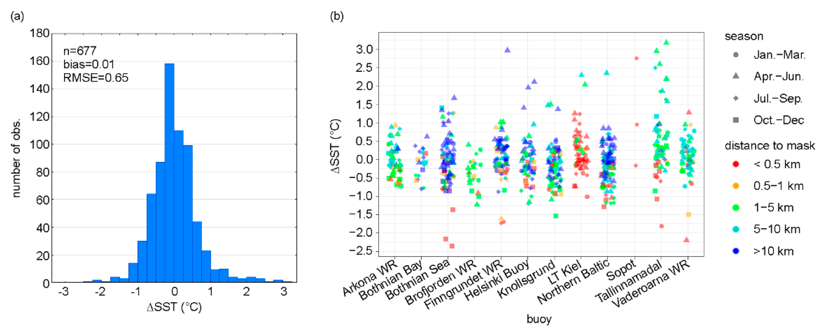
As shown in Figure 8, outlying residuals—both positive and negative—may be found over the entire range of temperature considered. Differences between SSTs estimated using the most accurate input data (Collection 2) and NLSST Equation (v1) were within the range of −2.36 °C to 3.18 °C. Outliers increased the RMSE to 0.65 °C (Figure 9a) and bias to 0.01 °C. The highest negative residuals (ΔSST less than −1.25 °C) occurred at a distance of less than 0.5 km to a maximum of 1 km from the mask (Figure 9b). Detailed analysis of the spatial distribution of SSTs and images from the OLI instrument suggested that it was the result of insufficient masking of the cloud effect. Overestimation of the reference temperature by more than 1 °C was most often recorded in May and June for buoys located in the Gulf of Finland and the Bothnian Sea (Figure 9b) and fixed platforms—Tallinamandal, Sopot and LT Kiel. In the case of offshore platforms, the higher temperature of infrastructure in the proximity (a lighthouse or pier) was the most probable reason for positive outliers. High SST residuals, both positive and negative, were also observed when in situ measurements were taken near thermal fronts resulting from the proximity of different water masses. The difference may therefore be biased by an inaccurate location of the measurement (the fixed position of the buoy was taken into account).

4. Summary and Conclusions

In order to use L1 satellite data for SST mapping, at least two issues need to be addressed: filtering erroneous data due to the influence of clouds, ice or land and calculating surface temperature from brightness temperature affected by absorption in the atmosphere.
With respect to the first issue, products of two different approaches were used: traditional, based on decision trees (CFMask algorithm) and a modern approach based on a neural network (the IdePix algorithm). It was noticed that the IdePix flag marking pixels as “ambiguous” may lead to overmasking. Nevertheless, this flag has proven to be useful for improving the CFMask product after correction based on the analysis of adjacent pixels. An effective mask should eliminate as many erroneous values as possible (high negative residuals as an indicator), leaving as many appropriate pixels as possible. Maintaining a balance between these two results in greater uncertainty of the SST estimation near the mask if more advanced cloud screening techniques are not applied. The advantage of both algorithms is the availability of their products or a ready-to-use tool. However, cloud detection techniques are still developing, and many other advanced algorithms could be applied [14,48], both those developed for Landsat and those used for satellite missions dedicated to measuring SST. In particular, using radiative transfer simulations under clear sky conditions to only the IR channels, could eliminate the issue observed with IdePix.
As mentioned in the literature review, the researchers in [36] showed that SSTs may be estimated from Landsat 8/TIRS data with good accuracy using the NLSST formula (Equations (1) and (2)). The authors derived best-fit coefficients empirically on the basis of in situ measurements. Therefore, one of the questions in this study was whether coefficients derived for the region with a more humid atmosphere might be applicable to the Baltic Sea. The comparison estimated SSTs and the data from buoys showed relatively good accuracy of the SST estimation, which slightly decreases as the temperature drops below 10 °C. This trend is related to the change in air humidity rather than water temperature itself. There is a strong indication that the relationship between split-window difference and SST changes if the difference is lower than 1.0 °C [41]. Cases with a difference in TIRS bands less than 1 °C accounted for 49% of analysed matchups and more than 76% of them were characterized by the in situ temperature below 10 °C. NLSST formula with coefficients derived for the Baltic Sea reduced this trend and bias.
The improved radiometric calibration applied to the USGS Collection 2 dataset resulted in a reduction in both the brightness temperature at band 10 (~11 µm) and the split window difference. Therefore, the NLSST coefficients should be determined separately for these data; otherwise, the SSTs would be underestimated, with the error increasing with surface temperature. Nevertheless, contrary to expectations, this study did not find a significant improvement in RMSE using recalibrated data. The NLSST algorithm with best-fit coefficients derived for the Baltic Sea estimated SST using the most accurate input data (Collection 2) with an RMSE 0.5 °C. These results match those observed in earlier studies [28,33,36] or reported for standard SST products of lower resolution, validated against in situ bulk temperatures measured in the Baltic Sea [1,4,6,13,16,19,20]. Taking into account changes in the path length through the atmosphere despite the relatively low satellite viewing angle turned out to have an impact on the results. The use of a simplified version of the algorithm more often resulted in underestimating the SSTs. To improve the performance of the NLSST formula, sets of temporal and spatial dependent coefficients should be derived in order to reflect variations in the atmospheric regimes [40]. The selected set of matchups was too small to analyse this approach. The development of the Baltic Sea Oceanographic Operational System, which currently provides a significant number of real-time observations (e.g., from tidal stations, FerryBox lines, mooring buoys, fixed stations, Argo profilers and research vessels) [30] should allow for such analysis in the near future. Further improvement may be achieved using climatological SST data records as an SST first guess, instead of MCSST. Jang and Park [36] found that the OSTIA data provided by the Met Office allow the RMSE to be slightly reduced. A 30 year climate data record for the North Sea and Baltic Sea region of SST has been produced by [1].
For standard SST products derived from nighttime satellite overpasses, insufficient cloud masking is the source of the highest uncertainties. The Landsat mission provides only daytime observations on a regular basis. Therefore, another significant source of uncertainty is daily heating, which is manifested more strongly in the subsurface layer than at the depth at which the temperature is measured in situ (bulk temperature). The IR radiances measured by the satellite instrument only respond to the temperature which represents a 10-µm surface layer. Even if the NLSST coefficients are calibrated against in situ data, the relationship reflects only the average difference between temperatures of different layers while the daily heating varies over time and space depending on wind and irradiance conditions [49]. In the Baltic Sea, diurnal warming of the sea surface (day/ night temperature difference) for the most part does not exceed 3 °C, though events with daily anomalies over 5 K can be observed. Satellite/in situ observations from moored buoys have much smaller average differences ranging from −0.3 °C to 0.1 °C [15]. Although high positive residuals for Landsat SST estimation occurred in late spring and summer, they cannot be related to these effects. In most cases they appeared to be errors connected with the influence of different objects or platforms within a Landsat pixel. However, the range of differences between bulk and skin temperature reported by [15] indicates that the effects of diurnal warming may have a large impact on the RMSE obtained for the NLSST algorithm in the Baltic Sea. Another source of uncertainty for high-spatial-resolution data may be horizontal temperature gradients if the in situ measurement location is not accurately determined.
The NLSST algorithm applied to the newly reprocessed Landsat 8 data gives a realistic estimate of values and maps comparable to the products of long-term earth observation missions, e.g., AQUA MODIS (Figure 10). As this is a simple statistical approach, its accuracy cannot be as high as with the more physical methods that are now becoming standard in satellite remote sensing of sea surface temperature, e.g., optimal estimation. An overview of methods with claims of improved accuracy is given by [14]. However, in many issues where the accuracy of estimating the SST is less important than possibility of identifying phenomena and their spatial variability, the simplicity of the NLSST algorithm can be a great advantage. Landsat data can be accessed in different ways, both through an interactive service (e.g., Earth Explorer) or with a Machine-to-Machine API. The USGS also provide tools to create the angle bands needed for the full NLSST algorithm and Quality Assessment TOOLS. There are also others, e.g., SNAP or QGIS plugins, Python and R packages that can be used to select, download and process Landsat data. Some of them may not yet support the new structure of metadata stored in Collection 2. However, it has been shown that the data from Collection 1, which will be available by December 2022, and the NLSST coefficients determined for the Baltic Sea, allow the estimation of SSTs with similar accuracy.

Funding

This research was supported by the University of Gdansk, Division of Physical Oceanog.

Data Availability Statement

Data available on request.

Acknowledgments

The study was made possible thanks to free access to data provided by the USGS (https://www.usgs.gov/ accessed on 1 March 2021), CMEMS (https://marine.copernicus.eu/ accessed on 1 March 2021) and free open source tools: SNAP (https://step.esa.int/ accessed on 1 March 2021) and R software (https://www.r-project.org/ accessed on 1 March 2021).

Conflicts of Interest

The author declares no conflict of interest.

References

  1. Høyer, J.L.; Karagali, I. Sea Surface Temperature Climate Data Record for the North Sea and Baltic Sea. J. Clim. 2016, 29, 2529–2541. [Google Scholar] [CrossRef]
  2. Leppäranta, M.; Myrberg, K. Physical Oceanography of the Baltic Sea; Series in Geophysical Sciences; Springer: Chichester, UK, 2009; ISBN 978-3-540-79702-9. [Google Scholar]
  3. Kniebusch, M.; Meier, H.E.M.; Neumann, T.; Börgel, F. Temperature Variability of the Baltic Sea since 1850 and Attribution to Atmospheric Forcing Variables. J. Geophys. Res. Ocean. 2019, 124, 4168–4187. [Google Scholar] [CrossRef]
  4. Stramska, M.; Białogrodzka, J. Spatial and Temporal Variability of Sea Surface Temperature in the Baltic Sea Based on 32-Years (1982–2013) of Satellite Data. Oceanologia 2015, 57, 223–235. [Google Scholar] [CrossRef] [Green Version]
  5. Gurova, E.; Chubarenko, B. Remote-Sensing Observations of Coastal Sub-Mesoscale Eddies in the South-Eastern Baltic. Oceanologia 2012, 54, 631–654. [Google Scholar] [CrossRef] [Green Version]
  6. Lehmann, A.; Myrberg, K.; Höflich, K. A Statistical Approach to Coastal Upwelling in the Baltic Sea Based on the Analysis of Satellite Data for 1990–2009. Oceanologia 2012, 54, 369–393. [Google Scholar] [CrossRef] [Green Version]
  7. O’Carroll, A.G.; Armstrong, E.M.; Beggs, H.M.; Bouali, M.; Casey, K.S.; Corlett, G.K.; Dash, P.; Donlon, C.J.; Gentemann, C.L.; Høyer, J.L.; et al. Observational Needs of Sea Surface Temperature. Front. Mar. Sci. 2019, 6, 420. [Google Scholar] [CrossRef]
  8. Kahru, M.; Elmgren, R.; Kaiser, J.; Wasmund, N.; Savchuk, O. Cyanobacterial Blooms in the Baltic Sea: Correlations with Environmental Factors. Harmful Algae 2020, 92, 101739. [Google Scholar] [CrossRef]
  9. Kahru, M.; Leppánen, J.-M.; Rud, O. Cyanobacterial Blooms Cause Heating of the Sea Surface. Mar. Ecol. Prog. Ser. 1993, 101, 1–7. [Google Scholar] [CrossRef]
  10. Morel, A.; Antoine, D. Heating Rate within the Upper Ocean in Relation to Its Bio-Optical State. J. Phys. Geogr. 1994, 24, 1652–1655. [Google Scholar] [CrossRef] [Green Version]
  11. Matciak, M.; Wojtasiewicz, B. Field Investigation on Seawater Temperature Variability in Relation to Horizontal Optical Gradient. J. Mar. Res. 2007, 65, 737–757. [Google Scholar] [CrossRef]
  12. Konik, M. Remote Sensing of Cyanobacteria Blooms and Their Influence on the Remotely Sensed Physical Properties of the Water in the Baltic Sea. Ph.D. Thesis, Institute of Oceanology of the Polish Academy of Sciences, Sopot, Poland, 2021. [Google Scholar]
  13. Konik, M.; Kowalewski, M.; Bradtke, K.; Darecki, M. The Operational Method of Filling Information Gaps in Satellite Imagery Using Numerical Models. Int. J. Appl. Earth Obs. Geoinf. 2019, 75, 68–82. [Google Scholar] [CrossRef]
  14. Minnett, P.J.; Alvera-Azcárate, A.; Chin, T.M.; Corlett, G.K.; Gentemann, C.L.; Karagali, I.; Li, X.; Marsouin, A.; Marullo, S.; Maturi, E.; et al. Half a Century of Satellite Remote Sensing of Sea-Surface Temperature. Remote Sens. Environ. 2019, 233, 111366. [Google Scholar] [CrossRef]
  15. Karagali, I.; Høyer, J.; Hasager, C. SST Diurnal Variability in the North Sea and the Baltic Sea. Remote Sens. Environ. 2012, 121, 159–170. [Google Scholar] [CrossRef]
  16. Kozlov, I.; Dailidienė, I.; Korosov, A.; Klemas, V.; Mingėlaitė, T.T. MODIS-Based Sea Surface Temperature of the Baltic Sea Curonian Lagoon. J. Mar. Syst. 2014, 129, 157–165. [Google Scholar] [CrossRef]
  17. Losa, S.N.; Danilov, S.; Schröter, J.; Nerger, L.; Maβmann, S.; Jenssen, F. Assimilating NOAA SST Data into the BSH Operational Circulation Model for the North and Baltic Seas: Inference about the Data. J. Mar. Syst. 2012, 105–108, 152–162. [Google Scholar] [CrossRef] [Green Version]
  18. Liu, Y.; Fu, W. Assimilating High-Resolution Sea Surface Temperature Data Improves the Ocean Forecast Potential in the Baltic Sea. Ocean Sci. 2018, 14, 525–541. [Google Scholar] [CrossRef] [Green Version]
  19. Woźniak, B.; Krężel, A.; Darecki, M.; Woźniak, S.B.; Majchrowski, R.; Ostrowska, M.; Kozłowski, Ł.; Ficek, D.; Olszewski, J.; Dera, J. Algorithm for the Remote Sensing of the Baltic Ekosystem (DESAMBEM), Part 1: Mathematical Apparatus. Oceanologia 2008, 50, 451–508. [Google Scholar]
  20. Høyer, J.L.; She, J. Optimal Interpolation of Sea Surface Temperature for the North Sea and Baltic Sea. J. Mar. Syst. 2007, 65, 176–189. [Google Scholar] [CrossRef]
  21. Li, J.; Chen, B. Global Revisit Interval Analysis of Landsat-8-9 and Sentinel-2A-2B Data for Terrestrial Monitoring. Sensors 2020, 20, 6631. [Google Scholar] [CrossRef]
  22. Landsat 8 (L8) Data Users Handbook; LSDS-1574 v.5.0; Department of the Interior U.S. Geological Survey, EROS: Sioux Falls, SD, USA, 2019. Available online: https://www.usgs.gov/media/files/landsat-8-data-users-handbook (accessed on 1 September 2021).
  23. Kuroda, H.; Toya, Y. High-Resolution Sea Surface Temperatures Derived from Landsat 8: A Study of Submesoscale Frontal Structures on the Pacific Shelf off the Hokkaido Coast, Japan. Remote Sens. 2020, 12, 3326. [Google Scholar] [CrossRef]
  24. Brando, V.E.; Braga, F.; Zaggia, L.; Giardino, C.; Bresciani, M.; Matta, E.; Bellafiore, D.; Ferrarin, C.; Maicu, F.; Benetazzo, A.; et al. High-Resolution Satellite Turbidity and Sea Surface Temperature Observations of River Plume Interactions during a Significant Flood Event. Ocean Sci. 2015, 11, 909–920. [Google Scholar] [CrossRef] [Green Version]
  25. Xing, Q.; Braga, F.; Tosi, L.; Lou, M.; Zaggia, L.; Teatini, P.; Gao, X.; Yu, L.; Wen, X.; Shi, P. Detection of Low Salinity Groundwater Seeping into the Eastern Laizhou Bay (China) with the Aid of Landsat Thermal Data. J. Coast. Res. 2016, 74, 149–156. [Google Scholar] [CrossRef]
  26. Trinh, R.C.; Fichot, C.G.; Gierach, M.M.; Holt, B.; Malakar, N.K.; Hulley, G.; Smith, J. Application of Landsat 8 for Monitoring Impacts of Wastewater Discharge on Coastal Water Quality. Front. Mar. Sci. 2017, 4, 329. [Google Scholar] [CrossRef] [Green Version]
  27. Savari, A.; Dehmordi, L.M.; Dostshenas, A.; Asgari, H.M.; Abasi, A. Assessment of Chlorophyll-a, SST and Diffuse Attenuation Coefficient (Kd490) in Northwest of Persian Gulf Using Landsat 8 Satellite Data. Int. J. Sci. 2016, 5, 10–26. [Google Scholar] [CrossRef] [Green Version]
  28. Snyder, J.; Boss, E.; Weatherbee, R.; Thomas, A.C.; Brady, D.; Newell, C. Oyster Aquaculture Site Selection Using Landsat 8-Derived Sea Surface Temperature, Turbidity, and Chlorophyll a. Front. Mar. Sci 2017, 4, 190. [Google Scholar] [CrossRef] [Green Version]
  29. Cahyono, A.B.; Saptarini, D.; Pribadi, C.B.; Armono, H.D. Estimation of Sea Surface Temperature (SST) Using Split Window Methods for Monitoring Industrial Activity in Coastal Area. Appl. Mech. Mater. 2017, 862, 90–95. [Google Scholar] [CrossRef]
  30. She, J.; Meier, H.E.M.; Darecki, M.; Gorringe, P.; Huess, V.; Kouts, T.; Reissmann, J.H.; Tuomi, L. Baltic Sea Operational Oceanography—A Stimulant for Regional Earth System Research. Front. Earth Sci. 2020, 8, 7. [Google Scholar] [CrossRef]
  31. Syariz, M.A.; Jaelani, L.M.; Subehi, L.; Pamungkas, A.; Koenhardono, E.S.; Sulisetyono, A. Retrieval of Sea Surface Temperature over Poteran Island Water of Indonesia with Landsat 8 TIRS Image: A Preliminary Algorithm; The International Archives of the Photogrammetry, Remote Sensing and Spatial Information Sciences: Kuala Lumpur, Malaysia, 2015; Volume XL-2/W4, pp. 87–90. [Google Scholar]
  32. Susilo, E.; Hanintyo, R.; Wijaya, A. Retrieving Coastal Sea Surface Temperature from Landsat-8 TIRS for Wangi-Wangi Island, Wakatobi, Southeast Sulawesi, Indonesia. Int. J. Remote Sens. Earth Sci. 2019, 16, 13–22. [Google Scholar] [CrossRef]
  33. Vanhellemont, Q. Automated Water Surface Temperature Retrieval from Landsat 8/TIRS. Remote Sens. Environ. 2020, 237, 111518. [Google Scholar] [CrossRef]
  34. Barsi, J.A.; Schott, J.R.; Hook, S.J.; Raqueno, N.G.; Markham, B.L.; Radocinski, R.G. Landsat-8 Thermal Infrared Sensor (TIRS) Vicarious Radiometric Calibration. Remote Sens. 2014, 6, 11607–11626. [Google Scholar] [CrossRef] [Green Version]
  35. Gerace, A.; Montanaro, M. Derivation and Validation of the Stray Light Correction Algorithm for the Thermal Infrared Sensor Onboard Landsat 8. Remote Sens. Environ. 2017, 191, 246–257. [Google Scholar] [CrossRef]
  36. Jang, J.-C.; Park, K.-A. High-Resolution Sea Surface Temperature Retrieval from Landsat 8 OLI/TIRS Data at Coastal Regions. Remote Sens. 2019, 11, 2687. [Google Scholar] [CrossRef] [Green Version]
  37. Bayat, F.; Hasanlou, M. Feasibility Study of Landsat-8 Imagery for Retrieving Sea Surface Temperature (Case Study Persian Gulf); The International Archives of the Photogrammetry, Remote Sensing and Spatial Information Sciences: Prague, Czech Republic, 2016; Volume XLI-B8, pp. 1107–1110. [Google Scholar]
  38. Walton, C.C.; Pichel, W.G.; Sapper, F.; May, D.A. The Development and Operational Application of Nonlinear Algorithms for the Measurement of Sea Surface Temperatures with the NOAA Polar-Orbiting Environmental Satellites. J. Geophys. Res. 1998, 103, 27999–28012. [Google Scholar] [CrossRef]
  39. Appendix, G. (Ed.) NOAA KLM User’s Guide with NOAA-N, N Prime, and MetOp Supplements; U.S. Department of Commerce, National Oceanic and Atmospheric Administration, National Environmental Satellite, Data, and Information Service, National Climatic Data Center, Climate Services Division, Satellite Services Branch: Asheville, NC, USA, 2014.
  40. Kilpatrick, K.; Podestá, G.; Evans, R. Overview of the NOAA/NASA Pathfinder Version 4.2 Algorithm for Sea Surface Temperature and Associated Matchup Database. J. Geophys. Res. 2001, 106, 9179–9197. [Google Scholar] [CrossRef]
  41. Emery, W.J.; Yu, Y.; Wick, G.A.; Schlüssel, P.; Reynolds, R.W. Correcting Infrared Satellite Estimates of Sea Surface Temperature for Atmospheric Water Vapor Attenuation. J. Geophys. Res. 1994, 99, 5219–5236. [Google Scholar] [CrossRef]
  42. U.S. Geological Survey Landsat Collection 2 (Version 1.1, 15 January, 2021); U.S. Geological Survey Fact Sheet 2021-3002; U.S. Geological Survey: Washington, DC, USA, 2021; 4p. [CrossRef]
  43. Copernicus Marine In Situ TAC. Copernicus Marine In Situ TAC Quality Information Document for Near Real Time In Situ Products (QUID and SQO). V2.1; Copernicus Marine In Situ TAC: 2021. Available online: https://archimer.ifremer.fr/doc/00646/75807/ (accessed on 1 March 2021). [CrossRef]
  44. Liu, H.; Shah, S.; Jiang, W. On-Line Outlier Detection and Data Cleaning. Comput. Chem. Eng. 2004, 28, 1635–1647. [Google Scholar] [CrossRef]
  45. Landsat 8 Operational Land Imager (OLI)—Thermal Infrared Sensor (TIRS) Solar and View Angle Generation Algorithm de-Scription Document (Add). LSDS-1928 v.2.0. 2018. Available online: https://www.usgs.gov/media/files/lsds-1928-landsat-8-olitirs-solar-view-angle-generation-add (accessed on 1 September 2021).
  46. Zhu, Z.; Wang, S.; Woodcock, C.E. Improvement and Expansion of TheFmask Algorithm: Cloud, Cloud Shadow, and Snow Detection for Landsats 4–7,8, and Sentinel 2 Images. Remote Sens. Environ. 2015, 159, 269–277. [Google Scholar] [CrossRef]
  47. Landsat 8–9 Operational Land Imager (OLI)—Thermal Infrared Sensor (TIRS) Collection 2 Level 1 (L1) Data Format Control Book (DFCB). LSDS-1822 Version 6.0. 2020. Available online: https://www.usgs.gov/media/files/landsat-8-9-olitirs-collection-2-level-1-data-format-control-book (accessed on 1 September 2021).
  48. Mahajan, S.; Fataniya, B. Cloud Detection Methodologies: Variants and Development—A Review. Complex Intell. Syst. 2020, 6, 251–261. [Google Scholar] [CrossRef] [Green Version]
  49. Minnett, P.J. Radiometric Measurements of the Sea-Surface Skin Temperature: The Competing Roles of the Diurnal Thermocline and the Cool Skin. Int. J. Remote Sens. 2003, 24, 5033–5047. [Google Scholar] [CrossRef]
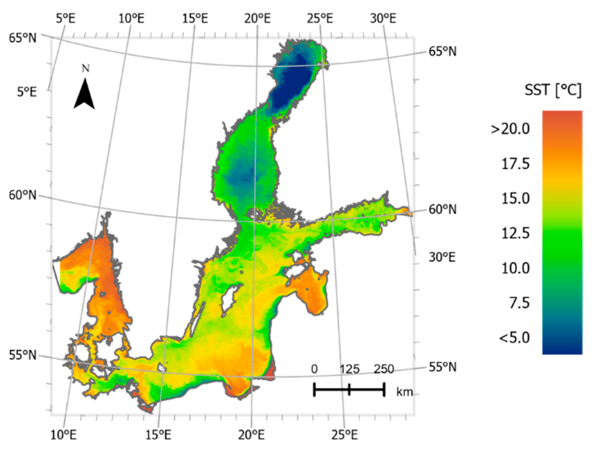
Figure 1. Spatial distribution of the sea surface temperature influenced by coastal processes (data provided by System SatBaltyk www.satbaltyk.iopan.gda.pl; merged SST product [13]; 31 May 2018 06:00 UTC).
Remotesensing 13 04619 g001
Figure 2. Locations of the in situ reference buoys/stations and footprints of Landsat 8 processed granules.
Remotesensing 13 04619 g002
Figure 3. Example of in situ temperature data before (red) and after Hampel filtration (green). Data selected for comparison with satellite data are marked with dots.
Remotesensing 13 04619 g003
Figure 4. Satellite-derived SST (estimated using NLSST formula with the coefficients ai and bi given by [36] applied to Collection 1 TIRS data) versus in situ reference temperature for all matchups (a) and statistics of SST residuals for pixels classified initially as clear on the base of quality assessment flags (QA mask) (b).
Remotesensing 13 04619 g004
Figure 5. Distribution of SST residuals with different masks applied to exclude erroneous pixels (red bars): QA mask extended with the IdePix flags (a), QA mask extended with the IdePix flags and buffer (b), QA mask extended with corrected IdePix flags and buffer (c). Distribution of residuals with initial QA mask is shown for comparison (blue bars).
Remotesensing 13 04619 g005
Figure 6. Examples of two types of problems when masking with a combination of QA mask and IdePix flags: omission error—the boundary pixels issue (13 January 2015) and commission error—the cloud ambiguous flag issue (16 February 2015). Maps present SST values after the QA, the IdePix and buffer combined mask application (a,b), SST values calculated for all pixels (c,d) ang RGB composites (e,f).
Remotesensing 13 04619 g006
Figure 7. Landsat 8 image example—RGB composite (a) and derived SST map using different masks to exclude erroneous pixels: no mask (b), QA mask (c), a combination of QA mask and the IdePix flags with additional corrections (d) and an SST map derived from MODIS data recorded on the same day (e) for comparison (MODIS data provided by System SatBaltyk).
Remotesensing 13 04619 g007
Figure 8. Satellite-derived SST versus in situ reference temperatures for different data sources: Collection 1 (ac) and Collection 2 (df) and different sets of coefficients: derived by [36]—listed in Section 2.3 (a,d) and derived for the Baltic Sea—listed in Table 2 (b,c,e,f) for the full (v1) and simplified (v2) version of the NLSST algorithm. Outliers are presented but not included in the analysis.
Remotesensing 13 04619 g008
Figure 9. Distribution of SST residuals (ΔSST) calculated using the NLSST v2 algorithm and brightness temperatures from USGS Collection 2 L1 data (a) and their spatial and temporal variability (b).
Remotesensing 13 04619 g009
Figure 10. SST maps derived from Landsat 8 TIRS data from 19 September 2015 (a,b) and 17 May 2013 (c,d) using NLSST algorithm (v1, Collection 2) (left panel) and L2 AQUA/MODIS product (right panel). MODIS data provided by System SatBaltyk.
Remotesensing 13 04619 g010
Table 1. Basic characteristics of in situ data sources and the number of matchups before (all) and after (clear) contaminated pixel masking.
NameTypePositionSampling
Interval
(h)
Depth (m)
Measurement/Bottom *
Number of Matchups
All/Clear
Arkona WRwave buoy13.87°E 54.88°N10.5/4583/55
Bothnian Baywave buoy23.24°E 64.68°N0.50.5/7529/20
Bothnian Seawave buoy20.23°E 61.80°N0.50.5/110161/91
Brofjorden WRwave buoy11.22°E 58.25°N0.50.5/5540/22
Fingrundet WRwave buoy18.61°E 60.9°N0.50.5/68131/76
Helsinki Buoywave buoy25.24°E 59.97°N0.50.5/5097/57
Knollsgrundwave buoy17.62°E 57.52°N10.5/95126/80
LT Kielfixed platform10.27°E 54.50°N10.5/1399/54
Northern Balticwave buoy21.00°E 59.25°N0.50.5/95173/100
Sopotfixed platform18.58°E 54.45°N1subsurface/842/3
Tallinnamadalfixed platform24.73°E 59.71°N1subsurface/10140/59
Vaderoarnawave buoy10.93°E 58.50°N0.50.5/7092/63
* data source: Baltic Sea Hydrographic Commission, 2013, Baltic Sea Bathymetry Database version 0.9.3. Downloaded from http://data.bshc.pro/, accessed on 20 October 2021.
Table 2. Coefficients of the NLSST algorithms (full and simplified version of Equations (1) and (2)) estimated with nonlinear regression and two different sources of TIRS data as an input, and their statistical characteristics.
CoefficientInput Data: Collection 1Input Data: Collection 2
EstimateStd. Errorp-ValueREstimateStd. Errorp-ValueR
NLSST v1 (full):
SST = a1T11 + a2(T11 − T12)MCSST + a3(T11 − T12)(secθsat − 1) + a4,
MCSST = b1T11 + b2(T11 − T12) + b3(T11 − T12)(secθsat − 1) + b4
a10.9220.0090.0000.9960.9390.0060.0000.997
a20.0860.0040.0000.0920.0050.000
a318.9157.4740.00936.55410.4060.000
a4−250.8292.3910.000−254.7531.7590.000
b10.9980.0060.0000.9960.9900.0050.0000.996
b21.3480.0640.0001.2910.0710.000
b312.3997.4470.09718.52511.5410.109
b4−272.4681.5780.000−268.9611.4110.000
NLSST v2 (simplified):
SST = a1T11 + a2(T11 − T12)MCSST + a3,
MCSST = b1T11 + b2(T11 − T12) + b3
a10.9200.0090.0000.9960.9370.0060.0000.997
a20.0900.0040.0000.1010.0040.000
a3−250.3692.3890.000−254.2201.7790.000
b10.9990.0060.0000.9960.9900.0050.0000.996
b21.3870.0590.0001.3550.0590.000
b3−272.6471.5770.000−269.1171.4100.000
R—nonlinear correlation coefficient.
Publisher’s Note: MDPI stays neutral with regard to jurisdictional claims in published maps and institutional affiliations.