Spatio-Temporal Analysis of Ecological Vulnerability and Driving Factor Analysis in the Dongjiang River Basin, China, in the Recent 20 Years

Abstract

The global ecological environment faces many challenges. Landsat thematic mapper time-series, digital elevation models, meteorology, soil types, net primary production data, socio-economic data, and auxiliary data were collected in order to construct a comprehensive evaluation system for ecological vulnerability (EV) using multi-source remote sensing data. EV was divided into five vulnerability levels: potential I, slight II, mild III, moderate IV, and severe V. Then, we analyzed and explored the spatio-temporal patterns and driving mechanisms of EV in the region over the past 20 years. Our research results showed that, from 2001 to 2019, the DRB was generally characterized as being in the severe vulnerability class, with higher upstream and downstream EV classes and a certain amount of reduction in the midstream EV classes. Moreover, EV in the DRB continues to decrease. The spatio-temporal EV patterns in the DRB were significantly influenced by the relative humidity, average annual temperature, and vegetation cover over the past 20 years. Our work can provide a basis for decision-making and technical support for ecosystem protection, ecological restoration, and ecological management in the DRB.

1. Introduction

Since the middle of the 20th century, the intensification of human activities has led to frequent climate-change-related disasters [1,2,3,4] and the intensification of ecological and environmental crises [5]. These scenarios pose serious challenges to the ecosystems on which humans depend for their survival. Among them, the issue of ecological vulnerability (EV) is particularly prominent. EV was first introduced into ecological theory by Clements as an “ecological staggering zone” [6,7] and was further discussed at the seventh SCOPE (Scientific Committee of Environmental Problems) Conference in 1989 [6,8,9]. The ability of a system to resist external environmental change and to be disturbed and recover itself is defined as EV [10,11,12,13]. EV is determined by a combination of internal and external vulnerability [14,15]. Internal vulnerability usually stems from the structure of the ecosystem itself and is mainly influenced by natural conditions such as topography and climate. External vulnerability is influenced by human activities [16]. Exploring regional EV is important for ecological change and socio-economic development.

Scholars around the world have conducted relevant studies on the spatio–temporal evolution patterns of EV and its driving mechanisms [2,13,17,18,19,20,21,22,23]. Most of these EV studies are focused on China [21] and can be based on individual cities or regions [24], e.g., on the northwestern part of the Songnun Plain [17], the Tibetan Plateau [18], the Loess Plateau [19], the southwestern karst mountains [10], agricultural and pastoral areas [22], coal mining areas [2], the southern Shaanxi region [25], islands [26], coastal wetlands [27]; there are also studies that focus on the Bangladesh–China–India–Myanmar economic corridor [21]. Recently, the ecology of red loam hilly areas in southern China has become a focus of attention for many scholars [28].

Dongjiang is the third largest water system in the Pearl River basin and belongs to the South China basin, which is characterized as having a typical tropical–subtropical climate. The Dongjiang River Basin (DRB) is located in the red-loamy hilly region of southern China, which, as a pioneering region for reform and opening up, has seen a rapid economic development over the past 40 years. China’s 13th Five-Year Plan supports the construction of an open and innovative transformation of the Pearl River Delta region, namely the Guangdong–Hong Kong–Macao Greater Bay Area. Meanwhile, the DRB is an important drinking water source for the Pearl River Delta and Hong Kong and an essential focus of the sustainable development strategy in the Pearl River Delta region. The socio-economic development of the basin and changes in the natural environment affect the quality of the ecological environment and the sustainable use of resources in the basin [29]. With accelerated urbanization, dramatic climate change, and increased disturbance from human activities, the quality of the ecological environment in the DRB faces unprecedented threats, and thus the DRB has become an ideal area for analyzing EV. Hu [24] used the AHP method to evaluate the EV of Weifang city, China; however, the study used limited the quantitative data and was heavily dependent on qualitative inputs. These factors led to unconvincing results, especially when there were many factors, and it was difficult to precisely determine the weights. Wu [30] used the fuzzy hierarchical analysis method to evaluate the EV of the Yellow River Delta; however, there were drawbacks related to the subjective factor weights and large computational effort. Principal component analysis (PCA) is one of the most commonly used methods for model evaluation, as it can reduce data complexity, identify the most important multiple features, and save significant computational resources, and is easily implemented on a computer. In this paper, PCA was used to model and analyze the time-series EV in the DRB.

Factors commonly used in EV assessment can be divided into two categories: those reflecting human activities, such as population density, GDP per capita, etc.; and ecological and natural conditions, such as slope, temperature, precipitation, vegetative cover, etc. As a result of the complexity of human–nature interactions, there is currently no uniform standard for the selection of factors for EV assessment models [31]. Moreover, there is the problem of regional adaptability in EV assessment models [22]. The ecological environment in the red soil hilly areas of southern China is fragile [32]; furthermore, there is a lack of an EV zoning system. In addition, many of the current studies on EV are analyzed at a regional scale and are less specific to county EV evaluations. Therefore, there is a need to develop a reliable methodology to assess EV in the DRB.

Our work established a dynamic evaluation scheme for monitoring the spatio-temporal EV changes in the DRB and calculated the dynamic EV weights in 2001–2019 using PCA. Finally, we analyzed the spatio-temporal evolution of EV in the DRB and its driving mechanisms over the past 20 years. The research results and methods provide a theoretical basis and technical support for the protection and restoration of the environment within the DRB. The flowchart for this work is shown in Figure 1.

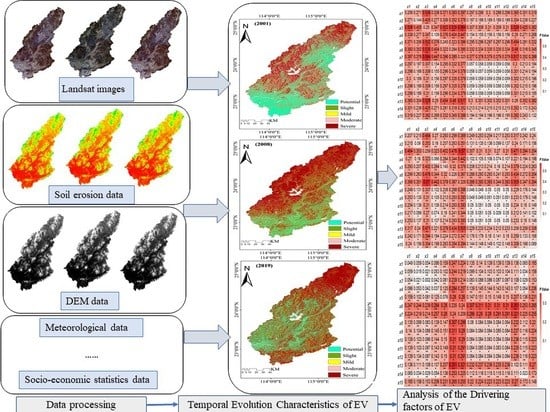
2. Materials and Methods

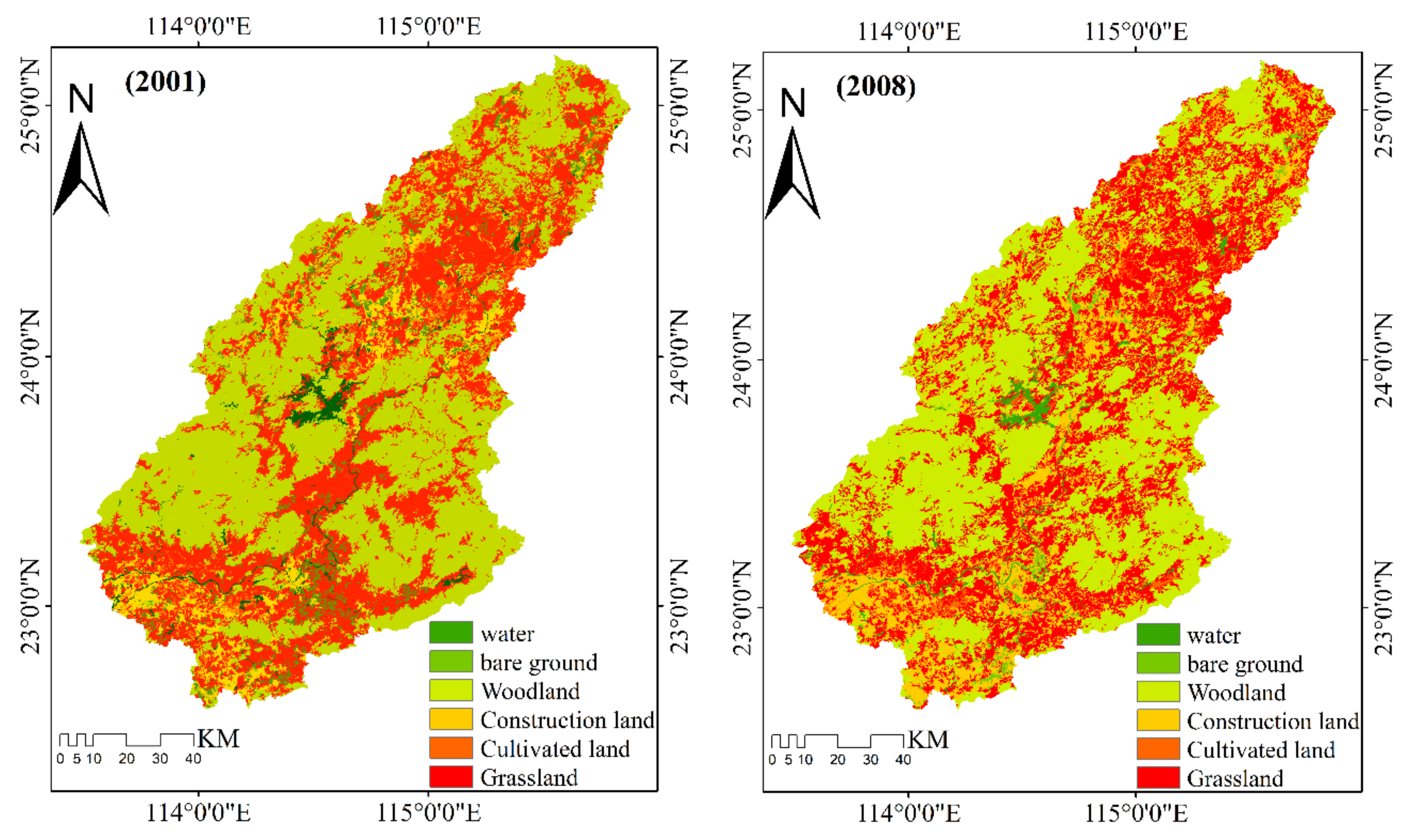
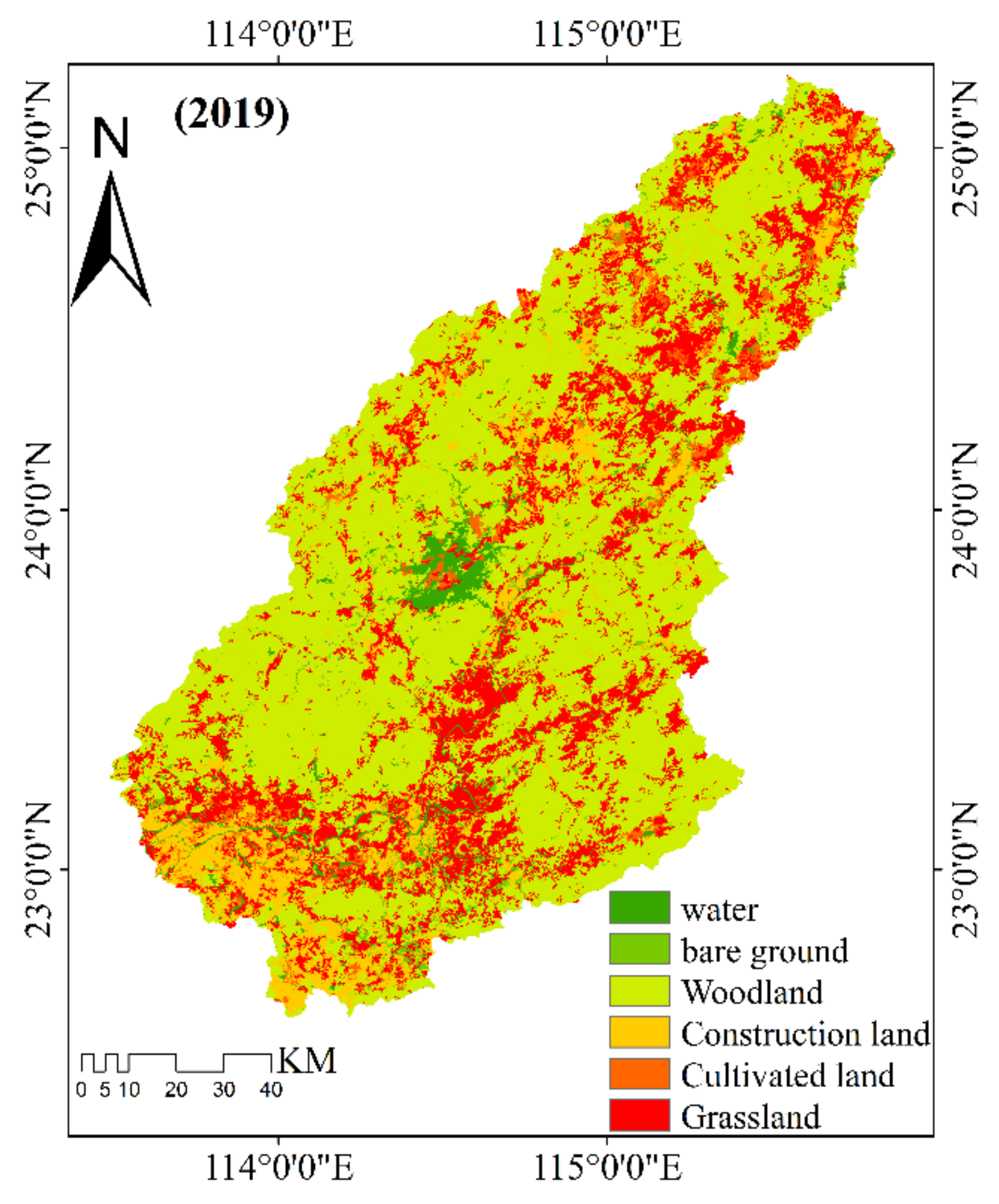
2.1. Study Area

The DRB (Figure 2) is connected to Meishan in eastern Guangdong; to its west, it is bordered by Shaoguan and Qingyuan in northern Guangdong; the South China Sea and Hong Kong lie to the south, and the Dongjiang source area of southern Ganzhou lies to the north. The geographical location of the DRB is 113°52′–115°52′ E and 22°38′–25°14′ N, with hilly mountains in the center and north. The DRB is a valuable water resource for social development within the basin, providing water to Hong Kong for production, living, and ecology, and to more than 40 million people who live in the urban clusters along the basin. The middle and lower reaches of the DRB are economically developed, and the total GDP of the regions in Guangdong, China, that are supported by Dongjiang water was RMB 4.17 trillion in 2019, accounting for approximately 39% of the total GDP of Guangdong Province.

2.2. Evaluation Factors and Data Sources

We studied the “China Guangdong Environmental Protection Department on the Comprehensive Water Environment Improvement Programme of the Dongjiang River Basin (2015–2020)”, combined with related studies [33,34,35], and considered the availability of relevant assessment factors. We selected factors from topography, climate, landscape, vegetation, and socio-economic aspects to construct an EV evaluation system. The data sources are shown in

Table 1. Data sources and characteristics.

Name of Data	Data Production Unit	Data Source Website	Resolution	Processing Method
Landsat remote sensing satellite data	USGS	https://earthexplorer.usgs.gov/	30 m	Spatial analysis
GDEMV2 Elevation Data	Geospatial Data Cloud	http://www.gscloud.cn/	30 m	Spatial analysis
GDP per capita	Statistical Yearbook of Jiangxi and Guangdong Province, China	_	_	Statistical analysis
1:4 million Chinese soil type data	National Earth System Science Data Sharing Platform	http://www.geodata.cn/	_	Spatial analysis
Population density	WorldPOP dataset	https://www.worldpop.org/	100 m	Spatial analysis
Meteorological data	China Weather Data website	http://data.cma.cn/	_	Spatial analysis

Note: We last accessed the link above on 16 November 2020.

. There were some differences as regards the data sources and spatial accuracies of the factors. In the Arc GIS10.1 software platform, the WGS 1984 coordinate system and Mercator projection were uniformly used to ensure acceptable spatial coincidences for the factors. Moreover, all of these were unified to a raster image element size of 30 × 30 m using the ArcGIS10.2 platform to accommodate subsequent spatial calculations. The data sources are shown in Table 1.

Topographic factors included elevation, slope, slope orientation, soil erosion, and other factors. The GDEMV2 elevation data, which have a 30 m spatial resolution covering 29 scenes in Jiangxi and 31 scenes in Guangdong, were mainly obtained from the Geospatial Data Cloud website (http://www.gscloud.cn/). Data such as elevation, slope, and slope direction were calculated from the DEM data [29]. Soil erosion is one of the major factors related to soil degradation worldwide [36,37,38]. The widely used soil loss equation model [39] was used to calculate soil erosion in the DRB. These data were resampled to 30 m in ArcGIS.

Climate factors included average annual precipitation, average annual temperature, and relative humidity. These data were mainly obtained from the China Meteorological Data website (http://data.cma.cn/), which catalogues 17 meteorological stations. The inverse distance weighting method is a reliable method for spatial distribution that takes full account of the geographical links between factors. The above data were obtained by interpolation with the inverse distance weight method in ArcGIS 10.2.

Landscape factors included the mean patch area, boundary density, Shannon diversity index, Shannon evenness index, and Simpson diversity index, from Landsat remote sensing satellite data from the USGS website. Landsat-8 maintained a basic consistency with Landsat 1–7 in terms of spatial resolution and spectral characteristics. The satellite has a total of 11 bands, i.e., bands 1–7, and 9 bands have a spatial resolution of 30 m; band 8 is a panchromatic band with a 15 m resolution; and bands 10 and 11 have a spatial resolution of 100 m; the satellite can achieve global coverage once every 16 days [40]. For the 12 scenes, Landsat satellite image data containing few clouds were selected and are detailed in Appendix A 

Table A1. Landsat image identifier, acquisition time, and type characteristics.

Image Identifier	Acquisition Time	Sensor Type	Track Number (ROW/PATH)	Sun Elevation/(°)	Solar Azimuth/(°)
LT05_L1TP_121043_20011121_20161209_01_T1	21/11/2001	TM	43/121	39.428	149.338
LT05_L1TP_121044_20011121_20161209_01_T1	21/11/2001		44/122	40.544	148.454
LT05_L1TP_122043_20011230_20161209_01_T1	30/12/2001		43/121	34.59	147.199
LT05_L1TP_122044_20081201_20161028_01_T1	30/12/2001		44/122	35.663	146.415
LT05_L1TP_121043_20081210_20161028_01_T1	10/12/2008	TM	43/121	36.556	150.666
LT05_L1TP_121044_20081210_20161028_01_T1	10/12/2008		44/122	37.69	149.878
LT05_L1TP_122043_20081201_20161028_01_T1	1/12/2008		43/121	37.903	150.895
LT05_L1TP_122044_20081201_20161028_01_T1	1/12/2008		44/122	39.041	150.076
LC08_L1TP_121043_20191123_20191203_01_T1	23/11/2019	OLI	43/121	41.304	155.234
LC08_L1TP_121044_20191107_20191115_01_T1	7/11/2019		44/122	46.471	152.692
LC08_L1TP_122043_20191114_20191202_01_T1	14/11/2019		43/121	43.436	154.605
LC08_L1TP_122044_20191114_20191202_01_T1	14/11/2019		44/122	44.634	153.701

. The calculation of landscape pattern indices, such as mean patch area [41], boundary density [41], Shannon diversity index [42], Shannon evenness index [42], and Simpson diversity index [42], was performed in Fragstats 4.2 as described at https://www.umass.edu/landeco/research/fragstats/documents/fragstats.help.4.2.pdf.

Vegetation factors, which comprise vegetative cover, were derived from Landsat remote sensing satellite data, as described in the previous subsection. The vegetative cover data were calculated using the linear spectral mixture model (LSMM) from Landsat remote sensing satellite data [43].

Socio-economic statistics included population density and GDP per capita. Population density data were sourced from the WorldPOP dataset, and GDP per capita data were sourced from the ‘Statistical Yearbook of Jiangxi Province’ [44] and the ‘Statistical Yearbook of Guangdong Province’ [45]. Population density and GDP per capita were selected to calculate the impact of socio-economic activities on the EV of the watershed. The above data were obtained using the inverse distance weighting method in ArcGIS 10.2.

2.3. The Principal Component Analysis

The main objective of this study was to establish a comprehensive factor system based on PCA theory for assessing EV in DRB. PCA is a method for converting existing variables into a small number of summary factors that can best represent the most original information [46]. We first calculate the contribution rate, then look at the value of the main factor contribution rate to determine how many main factors there are, and the cumulative contribution rate of the main factors is considered to be satisfactory at 90% or more [47]. This assessment method includes a series of processing steps, e.g., the selection of relevant factors, standardization, the determination of the variance of common factors, the calculation of weights, and finally EV assessment.

2.3.1. The PCA Structure of EV Based on the PSR (Ecological Pressure Ecological Sensitivity, Ecological Resilience)

EV is the combined result of PSR [25,29,48,49]. Both natural and social factors can constrain the development of EV. Therefore, EV can also affect the economic development of a region, bringing about a series of developmental problems such as poor economic activity, slow development of modern industries, and low per capita education [13]. By reviewing the relevant information on EV in the DRB and assessing the relevant factor systems selected by researchers for the southern hilly mountains [50,51,52,53,54,55], it was found that a causal relationship between man and nature can be established with the PSR model. The general aim of this study was to establish a comprehensive PSR evaluation system based on PCA theory, and our analysis and evaluation system contains a target level, a criterion level, and a factor level. Both human activities and natural conditions affect EV, and so the evaluation factor system should include these two factors [56,57]. We developed a system analysis model consisting of three levels and 15 factors (

Table A2. Data sources and evaluation indicators.

Target Layer	Criterion Layer	Indicator Layer	Name of Data	Positive and Negative	Weight of 2001	Weight of 2008	Weight of 2019
Ecological Response	Terrain indicators	Elevation(X1)	GDEMV2 elevation data	Negative	0.03598	0.01263	0.00885
		Slope(X2)		Positive	0.0185	0.00718	0.00407
		Slope orientation(X3)		Positive	0.24991	0.24989	0.2499
		soil erosion(X4)	1:4 million Chinese soil type data Meteorological Data	Positive	0.00021	0.00017	0.00008
		Average annual precipitation(X5)		Negative	0.08956	0.09075	0.20449
		Average annual temperature(X6)		Negative	0.04795	0.05347	0.10973
		Relative Humidity(X7)		Positive	0.17487	0.20386	0.11149
Ecological State	Landscape indicators	Mean Patch area (Area_mn) (X8)	Landsat remote sensing satellite data	Negative	0.00059	0.00003	0.00012
		Boundary density (ed) (X9)		Positive	0.00107	0.00042	0.00071
		Shannon Diversity Index (SHDI) (X10)		Positive	0.00059	0.00039	0.00058
		Shannon’s evenness index (SHEI) (X11)		Negative	0.00001	0.00003	0.00012
		Simpson diversity index (SIDI) (X12)		Negative	0.00001	0.00003	0.00012
	Vegetation indicators	Vegetation cover(X13)		Negative	0.24466	0.24056	0.24606
Ecological Pressure	Social indicators	Population density(X14)	Population density	Positive	0.00015	0.00009	0.00011
		GDP per capita(X15)	GDP density	Positive	0.13595	0.1405	0.06357

in the Appendix A). We consulted relevant experts from the Guangdong Dongjiang River Basin Authority to understand the current situation in the basin.

Ecological response factors are the most direct characteristics expressed by the long-term interactions of various factors within an ecosystem [29]. In the vicinity of the DRB, the topography is fragmented, it has varying heights of terrain, there are hilly mountains in the center and north, and deltas, lowlands, and coastal plains in the south; the DRB has a subtropical monsoon climate, with an average annual temperature of 21 °C and an average annual precipitation of 1750 mm, which is uneven and mainly concentrated in April–September [34]. Ecological sensitivity factors can be divided into topographic and climatic factors: topographic factors are selected for elevation, slope, slope orientation, and soil erosion, which directly contribute to increased soil erosion problems [58]; climatic factors include mean annual precipitation, average annual temperature, and relative humidity. The DRB is cloudy and rainy. The average annual temperature and precipitation are key climatic factors affecting the amount of vegetative production. Moreover, relative humidity can reflect vegetation transpiration, so it is crucial for ecological protection [59].

Ecological state factors have a role in protecting ecosystems and can be divided into landscape factors and vegetation factors. The mean patch area (mean patch area, area_mn) can reflect landscape heterogeneity. It can, on the one hand, constrain the minimum patches of the image landscape and, on the other hand, reflect the degree of fragmentation of the landscape [41]. The boundary density (edge density, ED) is an important factor for analyzing patch shape, as it indicates the extent to which the landscape is fragmented, i.e., the higher the value, the more the boundary is fragmented, the more dispersed the layout, and the more compact the patches [41]. The Shannon diversity index (SHDI) reflects the landscape heterogeneity, primarily used to assess the contribution of rare patches to information, i.e., the richer the land use, the greater the fragmentation in the landscape, the higher the value, and the less damage to the landscape [42]. The Shannon evenness index (SHEI) indicates the maximum likelihood of a given landscape, i.e., the richer the landscape, the healthier and more stable its ecosystem [42]. The Simpson diversity index reflects the heterogeneity of the community, and the higher its value, the more stable the ecosystem [34].

Ecological pressure factors are mainly associated with human activities that constrain the health of the ecosystem to a certain extent. The DRB is located in a humid zone. Its watershed is important to Guangdong, Hong Kong, and Macau, which include the more economically active cities of Shenzhen, Guangzhou, Dongguan, Huizhou, and Hong Kong, the core city of the Greater Bay Area. In recent years, ecological and environmental pollution and degradation have posed serious challenges as the population has increased, and urbanization and industrial upgrading have accelerated [33]. Socio-economic activities constantly influence the magnitude of EV within the watershed area; therefore, human activities have a huge impact on the evolution of the ecological environment [60,61]. Population density increase can lead to excessive resource consumption, and increases in GDP per capita mean that more resources need to be consumed to achieve economic productivity, which constrains the health of regional ecosystems to some extent [62]. It follows that many anthropogenic activities can directly lead to environmental pollution and other serious consequences, such as the degradation and depletion of natural resources.

2.3.2. Weight Calculation Based on the PCA

Given that the scale criteria and inter-factor attribute interval values are different for each factor, standardization is used to maintain the same scale and criteria across factors in order to facilitate the subsequent modeling analysis [25]. All the assessment factors were controlled to be within [0, 1], i.e., values closer to 1 representing stronger vulnerability and values closer to 0 denoting weaker vulnerability. Increasing positive factors brings about increased vulnerability, and consequently, ecological damage becomes more frequent and/or even more serious. Increasing negative factors partly alleviates EV and improves the ecological environment. The formulae for the positive and negative correlation factors calculated by normalizing the above data are as follows:

Positive: m_i^’ = (m_i − m_imin)/(m_imax − m_imin)

(1)

Negative: m_i^’ = 1 − (m_i − m_imin)/(m_imax − m_imin)

(2)

where m_i^’ is the value of the first factor after standard processing; m_i is the initial value of the i-th factor; m_imin is the minimum of the i-th factor in the layer; and m_imax indicates the maximum of the i-th factor in the layer.

The weights were calculated using PCA [56]. Furthermore, the weight of each principal component α_i was calculated using the following formula:

$${\mathit{\alpha }}_{\mathit{i}}={\mathit{\lambda }}_{\mathit{i}}/{{\displaystyle \sum }}_{\mathit{i}=1}^{\mathit{m}}{\mathit{\lambda }}_{\mathit{i}}$$

(3)

where λ_i denotes the variation degree of the i-th principal component. The PCA results were obtained using ArcGIS10.2, and the common factor variance of each evaluation factor was calculated from the factor matrix of the results.

$${\mathit{H}}_{\mathit{j}}={{\displaystyle \sum }}_{\mathit{j}=1}^{\mathit{m}}{\mathit{\lambda }}_{\mathit{jk}}^2 (j=1,2,\text{…},9; k=1,2,\text{…},m)$$

(4)

where j is the number of identified evaluation factor factors, k is the number of principal components, and m is the total number of principal components. Equations (3) and (4) were used to standardize the H_j (common factor variances) of the evaluation factors. Finally, the weights of each factor were obtained using Formula (5).

$${\mathit{W}}_{\mathit{j}}={\mathit{H}}_{\mathit{j}}/{{\displaystyle \sum }}_{\mathit{j}=1}^{15}{\mathit{H}}_{\mathit{j}} (j=1,2,\text{…},15)$$

(5)

where W_j denotes the weights of the j-th factor.

2.3.3. Ecological Vulnerability Model Calculation

The original evaluation factors were standardized using the extreme difference method, as was described in the previous subsection. We calculated the weighting coefficients of the 15 evaluation factors in the DRB. Moreover, we were able to construct a comprehensive EV evaluation model, which included the state of natural resources and socio-economic development in the DRB. Formula (6) is able to represent the EV of the DRB through the comprehensive analysis of multiple evaluation factors, and thus the values of the comprehensive evaluation factors were derived to calculate the EVI of the DRB.

$${\mathit{EVI}}_{\mathit{i}}={{\displaystyle \sum }}_{\mathit{i}=1}^{15}{\mathit{p}}_{\mathit{i}} \ast W_i$$

(6)

where EVI_i is the EV index of the i-th image raster, between [0, 1]; p_i is the value obtained after normalization of the i-th factor of the raster image; and W_i is the weighting factor of a factor for EV. The weighting values for the 3 years are shown in Table A2.

2.3.4. Threshold Definition Based on Net Primary Production

NPP (net primary production), which indicates the total amount of organic dry matter produced by green plants per unit time and unit area, can be used to measure ecological changes [10]. We used GEE (Google Earth Engine) to download annual NPP data with a pixel resolution of 500 m (m) from MOD17A3H V6 (2001, 2008, and 2019). These were introduced to assist in determining the EV thresholds for different classes within each time series.

Current studies generally define EV thresholds randomly [18,24,63]. We used the method for classifying EV described by Guo Bing [10] et al. To avoid randomness in the definition of vulnerability (EV) thresholds, we introduced NPP data to assist in the determination of EV thresholds for the 3 years (2001, 2008, and 2019), thus to some extent ensuring EV comparability in the same region over time. The main steps were as follows: (1) we divided the three NPP data periods (2001, 2008, 2019) into four classes using the equidistance method; (2) we combined the three NPP data periods to derive the EV values of the corresponding periods; (3) the EV values were reverse-ordered to obtain the EV thresholds of different classes in the three periods. The level was set at five levels: potential, slight, mild, moderate, and severe (

Table 2. Table of EV levels in the DRB in different periods.

Vulnerability Level	2001	2008	2019	NPP
Potential	<0.47	<0.41	<0.38	-
Slight	0.47–0.51	0.41–0.48	0.38–0.42	0.75
Mild	0.51–0.52	0.48–0.50	0.42–0.44	0.5
Moderate	0.52–0.59	0.50–0.53	0.44–0.46	0.25
Severe	>0.59	>0.53	>0.46	-

). The potential level indicates a stable, fully functional ecosystem with a high sensitivity to external disturbance, a high self-recovery rate, and abundant vegetative cover. Slight-level ecosystems are relatively stable, fully functional, with a low sensitivity to external disturbances, a weak self-recovery rate, and good vegetative cover. The mild level indicates an ecosystem that is marginally sensitive to external disturbances but generally stable. Moderate-level ecosystems are relatively unstable, functionally deficient, find it difficult to recover from damage, are highly sensitive to external disturbances, and have poor vegetative cover. Severe-level ecosystems are extremely unstable, severely degraded, find it extremely difficult or even impossible to recover from damage, are highly sensitive to external disturbance, and have poor vegetative cover.

2.4. Geodetector

Geodetector is a statistical method for detecting spatial differentiation and revealing the factors that influence it [64]. The four detectors of the Geodetector are factor detection, interaction detection, risk zone detection, and ecological detection. The spatial distribution of EV varies significantly and is influenced by a combination of factors. We use the Geodetector to perform factor detection and interaction detection, i.e., to calculate the drivers of variation in the spatial extent of EV affecting DRB, and then to infer the interaction between two variables.

(1)

Factor detector: It detects the spatial heterogeneity of EV change Y and the explanatory power of different factors X on EV change Y. Measured by the q-value, the expression is [65]:

$$\mathrm{q}=1-{{\displaystyle \sum }}_{h=1}^L{N}_h{\sigma }_h^2/N{\sigma }^2$$

(7)

where h = 1,..., L, L is the stratification of variable Y or factor X, i.e., classification or zoning; N_h and N are the number of cells in stratum h and the whole area, respectively; ${\sigma }_h^2$ and ${\sigma }^2$ are the variance of stratum h and the whole area of Y values, respectively. q has a range of [0, 1], with larger values of q indicating a stronger explanation of changes in EV Y by the independent variable X and vice versa.

(2)

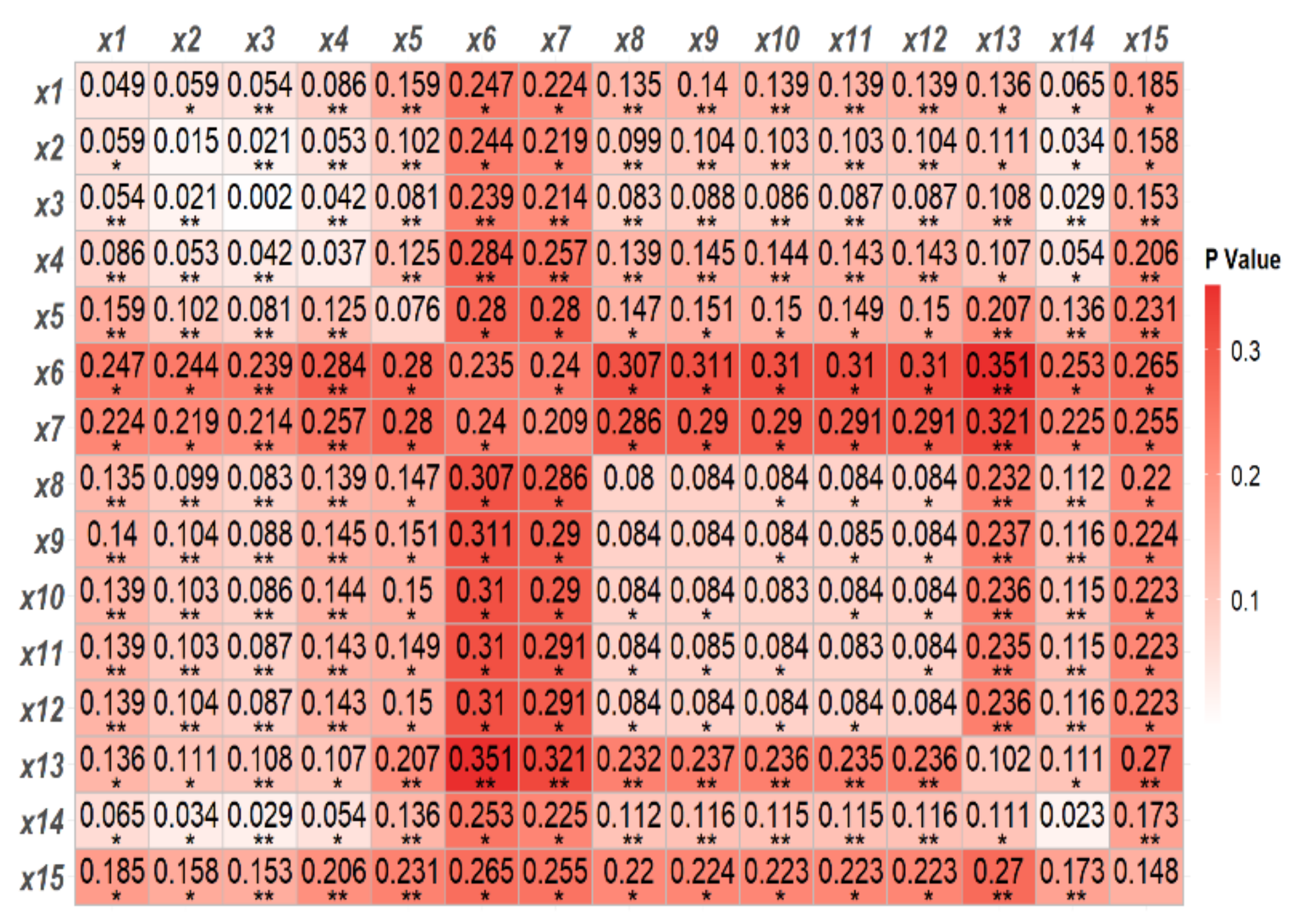
Interaction detector: analyzes the possible causal relationships between different influencing factors, i.e., whether the combined effect of different factors enhances the explanatory power of EV. In the evaluation process, we first calculate the q-values of Y for each of the two factors: q(X1) and q(X2); calculate the q-value of Y when the two layers are tangent: q(X1∩X2); and compare q(X1), q(X2), and q(X1∩X2). The relationship is detailed in the

Table 3. Interaction relationship.

Criterion	Interaction
q(X1∩X2) < Min(q(X1), q X2))	Non-linear weakening
Min(q(X1), q(X2)) < q(X1∩X2) < Max(q(X1), q(X2))	Single-factor non-linear attenuation
q(X1∩X2) > Max(q(X1), q(X2))	Two-factor enhancement
q(X1∩X2) = q(X1) + q(X2)	Independent
q(X1∩X2) > q(X1) + q(X2)	Non-linear enhancement

[64].

3. Results

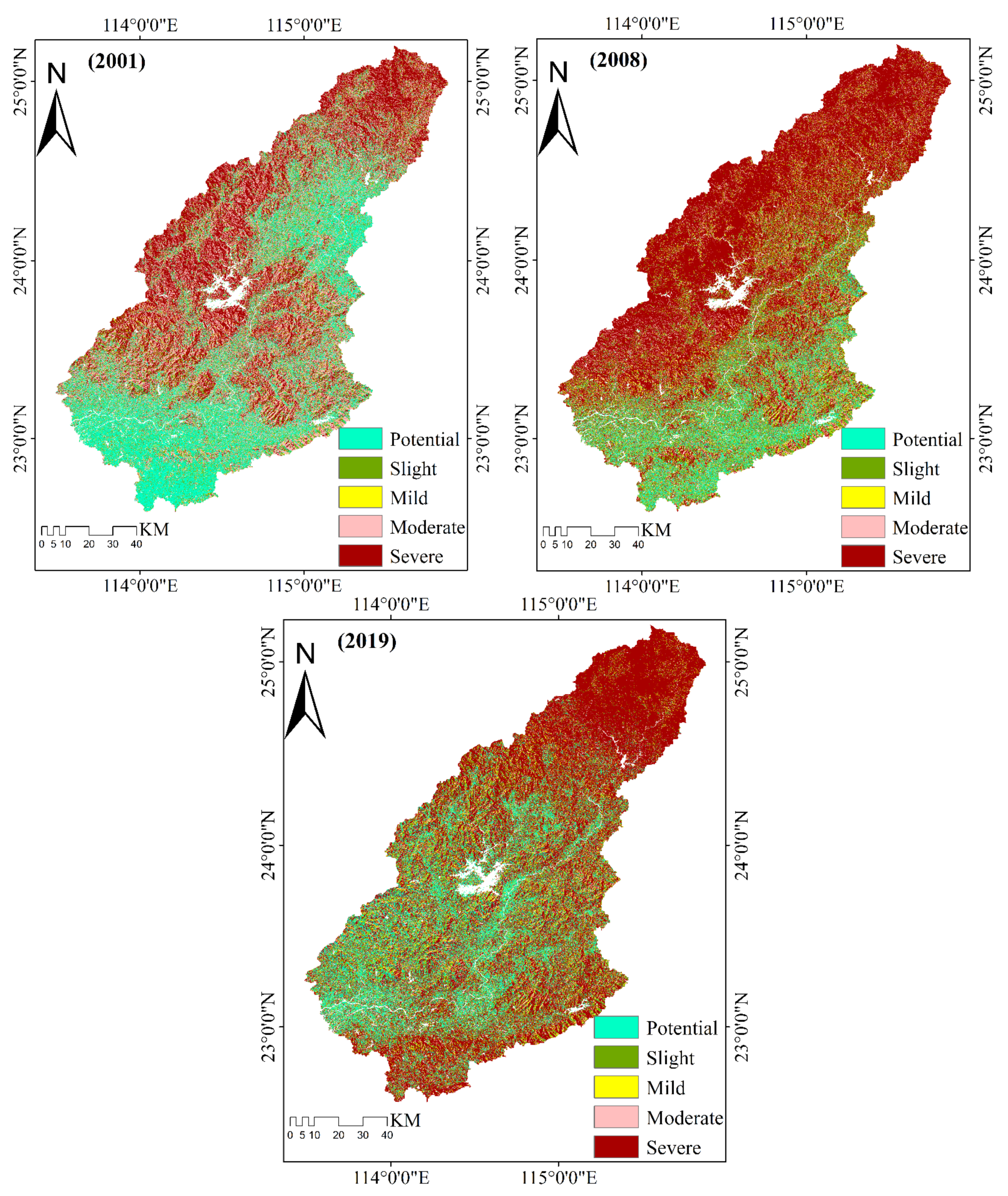
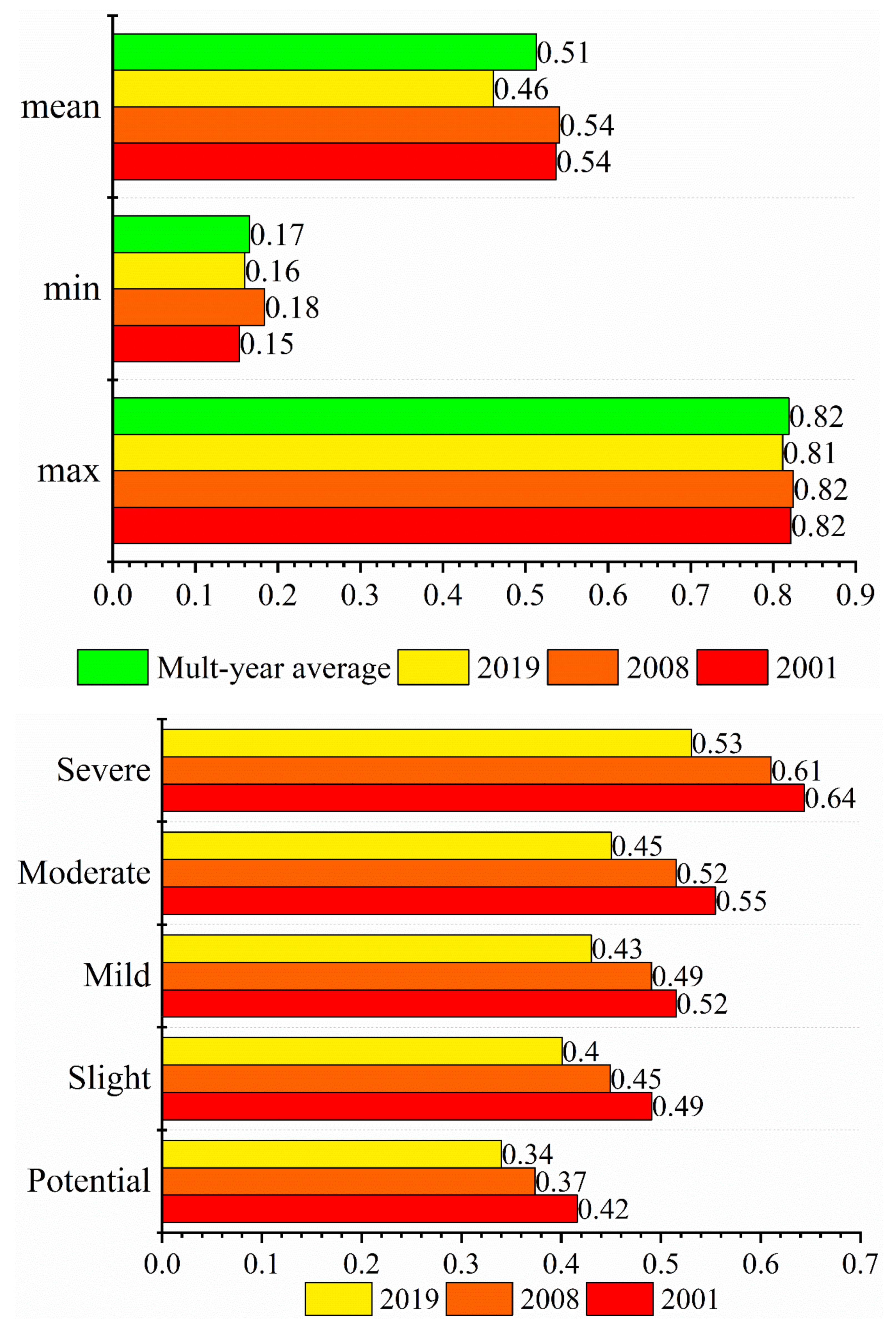
3.1. Temporal Evolution Characteristics of Ecological Vulnerability

On the basis of the establishment of the PSR EV model in the previous section, the spatial distribution of the EV index in the study area was calculated using Equation (6). The grading map (Figure 3) and the percentage of area in EV levels (

Table 4. Statistics on the percentage of area at each EV level in the DRB (2001, 2008, 2019).

Level	Vulnerability Level	2001	2008	2019
		Percentage of the Total Area (%)	Percentage of the Total Area (%)	Percentage of the Total Area (%)
I	Potential	23	8	17
II	Slight	14	17	15
III	Mild	4	7	9
IV	Moderate	29	13	9
V	Severe	30	55	50

) were calculated.

This research reclassified the EV values in 2001, 2008, and 2019 in the DRB, and then obtained three periods of vulnerability level results in this area, which are shown in Figure 4. According to the level results, the research also counted the coverage and area proportion of each classification, which are shown in

Table 5. Statistics of q-values for ecological vulnerability factor detection.

Name of the Factor	2001			2008			2019
	q	q Ranking	p	q	q Ranking	p	q	q Ranking	p
Soil erosion(X4)	0.109	10	0	0.066	10	0	0.037	12	0
Area_mn(X8)	0.057	15	0	0.046	14	0	0.080	9	0
Slope orientation(X3)	0.250	5	0	0.259	2	0	0.002	15	0
Vegetation cover(X13)	0.280	3	0	0.208	4	0	0.102	4	0
Elevation(X1)	0.258	4	0	0.207	5	0	0.049	11	0
Boundary density (ed) (X9)	0.057	14	0	0.049	13	0	0.084	5	0
GDP per capita(X15)	0.132	9	0	0.089	9	0	0.148	3	0
Average annual precipitation(X5)	0.245	6	0	0.145	6	0	0.076	10	0
Population density(X14)	0.172	7	0	0.133	7	0	0.023	13	0
Average annual temperature(X6)	0.284	2	0	0.226	3	0	0.235	1	0
Shannon Diversity Index (SHDI) (X10)	0.059	11	0	0.050	11	0	0.083	8	0
Shannon’s evenness index (SHEI) (X11)	0.058	12	0	0.009	15	0	0.083	7	0
Relative Humidity(X7)	0.325	1	0	0.329	1	0	0.209	2	0
Simpson diversity index (SIDI) (X12)	0.058	13	0	0.050	12	0	0.084	6	0
Slope(X2)	0.144	8	0	0.090	8	0	0.015	14	0

. In 2001, 2008, and 2019, the EV index of the DRB ranged from 0.15 to 0.82, with an annual average of 0.51, as shown in Figure 5. According to the analysis of statistics in

Table 6. Interaction results for selected factors of ecological vulnerability in the DRB.

2001		2008		2019
X3/X7 *	0.564	X3/X7 *	0.570	X13/X6 *	0.351
X3/X6 **	0.535	X13/X7 *	0.505	X13/X7 *	0.321
X3/X13 *	0.528	X3/X6 **	0.476	X9/X6 *	0.311
X13/X7 *	0.517	X3/X13 *	0.471	X6/X12 *	0.311
X3/X1 *	0.506	X3/X1 *	0.464	X6/X11 *	0.310
X3/X5 **	0.502	X4/X7 **	0.442	X6/X10 *	0.310
X13/X6 *	0.481	X13/X6 *	0.434	X8/X6 *	0.307
X13/X5 *	0.454	X3/X5 **	0.402	X7/X12 *	0.291
X4/X7 **	0.447	X15/X7 *	0.394	X11/X7 *	0.291
X3/X14 **	0.426	X3/X14 **	0.394	X9/X7 *	0.291
X3/X2 **	0.405	X10/X7 *	0.394	X10/X7 *	0.290
X4/X6 **	0.403	X7/X12 *	0.394	X8/X7 *	0.287
X1/X7 *	0.397	X9/X7 *	0.393	X4/X6 **	0.284
X5/X7 *	0.396	X8/X7 *	0.388	X5/X6 *	0.280
X1/X6 *	0.393	X13/X5 *	0.379	X5/X7 *	0.280
X15/X7 *	0.388	X5/X7 *	0.379	X13/X6 *	0.270
X6/X7 *	0.385	X1/X7 *	0.368	X15/X6 *	0.265
X3/X15 **	0.383	X6/X7 *	0.367	X4/X7 **	0.257
X13/X15 *	0.382	X15/X6 *	0.354	X15/X7 *	0.255
X10/X7 *	0.380	X3/X15 **	0.354	X14/X6 *	0.253

(* represents a two-factor enhanced interaction, ** represents a non-linear enhanced interaction).

, the proportion of severe (V) level in the DBR was the highest in all three periods, increasing and then decreasing, indicating that EV in the DBR deteriorated and then improved. The proportion of moderate (IV) level was the lowest in all periods. The proportion of mild (III) level decreased year by year. The proportion of slight (II) level increased and then decreased, and the proportion of potential (I) level followed the opposite trend. At the macro level, the overall fragility of the eco-environment in the DRB decreased from north to south.

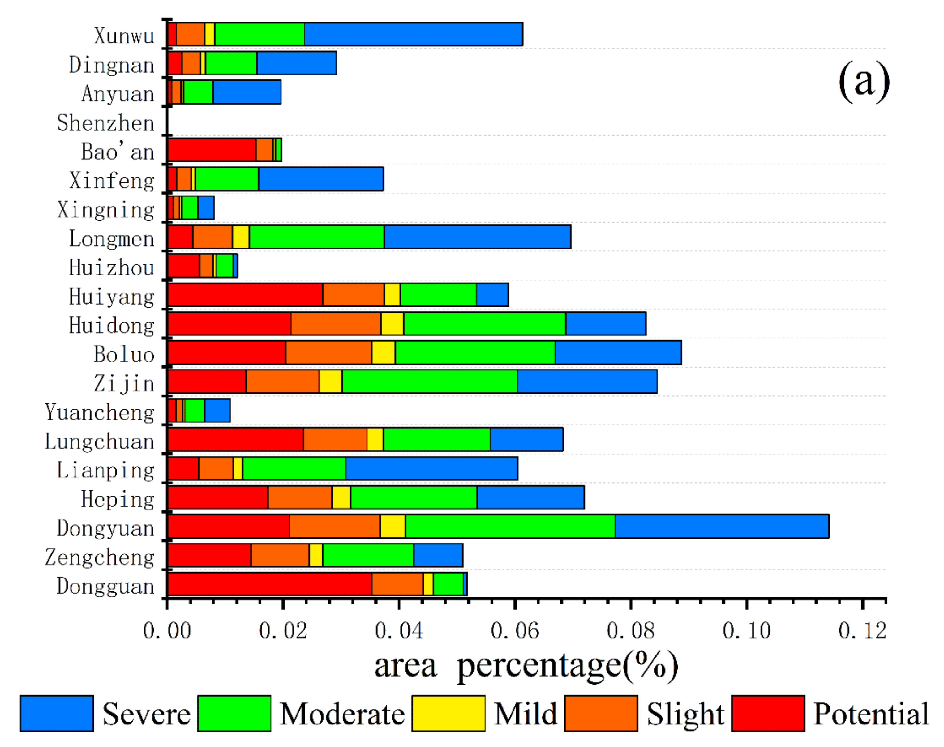
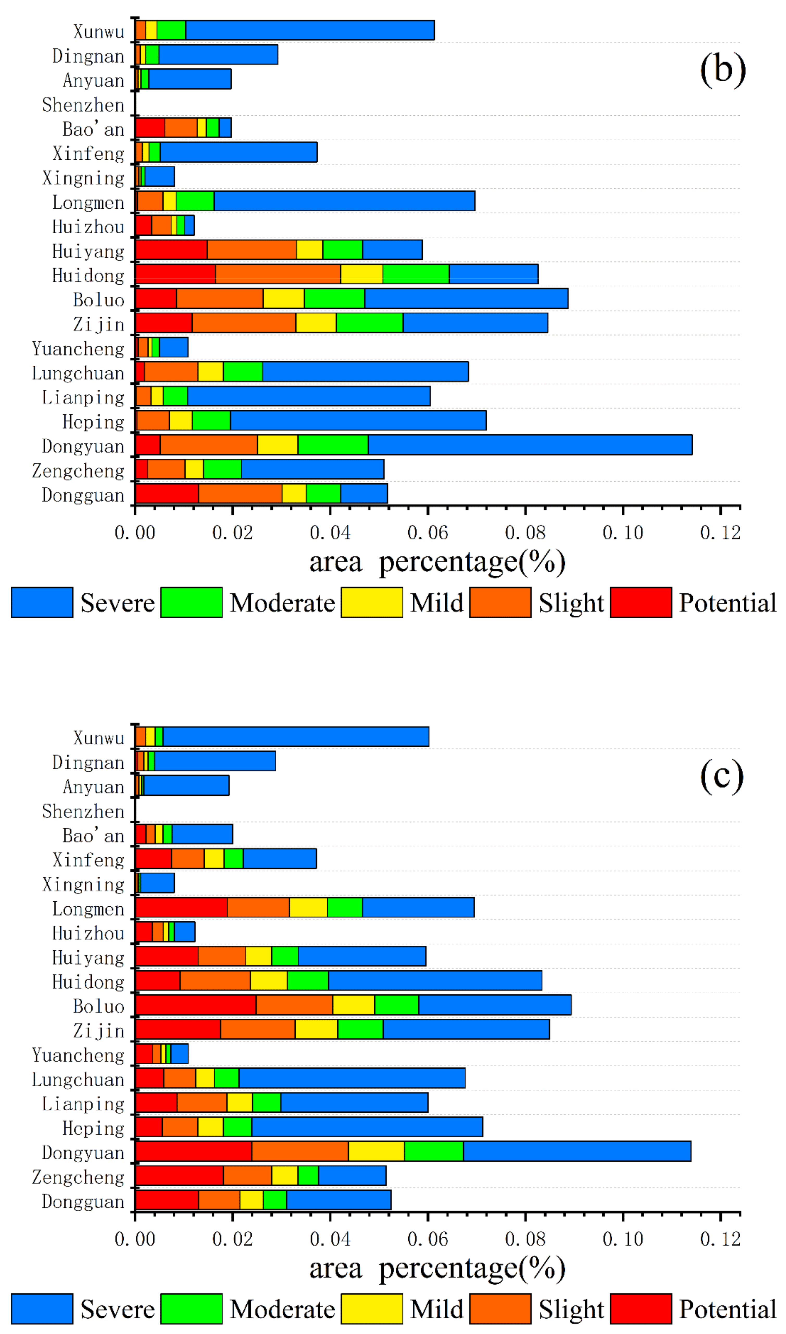
3.2. Change of Ecological Vulnerability Grade Index

We calculated the spatial distribution of the EV change intensity in 2001, 2008, and 2019. Then, we differentiated the vulnerability maps for the three years (2001, 2008, and 2019), and the spatio-temporal changes in EV in the DRB were further analyzed. On the basis of the histogram distribution and related spatio-temporal map changes, the four stages of EV change intensity (CI) were classified as follows: decreasing intensity (CI ≤ −0.20); mildly decreasing (−0.20 < CI ≤ −0.1); stable (−0.1 < CI ≤ 0); mildly increasing (0< CI ≤ 0.1); and intensity increase (CI > 0.1). We used the ArcGIS zonal statistics tool to calculate the average of each factor for each district and county and combined it with Figure 6. The results show that, from 2001 to 2008 (Figure 6A), the DRB was dominated by two intensities, i.e., mild increase and stable, with mild increase occupying more than half and stable mainly distributed in Huidong, Zijin, Huizhou, Yuancheng, Dongyuan, and Boluo. From 2008 to 2019 (Figure 6B), mild decrease was mainly distributed in Zengcheng, Boluo, Longmen, Lianping, Dongyuan, and Yuancheng, etc., and mild increase dominated in Shenzhen, Dongguan, Huiyang, Huizhou, and Huidong in the southern DRB. The quality of the environment has improved over the last 20 years in the DRB, with a trend towards increased EV in a few areas, these being more obvious is the southernmost part of the DRB (Figure 6C).

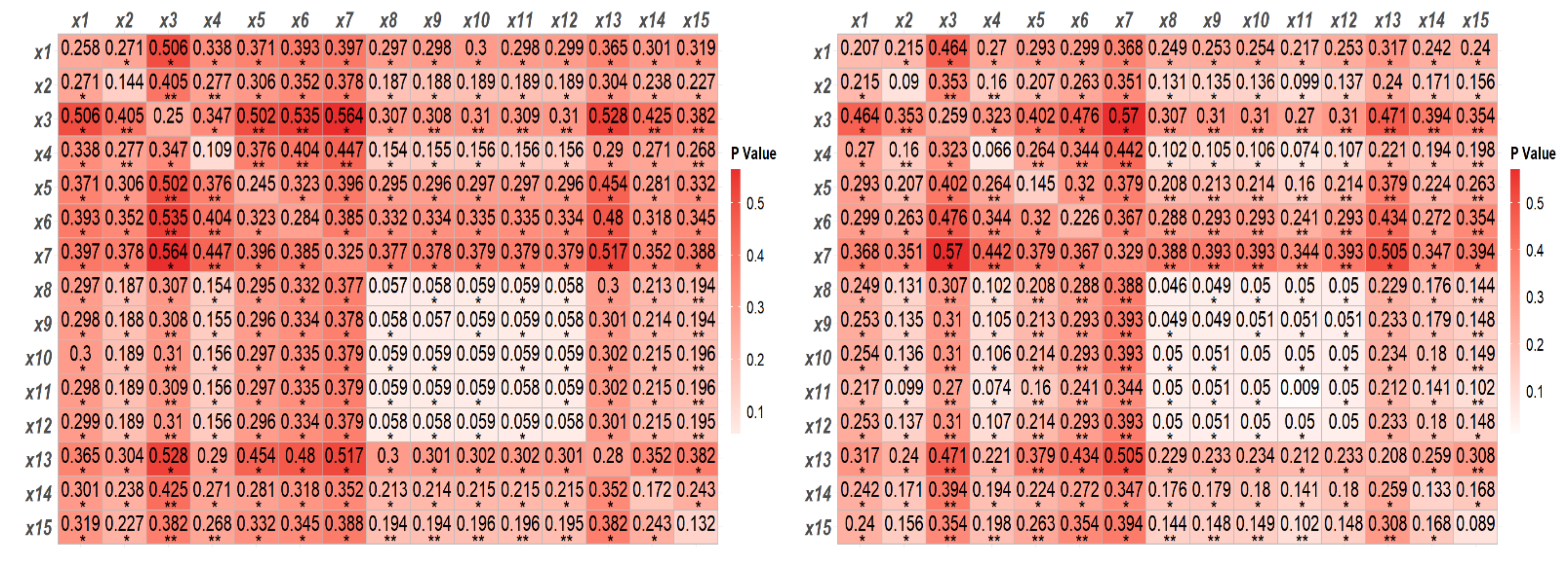
3.3. Analysis of the Drivering Factors of Ecological Vulnerability

We used the ArcGIS 10.2 software to create 30 m × 30 m grid points and extracted 18,249 sample points. We relied on the aforementioned sample points to extract the values of each dependent and independent variable for the quantitative analysis and evaluation of the driving force factors. EV was selected as the dependent variable, and the 15 EV factors were selected as the independent variables. After standardizing them, the factors for each period (2001, 2008, and 2019) were transformed from numerical quantities to typological quantities using the natural breakpoint method at five levels. Finally, we used Geodetector to analyze the impact of each factor on EV. Factor detectors were used to calculate the influence of each factor on EV. As can be seen from Table 5, the p-value of each factor was 0, which indicates that the explanatory power of the three period factors on EV was sufficient. This also proves that the selection of topography, climate, vegetation, landscape, and economic factors to calculate the EV of the DRB was feasible. In general, the influence of the DRB factors on EV was basically stable. From these, the top two q-values were relative humidity and average annual temperature, with mean q-values of 0.288 and 0.248, respectively, indicating that the EV of the DRB was most influenced by relative humidity and average annual temperature. This is mainly due to the fact that relative humidity and average annual temperature are the dominant factors affecting evapotranspiration in most parts of China [65]. The DRB is located in the humid subtropical monsoon climate of southern China, with abundant but unevenly distributed rainfall; the average annual temperature is 20–22 °C, with little average annual temperature variation [66]. Evapotranspiration affects regional climate change and vegetative growth, and thus the EV of the DRB [67].

From 2001 to 2008, the q-values in the 3–6 range were mainly vegetative cover, elevation, and precipitation. They exhibit a decreasing trend, indicating that the influence of these three factors on the EV was gradually weakening. This is mainly because the DRB is located in the humid region of southern China, with undulating terrain and dense vegetation; changes in the ecological environment are largely influenced by vegetative cover, elevation, and precipitation. The q-values in 2019 were mainly for GDP per capita, which is very different from the rankings in 2001 and 2008. As the DRB has undergone a rapid developmental process in recent years, in general, the q-value of GDP per capita exhibits an upward trend, which indicates a gradual rise in the impact of social activities on EV.

Interaction detection was used to assess whether the explanatory power of EV was enhanced when the two factors acted together. Overall (Table 6, Figure 7), the values of the EV factor interactions were greater than the maximum values of the individual factors, thus indicating that the effects of the factors on EV were not independent of each other, but occurred synergistically. As shown in the table, from 2001 to 2008, all the factors were bi-factorially enhanced, except for slope orientation, which was non-linearly enhanced with precipitation, average annual temperature, population density, and GDP per capita. In 2019, soil erosion was non-linearly enhanced with average annual temperature and relative humidity, and each was bi-factorially enhanced. From 2001 to 2019, the DRB interaction detection results were generally more stable, with relative humidity exhibiting the highest interaction with other factors. Moreover, the interaction of the relative humidity with the other factors was much higher than the number of interactions between two of the other factors that occurred. The interaction between topography, climate, vegetation, landscape, and economic factors was stronger than the interaction within each element, and the interaction between natural and social factors was stronger than the interaction within each factor, indicating that the EV of the DRB was the result of the combined effect of all factors.

4. Conclusions and Discussions

4.1. Discussions

We took the DRB as the study area and constructed factor models to analyze the current situation through regional ecological problems. On the basis of the statistical data, such as multi-temporal remote sensing data and multi-year meteorological station data, this study used socio-economic statistics to characterize anthropogenic disturbance factors and analyze the characteristics of EV. As a result of the high level of human activity in the DRB, its ecosystem is under a certain amount of development pressure. In this study, we also conducted a scientific analysis of the manifestation factors of EV from 2001–2019 in terms of ecological pressure, ecological sensitivity, and ecological resilience, and screened out various practical and typical integrated factors. In addition, vegetation inversion, soil erosion factors, landscape pattern factors, and spatial interpolation were constructed as evaluation factors based on three time periods from 2001–2019. Finally, the DRB EV evaluation index system was established.

PCA generates principal components that are independent of each other after the transformation of the original factors, which can reduce the workload of factor selection. The weights of the principal components, i.e., the contribution rate, contain the proportion of the information from the original data to the total information, and thus, this is considered an objective and reasonable assessment. Therefore, we used PCA to evaluate the EV of the DRB. In addition, using the interpolation method, the overall trend state index, and the comprehensive EV index, with the method of dynamically determining the EV rating of NPP data used by Guo Bing [10], we finally analyzed the change in the EV rating in the area, the overall EV trend, and the quality state of each district in the DRB for three periods of vulnerability from 2001 to 2019.

The factors influencing the EV in the DRB were analyzed with the help of the Geodetector software developed by Wang Jinsong [64] et al. in order to obtain objective and scientific results. This can also be confirmed by the research results of Guo Zeqing [56] et al. and Liu Jiaru [68] et al. In this study, Geodetector was used to analyze the magnitude of interactions between various factors in the EV model for each period and the anthropogenic drivers of EV in the DRB.

On the basis of a PSR model with 15 evaluation factors, we analyzed the spatial distribution of EV in the DRB over three periods and, using a geographic probe, carried out a quantitative statistical analysis of the factors driving EV. The results show that EV is decreasing from 2001 to 2019, with a stronger explanatory power for relative humidity, mean annual temperature, and vegetation cover as the main driving factors of EV in the DRB in the 3 years. In 2019, the explanatory power of GDP per capita increases, showing that human activities further influence EV in the DRB. The relative humidity and mean annual temperature did not change much [66]. Moreover, the woodland cover of the DRB increased from 2001 to 2019 (Figure 8), showing that woodland ecosystems are the most functional and structurally complex natural ecosystems of terrestrial ecosystems. Thus, they have a decisive influence on the terrestrial ecosystem environment and play an important role in safeguarding the ecosystem [69,70]. They are not only capable of providing production and living resources for humans, they also have a variety of ecological service functions, such as water containment, carbon sequestration, oxygen release, and maintaining regional ecological balance, which are important for maintaining the environment and promoting a sustainable urban development [71]. This coincides with a consistent decrease in EV. Furthermore, in the interaction detection results, the study found that the interaction between two driving factors had a greater impact on EV in the DRB as compared to a single driving factor (Table 5, Table 6). In both driver indicators, the slope orientation (X3)/relative humidity (X7), slope orientation (X3)/average annual temperature (X6), and slope orientation (X3)/vegetation cover (X13) interactions had the strongest impact on EV in the DBR, in 2001; In 2008, the strongest interaction factors were slope orientation (X3)/relative humidity (X7), vegetation cover (X13)/relative humidity (X7), and slope orientation (X3)/average annual temperature (X6). The interaction factors of vegetation cover (X13)/average annual temperature (X6), vegetation cover (X13)/relative humidity (X7), and (X9)/average annual temperature (X6) were strongest in 2019 (Table 6). Ecosystems are complex systems where some factors interact with each other. For example, the transpiration of the vegetation increases relative humidity, and changes in vegetation cover affect relative humidity [59]. Jiang [72] showed that vegetation has the ability to change the climate of an ecosystem. Moreover, we found that vegetation cover had a strong EV explanatory power in all three years (Table 5). Limpid waters and lush mountains are invaluable assets. Therefore, we believe that planned afforestation is a worthwhile project that may influence (improve) EV.

However, the evolution of the spatio-temporal patterns of EV in the DRB from 2001 to 2019 was also influenced by many other uncontrollable natural factors and multi-level human socio-economic factors. Importantly, future studies need to cover a wide range of scientific fields and thus analyze the evolution of EV in the DRB in all its complexity. To this end, more factors must be considered in future studies.

4.2. Conclusions

The DRB, which is an ecologically fragile area in South China, has an important strategic position in terms of resources, environment, and ecology. In view of the unique geographical characteristics and the limitations of relevant studies, we selected 15 well-structured and statistically significant factors, such as topography, climate, landscape, and socio-economy, to analyze the EV status of the DRB. Furthermore, we analyzed its spatio-temporal changes based on the PCA analysis, and detected the driving factors using geographic probes. The following conclusions were reached:

(1)

The PCA method can objectively and reasonably calculate the changes in each factor in the process of assigning weights to vulnerability factors in multi-temporal studies. The method can better reflect the change process of each factor in the EV system, and has good applicability in the southern red soil hilly ecosystem of China.

(2)

NPP data can be associated with the assessment of the health of land surface ecosystems, and the EV level thresholds in different periods can be obtained with the aid of NPP data calculation, which is important for the analysis of EV in different years.

(3)

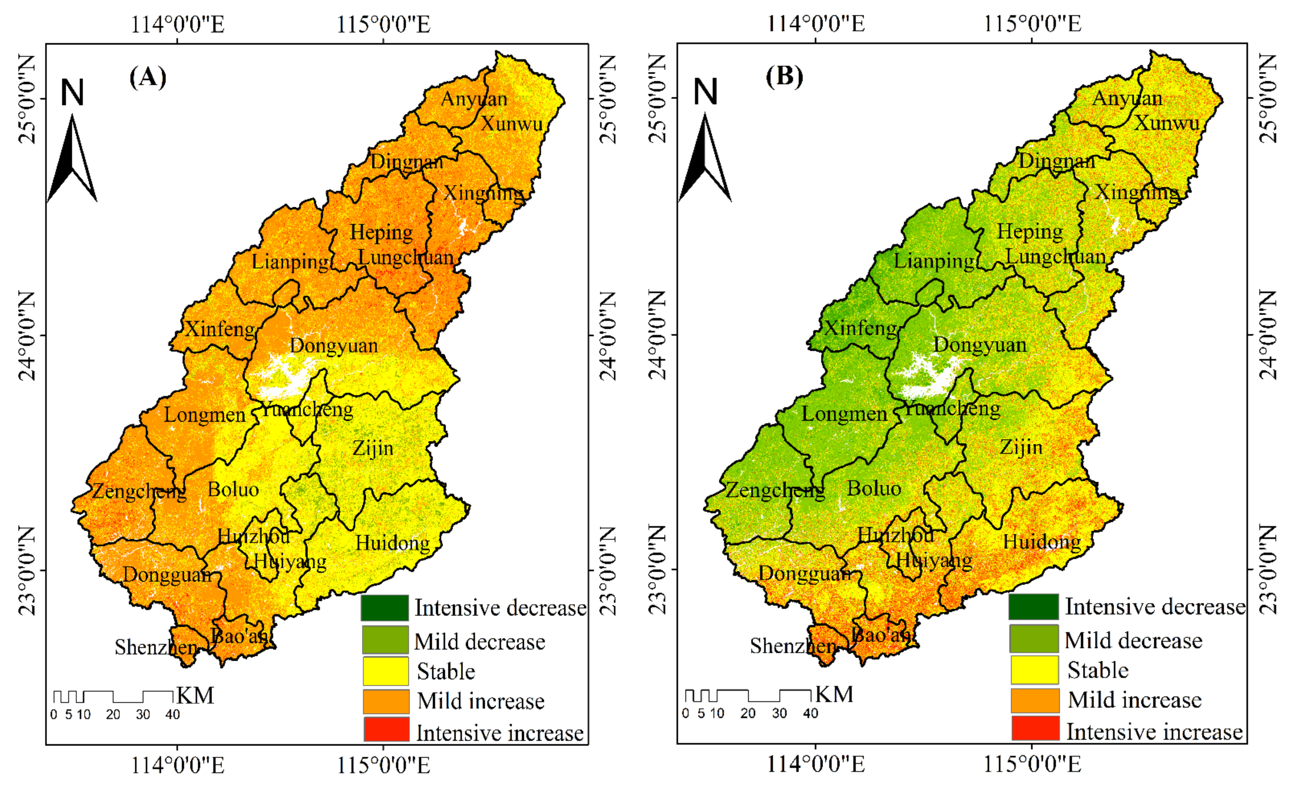
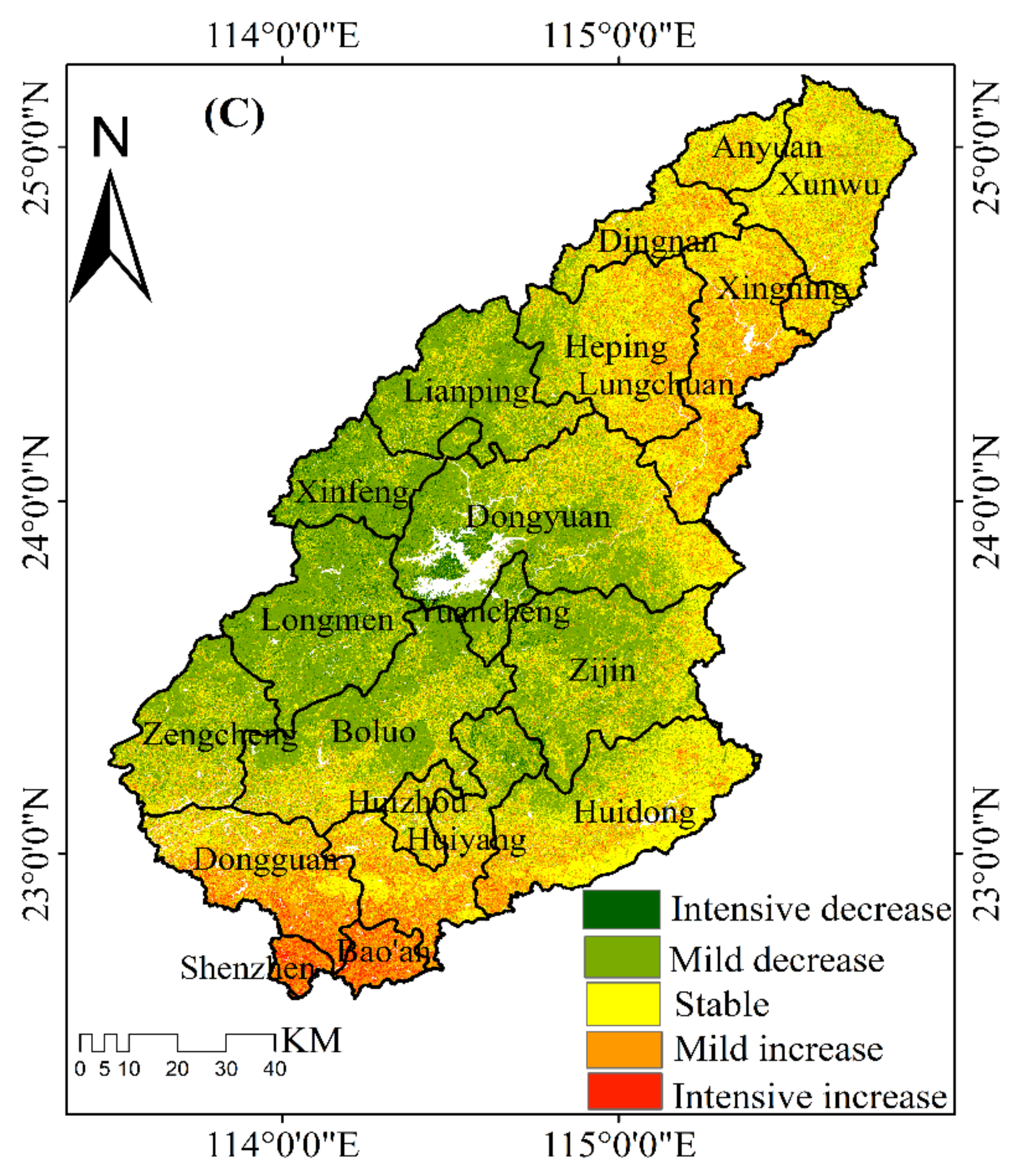
Over the past 20 years, the overall EV intensity in the DRB can be characterized by a mild decrease, while the upstream and downstream EV intensity in the DRB can be characterized by a mild increase. The midstream exhibited a mild decrease. From 2001 to 2019, the mean EV value gradually decreased. From 2001 to 2008, The area of EV intensity for mild increase is much larger than stable. From 2008 to 2019, EV intensity is more widely distributed in areas of mild decrease than mild increase.

(4)

During 2001–2019, the spatio-temporal pattern of EV in the DRB was significantly affected by the relative humidity, average annual temperature, and vegetation cover.

References

1. Depietri, Y. The social–ecological dimension of vulnerability and risk to natural hazards. Sustain. Sci. 2020, 15, 587–604. [Google Scholar] [CrossRef]
2. Lv, X.; Xiao, W.; Zhao, Y.; Zhang, W.; Li, S.; Sun, H. Drivers of spatio-temporal ecological vulnerability in an arid, coal mining region in Western China. Ecol. Indic. 2019, 106, 105475. [Google Scholar] [CrossRef]
3. Bouwer, L.M. Have disaster losses increased due to anthropogenic climate change? Bull. Am. Meteorol. Soc. 2011, 92, 39–46. [Google Scholar] [CrossRef] [Green Version]
4. Gu, D.; Gerland, P.; Pelletier, F.; Cohen, B. Risks of exposure and vulnerability to natural disasters at the city level: A global overview. United Nations Tech. Pap. 2015, 2, 1–40. [Google Scholar]
5. Pachauri, R.K.; Allen, M.R.; Barros, V.R.; Broome, J.; Cramer, W.; Christ, R.; Church, J.A.; Clarke, L.; Dahe, Q.; Dasgupta, P.; et al. Climate Change 2014: Synthesis Report. In Contribution of Working Groups I, II and III to the Fifth Assessment Report of the Intergovernmental Panel on Climate Change; IPCC: Geneva, Switzerland, 2014. [Google Scholar]
6. Niu, W.Y. Improvement of ablers model with regard to searching of geographical space. Chin. Sci. Bull. 1989, 34, 155–157. [Google Scholar]
7. Clements, F.E. Research Methods in Ecology; University Publishing Company: Lincoln, Nebraska, 1905. [Google Scholar]
8. Liao, X.; Li, W.; Hou, J. Application of GIS based ecological vulnerability evaluation in environmental impact assessment of master plan of coal mining area. Procedia Environ. Sci. 2013, 18, 271–276. [Google Scholar] [CrossRef] [Green Version]
9. Nelson, R.; Kokic, P.; Crimp, S.; Martin, P.; Meinke, H.; Howden, S.M.; Voil, P.D.; Nidumolu, U. The vulnerability of Australian rural communities to climate variability and change: Part II—Integrating impacts with adaptive capacity. Environ. Sci. Policy 2010, 13, 18–27. [Google Scholar] [CrossRef]
10. Guo, B.; Zang, W.; Luo, W. Spatial-temporal shifts of ecological vulnerability of Karst Mountain ecosystem-impacts of global change and anthropogenic interference. Sci. Total Environ. 2020, 741, 140256. [Google Scholar] [CrossRef]
11. Keyes, A.A.; McLaughlin, J.P.; Barner, A.K.; Dee, L.E. An ecological network approach to predict ecosystem service vulnerability to species losses. Nat. Commun. 2021, 12, 1586. [Google Scholar] [CrossRef]
12. Chang, H.; Pallathadka, A.; Sauer, J.; Grimm, N.B.; Herreros-Cantis, P. Assessment of urban flood vulnerability using the social-ecological-technological systems framework in six US cities. Sustain. Cities Soc. 2021, 68, 102786. [Google Scholar] [CrossRef]
13. Boori, M.S.; Choudhary, K.; Paringer, R.; Kupriyanov, A. Spatiotemporal ecological vulnerability analysis with statistical correlation based on satellite remote sensing in Samara, Russia. J. Environ. Manag. 2021, 285, 112138. [Google Scholar] [CrossRef]
14. Mafi-Gholami, D.; Pirasteh, S.; Ellison, J.C.; Jaafari, A. Fuzzy-based vulnerability assessment of coupled social-ecological systems to multiple environmental hazards and climate change. J. Environ. Manag. 2021, 299, 113573. [Google Scholar] [CrossRef]
15. Turner, B.L.; Kasperson, R.E.; Matson, P.A.; McCarthy, J.J.; Corell, R.W.; Christensen, L.; Eckley, N.; Kasperson, J.X.; Luers, A.; Martello, M.L.; et al. A framework for vulnerability analysis in sustainability science. Proc. Natl. Acad. Sci. USA 2003, 100, 8074–8079. [Google Scholar] [CrossRef] [Green Version]
16. Wang, B.; Ding, M.; Guan, Q.; Ai, J. Gridded assessment of eco-environmental vulnerability in Nanchang city. Acta Ecol. Sin. 2019, 39, 5460–5472. [Google Scholar]
17. Yang, Y.; Song, G. Human disturbance changes based on spatiotemporal heterogeneity of regional ecological vulnerability: A case study of Qiqihaer city, northwestern Songnen Plain, China. J. Clean. Prod. 2021, 291, 125262. [Google Scholar] [CrossRef]
18. Xia, M.; Jia, K.; Zhao, W.; Liu, S. Spatio-temporal changes of ecological vulnerability across the Qinghai-Tibetan Plateau. Ecol. Indic. 2021, 123, 107274. [Google Scholar] [CrossRef]
19. Li, Q.; Shi, X.; Wu, Q. Effects of protection and restoration on reducing ecological vulnerability. Sci. Total Environ. 2021, 761, 143180. [Google Scholar] [CrossRef]
20. Tang, Q.; Wang, J.; Jing, Z. Tempo-spatial changes of ecological vulnerability in resource-based urban based on genetic projection pursuit model. Ecol. Indic. 2021, 121, 107059. [Google Scholar] [CrossRef]
21. Jin, Y.; Li, A.; Bian, J.; Nan, X.; Lei, G.; Muhammand, K. Spatiotemporal analysis of ecological vulnerability along Bangladesh-China-India-Myanmar economic corridor through a grid level prototype model. Ecol. Indic. 2021, 120, 106933. [Google Scholar] [CrossRef]
22. Dai, X.; Gao, Y.; He, X.; Liu, T.; Jiang, B.; Shao, H.; Yao, Y. Spatial-temporal pattern evolution and driving force analysis of ecological environment vulnerability in Panzhihua City. Environ. Sci. Pollut. Res. 2021, 28, 7151–7166. [Google Scholar] [CrossRef]
23. Huang, M.; Zhong, Y.; Feng, S.; Zhang, J. Spatial and temporal characteristics and drivers of landscape ecological vulnerability in the Chaohu Lake Basin since 1970s. Lake Sci. 2020, 32, 977–988. [Google Scholar]
24. Hu, X.; Ma, C.; Huang, P.; Guo, X. Ecological vulnerability assessment based on AHP-PSR method and analysis of its single parameter sensitivity and spatial autocorrelation for ecological protection–A case of Weifang City, China. Ecol. Indic. 2021, 125, 107464. [Google Scholar] [CrossRef]
25. Kang, H.; Tao, W.; Chang, Y.; Zhang, Y.; Li, X.; Chen, P. A feasible method for the division of ecological vulnerability and its driving forces in Southern Shaanxi. J. Clean. Prod. 2018, 205, 619–628. [Google Scholar] [CrossRef]
26. Xie, Z.; Li, X.; Chi, Y.; Jiang, D.; Chen, S. Ecosystem service value decreases more rapidly under the dual pressures of land use change and ecological vulnerability: A case study in Zhujiajian Island. Ocean Coast. Manag. 2021, 201, 105493. [Google Scholar] [CrossRef]
27. Shi, H.; Lu, J.; Zheng, W.; Sun, J.; Ding, D. Evaluation system of coastal wetland ecological vulnerability under the synergetic influence of land and sea: A case study in the Yellow River Delta, China. Mar. Pollut. Bull. 2020, 161, 111735. [Google Scholar] [CrossRef]
28. Liu, M.; Liu, X.; Wu, L.; Tang, Y.; Li, Y.; Zhang, Y.; Ye, L.; Zhang, B. Establishing forest resilience indicators in the hilly red soil region of southern China from vegetation greenness and landscape metrics using dense Landsat time series. Ecol. Indic. 2021, 121, 106985. [Google Scholar] [CrossRef]
29. Xue, L.; Jing, W.; Zhang, L.; Wei, G.; Zhou, B. Spatiotemporal analysis of ecological vulnerability and management in the Tarim River Basin, China. Sci. Total Environ. 2019, 649, 876–888. [Google Scholar] [CrossRef]
30. Wu, C.; Liu, G.; Huang, C.; Liu, Q.; Guan, X. Ecological vulnerability assessment based on fuzzy analytical method and analytic hierarchy process in Yellow River Delta. Int. J. Environ. Res. Public Health 2018, 15, 855. [Google Scholar] [CrossRef] [PubMed] [Green Version]
31. Nguyen, K.A.; Liou, Y.A. Global mapping of eco-environmental vulnerability from human and nature disturbances. Sci. Total Environ. 2019, 664, 995–1004. [Google Scholar] [CrossRef] [PubMed]
32. Wang, Y. Effects of Different Vegetation Restoration Patterns on Soil Reactive Organic Carbon in the Antaibao Mining Area; China University of Geosciences: Beijing, China, 2015. [Google Scholar]
33. He, Y.; Guo, H.; Tan, Q.; Pan, W.; Chen, S. Identification of significant water problems in the Dongjiang River Basin of Guangdong Province. Water Resour. Conserv. 2021, 37, 16–21. [Google Scholar]
34. Lv, L.; Gao, X.Q.; Liu, Q.; Jiang, Y. Effects of landscape patterns on nitrogen and phosphorus export in the Dongjiang River Basin. J. Ecol. 2021, 41, 1758–1765. [Google Scholar]
35. Lv, L.T.; Zhang, J.; Peng, Q.Z.; Ren, F.P.; Jiang, Y. Analysis of landscape pattern evolution and prediction of changes in the Dongjiang River Basin. J. Ecol. 2019, 39, 6850–6859. [Google Scholar]
36. Jiang, Q.; Zhou, P.; Liao, C.; Liu, Y.; Liu, F. Spatial pattern of soil erodibility factor (K) as affected by ecological restoration in a typical degraded watershed of central China. Sci. Total Environ. 2020, 749, 141609. [Google Scholar] [CrossRef]
37. Amundson, R.; Berhe, A.A.; Hopmans, J.W.; Olson, C.; Sztein, A.E.; Sparks, D.L. Soil and human security in the 21st century. Science 2015, 348. [Google Scholar] [CrossRef] [Green Version]
38. Wang, B.; Zheng, F.; Römkens, M.J.M.; Darboux, F. Soil erodibility for water erosion: A perspective and Chinese experiences. Geomorphology 2013, 187, 1–10. [Google Scholar] [CrossRef]
39. Williams, J.R. The erosion-productivity impact calculator (EPIC) model: A case history. Philosophical Transactions of the Royal Society of London. Ser. B Biol. Sci. 1990, 329, 421–428. [Google Scholar]
40. Diao, C.; Wang, L. Landsat time series-based multiyear spectral angle clustering (MSAC) model to monitor the inter-annual leaf senescence of exotic saltcedar. Remote Sens. Environ. 2018, 209, 581–593. [Google Scholar] [CrossRef]
41. Mao, X.P.; Diao, J.J.; Fan, J.H.; Lui, Y.Y.; Xu, N.G.; Wang, Z.; Li, M.S. Analysis and prediction of landscape dynamics in the forest-grass mosaic zone of the Daxingan Mountains, Inner Mongolia. J. Ecol. 2021, 1–12. [Google Scholar]
42. Xue, S.-S.; Gao, F.; He, B.; Yan, Z.-G. Analysis of landscape patterns and driving forces in the Wulungu River basin from 1989–2017. Ecol. Sci. 2021, 40, 33–41. [Google Scholar]
43. Cui, T.-X.; Gong, Z.-N.; Zhao, W.-J.; Zhao, Y.-L.; Lin, C. Extraction method of wetland vegetation cover under different end element models: An example from the Beijing Wild Duck Lake Wetland Nature Reserve. J. Ecol. 2013, 33, 1160–1171. [Google Scholar]
44. National Bureau of Statistics. Statistical Yearbook of Jiangxi Province; China Statistics Press: Beijing, China, 2002 2009 2020. [Google Scholar]
45. National Bureau of Statistics. Statistical Yearbook of Guangdong Province; China Statistics Press: Beijing, China, 2002 2009 2020. [Google Scholar]
46. Johnson, R.A.; Wichern, D.W. Practical Multivariate Statistical Analysis; Tsinghua University Press: Beijing, China, 2001. [Google Scholar]
47. Zou, T.; Yoshino, K. Environmental vulnerability evaluation using a spatial principal components approach in the Daxing’anling region, China. Ecol. Indic. 2017, 78, 405–415. [Google Scholar] [CrossRef]
48. Siegel, K.J.; Cabral, R.B.; McHenry, J.; Ojea, E.; Owashi, B.; Lester, S.l. Sovereign states in the Caribbean have lower social-ecological vulnerability to coral bleaching than overseas territories. Proc. R. Soc. B 2019, 286, 20182365. [Google Scholar] [CrossRef] [Green Version]
49. Guo, B.; Fan, Y.; Yang, F.; Jiang, L.; Yang, W.; Chen, S.; Gong, R.; Liang, T. Quantitative assessment model of ecological vulnerability of the Silk Road Economic Belt, China, utilizing remote sensing based on the partition-integration concept. Geomat. Nat. Hazards Risk. 2019, 10, 1346–1366. [Google Scholar] [CrossRef] [Green Version]
50. Zhou, S.; Tian, Y.; Liu, L. Adaptability of agricultural ecosystems in the hilly areas in Southern China a case study in Hengyang Basin. Adaptability of Agricultural Ecosystems in the Hilly Areas in Southern China: A Case Study in Hengyang Basin. Acta Ecol. Sin. 2015, 35, 1991–2002. [Google Scholar]
51. Dai, E.; Li, S.; Wu, Z.; Yan, H.; Zhao, D. Spatial pattern of net primary productivity and its relationship with climatic factors in Hilly Red Soil Region of southern China: A case study in Taihe county, Jiangxi province. Geogr. Res. 2015, 34, 1222–1234. [Google Scholar]
52. Yao, X.; Yu, K.; Liu, J.; Yang, S.; He, P.; Deng, Y.; Yu, X.; Chen, Z. Spatial and temporal changes of the ecological vulnerability in a serious soil erosion area, Southern China. Chin. J. Appl. Ecol. 2016, 27, 735–745. [Google Scholar]
53. Chen, Z.; Yao, X.; Yu, K.; Liu, J. Evolutionary Relation between Ecological Vulnerability and Soil Erosion in the Typical Reddish Soil Region of Southern China. J. Southwest For. Univ. (Nat. Sci.) 2017, 37, 82–90. [Google Scholar]
54. Tian, Y.; Liu, P.; Zheng, W. Vulnerability assessment and analysis of hilly area in Southern China: A case study in the Hengyang Basin. Geogr. Res. 2005, 24, 843–852. [Google Scholar]
55. Fan, S.; Guo, Y.; Qiu, L.; Jiang, C.; Huang, Y. Analyzing the effects of land cover change on urban ecological vulnerability in the central districts of Fuzhou city. J. Fujian Norm. Univ. (Nat. Sci. Ed.) 2018, 34, 92–98. [Google Scholar]
56. Guo, Z.C.; Wei, W.; Pang, S.F.; Zhen, Y.; Zhou, J.; Xie, B. Spatio-temporal evolution and motivation analysis of ecological vulnerability in arid inland river basin based on SPCA and remote sensing index: A case study on the Shiyang River Basin. Acta Ecol. Sin. 2019, 39, 2558–2572. [Google Scholar]
57. Yao, K.; Zhou, B.; Li, X.; He, L.; Li, Y. Evaluation of Ecological Environment Vulnerability in the Upper-Middle Reaches of Dadu River Basin Based on AHP-PCA Entropy Weight Model. Res. Soil Water Conserv. 2019, 26, 265–271. [Google Scholar]
58. Xie, Y.; Tu, X.; Wu, H.; Zhou, W.; Huang, B. Evolution of drought levels and impacts of main factors in the Dongjiang River basin. J. Nat. Disasters 2020, 29, 69–82. [Google Scholar]
59. Shi, X.; Wu, M.; Zhang, N. Characteristics of water use efficiency of typical terrestrial ecosystems in China and its response. Trans. Chin. Soc. Agric. Eng. 2020, 36, 152–159. [Google Scholar]
60. Abd El-Hamid, H.T.; Caiyong, W.; Hafiz, M.A.; Mustafa, E.K. Effects of land use/land cover and climatic change on the ecosystem of North Ningxia, China. Arab. J. Geosci. 2020, 13, 1099. [Google Scholar] [CrossRef]
61. Chen, J.; Luo, M.; Ma, R.; Zhou, H.; Zou, S.; Gan, Y. Nitrate distribution under the influence of seasonal hydrodynamic changes and human activities in Huixian karst wetland, South China. J. Contam. Hydrol. 2020, 234, 103700. [Google Scholar] [CrossRef]
62. Guo, B.; Kong, W.; Jiang, L.; Fan, Y. Analysis of spatial and temporal changes and its driving mechanism of ecological vulnerability of alpine ecosystem in Qinghai Tibet Plateau. Ecol. Sci. 2018, 37, 96–106. [Google Scholar]
63. Jiang, Y.; Li, R.; Shi, Y.; Guo, L. Natural and Political Determinants of Ecological Vulnerability in the Qinghai–Tibet Plateau: A Case Study of Shannan, China. ISPRS Int. J. Geo-Inf. 2021, 10, 327. [Google Scholar] [CrossRef]
64. Wang, J.; Xu, C. Geodetector:principle and prospective. Acta Geogr. Sin. 2017, 72, 116–134. [Google Scholar]
65. Zhou, B.; Li, F.; Xiao, H.; Hu, A.; Yan, L. Characteristics and climate explanation of spatial distribution and temporal variation of potential evapotranspiration in Headwaters of the Three Rivers. J. Nat. Resour. 2014, 29, 2068–2077. [Google Scholar]
66. Lin, K.; He, Y.; Lei, X.; Chen, X. Climate change and its impact on runoff during 1956–2009 in Dongjiang basin. Ecol. Environ. Sci. 2011, 20, 1783–1787. [Google Scholar]
67. Liang, S.; Bai, R.; Chen, X.; Chen, J.; Fan, W.; He, T.; Jia, K.; Jiang, B.; Jiang, L.; Jiao, Z.; et al. Review of China’s land surface quantitative remote sensing development in 2019. J. Remote Sens. 2020, 24, 618–671. [Google Scholar]
68. Liu, J.; Zhao, J.; Shen, S.; Zhao, Y. Ecological vulnerability assessment of Qilian Mountains region based on SRP conceptual model. Arid Land Geogr. 2020, 43, 1573–1582. [Google Scholar]
69. Canadell, J.G.; Raupach, M.R. Managing forests for climate change mitigation. Science 2008, 320, 1456–1457. [Google Scholar] [CrossRef] [Green Version]
70. Gibson, L.; Lee, T.M.; Koh, L.P.; Brook, B.W.; Gardner, T.A.; Barlow, J.; Peres, C.A.; Bradshaw, C.J.; Laurance, W.F.; Lovejoy, T.E.; et al. Primary forests are irreplaceable for sustaining tropical biodiversity. Nature 2011, 478, 378–381. [Google Scholar] [CrossRef]
71. Taye, F.A.; Folkersen, M.V.; Fleming, C.M.; Buckwell, A.; Mackey, B.; Diwakar, K.C.; Le, D.; Hasan, S.; Saint Ange, C. The economic values of global forest ecosystem services: A meta-analysis. Ecol. Econ. 2021, 189, 107145. [Google Scholar] [CrossRef]
72. Jiang, P.; Ding, W.; Yuan, Y.; Ye, W.; Mu, Y. Interannual variability of vegetation sensitivity to climate in China. J. Environ. Manag. 2022, 301, 113768. [Google Scholar] [CrossRef]
Figure 1. Stepwise procedure for spatio-temporal EVI modeling.
Remotesensing 13 04636 g001
Figure 2. Study area. (a) Location of the study area in China; (b) The extent of the DRB; (c) The geographical location of meteorological stations. (The meteorological stations marked in bold are located within the DBR, and the meteorological stations not marked in bold are located outside the DBR).
Remotesensing 13 04636 g002
Figure 3. Distribution of EV levels in the DRB, 2001–2019.
Remotesensing 13 04636 g003
Figure 4. Scale map of vulnerability areas at different levels (a) 2001; (b) 2008; (c) 2019.
Remotesensing 13 04636 g004aRemotesensing 13 04636 g004b
Figure 5. Histogram of minimum, maximum, and mean values based on EV in DRB.
Remotesensing 13 04636 g005
Figure 6. Dynamic changes in EV in DRB. (A) 2008–2001; (B) 2019–2008; (C) 2019–2001.
Remotesensing 13 04636 g006aRemotesensing 13 04636 g006b
Figure 7. The explanatory power of interaction between factors in 2001, 2008, 2019. (* represents a two-factor enhanced interaction, ** represents a non-linear enhanced interaction, p value represents the interaction detection value of the two factors).
Remotesensing 13 04636 g007aRemotesensing 13 04636 g007b
Figure 8. Land use map of DRB (2001, 2008, 2019).
Remotesensing 13 04636 g008aRemotesensing 13 04636 g008b